Int. J. Electrochem. Sci., 4(2009) 1116 - 1127
International Journal of
ELECTROCHEMICAL
SCIENCE
www.electrochemsci.org
Reaction/Diffusion at Electrode/Solution Interfaces: The EC
2Reaction
Michael E G Lyons *
Physical and Materials Electrochemistry Laboratory, School of Chemistry, University of Dublin, Trinity College, Dublin 2, Ireland.
*
E-mail: [email protected]
Received: 6 July 2009 / Accepted: 15 August 2009 / Published: 25 August 2009
A closed form analytical expression is derived for the normalized current versus potential response expected for a rotating disc electrode in which an initial fast electron transfer reaction is followed by a homogeneous electrochemical reaction which exhibits second order kinetics. The effect of the homogeneous reaction on the shape of the voltammetric response curve is calculated.
Keywords: Reaction/diffusion equations ; Electrode kinetics ; EC reactions.
1. INTRODUCTION
In the present paper we describe a simple analysis of the EC2 reaction scheme in which an electro-generated intermediate reacts via second order kinetics.
2. THEORETICAL MODEL
2.1 Model setup and general considerations We consider the following reaction scheme.
2
ne k
A B
B P
−
→
→
m
(1)
In this scheme A denotes a stable species in solution undergoing an oxidation or reduction reaction at a support electrode to an unstable intermediate species B which subsequently decomposes via a chemical transformation within the diffusion layer to a product species P via second order kinetics. The rate of the latter reaction is quantified by the bimolecular rate constant k (units: cm3mol-1s-1). If steady state behaviour is assumed then the pertinent reaction diffusion equations are given by
2
2
2
2 2
0
2 0
d a D
dx d b
D kb
dx
=
− =
(2)
In the latter expressions a and b denote the concentrations of species A and B at any distance x from the electrode surface and we have assumed for simplicity that all species have identical diffusion coefficients so that DA = DB = D. We further assume that diffusion is Ficksian and planar and that x represents the distance normal from the electrode surface. We have also assumed that convection terms can be nglected in the transport equations. This assumption is well established [8].
We introduce the following scaling parameters which serve to make the reaction/diffusion equations dimensionless:
u a v b x
a∞ a∞ χ δ
= = = (3)
where a∞denotes the bulk concentration of reactant species A and δ represents the Nernst Diffusion Layer thickness, which for a rotating disc electrode is given by [9] :
δ =0.64ν1/ 6D W1/ 3 −1/ 2 (4)
where
ν
denotes the kinematic viscosity of the solution and W is the electrode rotation speed (units: Hz). We finally introduce a reaction/diffusion parameter γ such that
2
K D
f
k a k a
D D f
δ δ
γ
δ
∞ ∞
This parameter represents the balance between homogeneous chemical reaction (quantified in terms of a kinetic flux fK) and diffusion (expressed in terms of a diffusive flux fD).
The system of reaction/diffusion equations therefore adopts the following adimensional form
2
2
2
2 2
0
2 0
d u d
d v v d
χ
γ χ
=
− =
(6)
The boundary conditions defining the problem are given by
[ ]
0 0
0 0
0 exp
0 0
1 1 0
u v
du dv
d d
u v
χ ξ
χ
χ χ
χ
= = −
= + =
= = =
(7)
The first boundary condition pertains to the region immediately adjacent to the electrode surface and implies that the A/B redox transformation is kinetically facile and Nernstian. In this expression the parameter ξ denotes a normalised potential and is defined as
F
(
0)
0E E
RT
ξ = − = −θ θ (8)
We also introduce a normalised current Ψsuch that
D
f f
f Da δ
Σ Σ
∞
Ψ = = (9)
In the latter expression fΣ denotes the flux arising at any applied potential E and fD represents the diffusion limited flux which is observed at elevated potentials.Note that the relationship between reaction flux fΣ and current i is given by
f i
nFA
Σ = (10)
where n, F and A denote the number of electrons transferred, the Faraday constant and the electrode geometric area respectively. Hence the normalised current is given by
0 0
du dv
dχ dχ
Ψ = = −
(11)
Note that the third statement presented in eqn.7 assumes that the concentration of the electrogenerated product species B at the edge of the diffusion layer when x=δ is zero. This assumption will be valid provided that B decomposes rapidly via second order reaction and so the bimolecular rate constant k will be very much larger than the rate of diffusion of B through the diffusion layer. Hence the boundary condition will be valid when the reaction/diffusion parameter
2.2. Solution of the reaction/diffusion equations
We now solve the system of equations presented in eqn.6 subject to the boundary conditions outlined in eqn.7 to obtain an expression for the steady state voltammogram.
The first expression presented in eqn.6 may be directly integrated to produce
( )
u χ =Aχ+B (12)
The constants of integration A and B are readily shown via application of the boundary conditions to
be 0 0
0
1 ,
du
A u B u
dχ
= = Ψ = − =
. Hence the reactant concentration profile within the diffusion layer is linear and takes the form
( )
0(
1 0)
u χ =u + −u χ (13)
A full integration of the v-expression presented in eqn.6 can be accomplished via the following idea. We set dv
d ρ
χ
= and so
2
2
d v d d dv d
d d dv d dv
ρ ρ ρ
ρ
χ = χ = χ = and the second expression in eqn.6 reduces to
2
2 0
d
v dv
ρ
ρ − γ = (14)
Integrating the latter expression yields:
(
)
2 2 3 3
1 0 1 0
2 3
0 0
4 3 4
3
p p v v
p v
γ
γ
− = −
=
(15)
In performing the latter integration we specifically assume that at the edge of the diffusion layer at 1
χ = , 1 1
1
0, 0
dv
v d
ρ
χ
= ≅ =
. This assumption will be valid for large values of the reaction/diffusion parameter. Noting that ρ02 = Ψ2 we immediately obtain the following useful result
1/ 3 2 / 3 0
3 4 v
γ
= Ψ
(16)
From the Nernst equation we note that
[ ]
(
)
[ ]
0 0exp 1 exp
v =u ξ = − Ψ ξ (17)
Equating the expressions for v0 outlined in eqn.16 and eqn.17 we obtain the following expression defining the current response
2 / 3
1− Ψ = Ψλ (18)
(
)
[ ]
1/ 3 3
, exp
4
λ γ ξ ξ
γ
= −
(19)
Alternatively we write
(
1/ 3)
3(
1/ 3)
21 0
λ
Ψ + Ψ − = (20)
This is a cubic equation inΨ1/ 3. We note immediately that as the potential is driven to extreme values
, exp[ ] 0
ξ → ∞ −ξ → and so λ→0 and from eqn.18 we note thatΨ →1, fΣ→ fD and the diffusion
controlled plateau region is reached as we would expect. Furthermore when the reaction/diffusion
parameter γ is large signifying that the homogeneous reaction flux for the dimerization is much larger
than the diffusive flux then again the reaction is under net diffusion control and again Ψ →1.
2.3. Evaluation of the steady state voltammetric curve
One general form [9] of a cubic equation is given by the so called normal form:
3 2
1 2 3 0
x +a x +a x+a = (21)
In the latter expression we have set the coefficient a0=1 without loss of generality, and the
coefficients ak, k = 1,…3 define constant coefficients. If we define the following quantities:
{
}
{
}
2
2 1
3
1 2 3 1
1/ 3
1/ 3
3 9
9 27 2
54
a a
Q
a a a a
R
S R
T R
− =
− −
=
= + ∆
= − ∆
(22)
We note that the discriminant ∆ is given by:
3 2
Q R
∆ = + (23)
The cubic will admit the following real and complex roots provided that ∆ >0:
(
)
(
)
(
)
(
)
1 1
1 2
1 3
3
3
2 3 2
3
2 3 2
a
x S T
S T a
x S T i
S T a
x S T i
= + −
+
= − − + −
+
= − − − −
(24)
For the present problem we compare eqn.20 and eqn.21 and identify a1=
λ
, a2 =0, a3= −1. Hence we note that3
2 3 3
27 2 1 1
,
9 54 2 27 2 3
Q= −
λ
R= −λ
= −λ
= − λ
. Furthermore we note that
2
3 3
6 3 3 6 3
3 3 2 1 1 1 3
,
729 9 2 27 4 27 729 4 27 9
Q = − λ = −λ λ R = −λ = −λ + λ = −λ +λ λ
and so the discriminant is
given by
3 3
3 2 1 1
0
4 27 4 3
Q R
λ
λ
∆ = + = − = − >
. This implies that our analysis will be valid provided
that
1/ 3 27
4
λ
< = 1.889. Using eqn.19 we note that the value of
λ
depends both on the numericalvalues of the reaction/diffusion parameter
γ
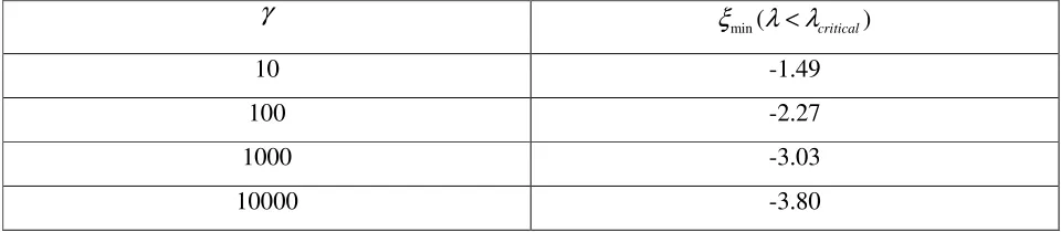
and the normalized potentialξ. We can compute theminimum value of normalized potential required to ensure the validity of the condition
λ λ
< critical with1.889
critical
λ
= for a givenγ
value. For normalized potential values more negative than this the [image:6.612.66.546.355.460.2]discriminant will not be positive. The results of the required computation is presented in table 1 below. This calculation in fact defines a lower bound for the potential which must be applied to ensure that the condition of rapid homogeneous kinetics is met.
Table 1. Dependence of normalized potential on reaction/diffusion parameter
γ
min( critical)
ξ
λ λ
<10 -1.49
100 -2.27
1000 -3.03
10000 -3.80
Note also that for large values of λ, ∆ will be positive since as the normalized potential ξ increases
the
λ
3 term will decrease and eventually approach zero. We can also show that1/ 3
3 3
1 1
2 27 4 27
S λ λ
= − + −
and also
1/ 3
3 3
1 1
2 27 4 27
T λ λ
= − − −
and so the physically meaningful solution to eqn.20 is:
1/ 3 1/ 3
3 3 3 3
1/ 3 1 1 1 1
2 27 4 27 2 27 4 27 3
λ λ λ λ λ
Ψ = − + − + − − − −
(25)
And the expression for the normalized current takes the form:
3
1/ 3 1/ 3
3 3 3 3
1 1 1 1
2 3 4 3 2 3 4 3 3
λ λ λ λ λ
Ψ = − + − + − − − −
If we substitute the expression for λ outlined in eqn.19 into eqn.26 we obtain an explicit expression for the normalized current versus potential curve as desired.
Returning to the cubic equation illustrated in eqn.20 we can set 1/ 3
3 λ
Ψ = Ζ − and hence the cubic transforms to
3 2
1 0
3 3
λ λ
λ
Ζ − + Ζ − − =
(27)
Which simplifies to
3
0
α β
Ζ − Ζ − = (28)
Where we have set
2
3
3 2 1
27 λ α
λ β
=
= −
(29)
Provided that 27β2>4α3 then the cubic equation presented in eqn.28 will have one real and two
complex roots. Furthermore it can be shown that we can find ϑ such that
3/ 2
3 cosh
2 β ϑ
α
=
(30)
And we can find the real root given by
[
]
[
]
[
]
2
cosh / 3 3
2
cosh 3 2 cosh 3
3
α ϑ
λ
ϑ κ ϑ
Ζ =
= =
(31)
We can readily show that
2
3 3 3
1
3 3 3
1 2 1 2 1 2
cosh ln 1
2 2 2
κ κ κ
ϑ
κ κ κ
−
− − −
= = + −
(32)
where we have set
{
}
[ ]
{
1/ 3}
1
3 3 4 exp
3
κ =λ = γ −ξ (33)
Hence the normalized current response can be evaluated from
(
)
3{
(
[
]
)
}
32 cosh 3 1
κ κ ϑ
Ψ = Ζ − = − (34)
This is an alternative expression for the normalized current response and can be used to define the
voltammetric response when the explicit potential dependence of the κparameter is inputted via the
We now evaluate the half wave potential. We note that the normalized potential is defined as:
(
0)
0F
E E
RT
ξ = − = −θ θ , and when θ θ= 1/ 2, Ψ =1/ 2. Hence from eqn.20 we obtain that
(
)
3 1/ 3
1/ 3 2 / 3
1/ 2 0
1 3 1
exp 1
2 4γ θ θ 2
+ − − =
.This expression is readily shown to simplify to:
(
)
1/ 3 2 / 3
1/ 2 0
3 1 1
exp
4 2 2
θ θ
γ
− − =
, and so we obtain on further rearrangement the following expression for the half wave potential:
1/ 2 0
1 1 3
ln 2 ln
3 3 4
θ θ
γ
= + +
(35)
We note that since the reaction/diffusion parameter γ is always positive then the term ln 3 4
{
γ}
<0 and so for an oxidation process, θ1/ 2<θ0 and 1/ 2 1ln 3
d d θ
γ = − . Hence we predict that the half wave potential should be shifted to more negative values with increasing values of the reaction/diffusion parameter γ . This variation, computed from eqn.35 is presented in figure 1 and in semi-logarithmic format in figure 2. These results are in agreement with data previously reported by Compton and co-workers [5] who attacked the problem using numerical methods.
γ
0 2e+4 4e+4 6e+4 8e+4 1e+5
∆
θ
=
θ
1/2
−
θ
0-4.0 -3.5 -3.0 -2.5 -2.0 -1.5 -1.0
Figure 1. Variation of ∆ =θ θ1/ 2−θ0 with reaction/diffusion parameter γ for an EC2 process computed from eqn.35.
[image:8.612.111.404.386.599.2]
{
}
2
0 0
2 3 3 2
0 0
2 4
3
p v
pdp v dv
p v v p
γ
γ
=
= − +
∫
∫
(36)
We recall that 02 4 03 3
p ≅ γ v and so :
2
2 3
3/ 2
4 3 4
3 dv
p v
d dv
v d
γ χ
γ χ
= =
= −
(37)
Separating the variables and integrating produces the following expression for the concentration profile of the electro-generated reactant species B in the diffusion layer:
0
1 1
3
v v
γ χ
= + (38)
γ
1e+0 1e+1 1e+2 1e+3 1e+4 1e+5
∆
θ
=
θ 1/
2
−
θ 0
[image:9.612.160.444.284.551.2]-4.0 -3.5 -3.0 -2.5 -2.0 -1.5 -1.0
Figure 2. Presentation of eqn.35 in semi-logarithmic format. Furthermore since v=0 χ=1 then v0 3
γ
= − and so the concentration profile is given by
{
}
1
1 3 v
γ χ
= − (39)
From eqn.15 we also note that
3/ 2
0 0
0 0
4 3
dv du
p v
d d
γ
χ χ
= = − = −
Also we note that
[ ]
0 0
0
1 1 exp
du
u v
dχ ξ
= − = − −
(41)
From eqn. 40 and eqn.41 we immediately obtain
[ ]
3/ 2
0 0
4
exp 1 0
3 v v
γ
ξ
+ − − = (42)
The latter may be written in the following form
( )
0 3[ ]
( )
0 23 3
exp 0
4 4
v ξ v
γ γ
+ − − = (43)
The latter expression defines a cubic in v0 which may also be solved via procedures similar to those outlined earlier in the paper. This approach was adopted by Compton and co-workers [5].
2.4 Extension of analysis to a general mth order homogeneous reaction: the ECm process.
We now briefly discuss how the analysis developed in the present paper may be extended to a more general reaction sequence in which one has an initial rapid interfacial heterogeneous electron transfer reaction followed by a homogeneous chemical reaction which follows mth order kinetics with a rate constant k.
We focus specific attention on the homogeneous reaction step occurring within the diffusion layer of thickness δ involving the electro-generated reactant in which the reaction stoichiometry is:
Products
k
mB→
Again the reaction/diffusion equation takes the form:
2
2 0
m
d v m v
dχ − γ = (44)
Where we have defined the reaction/diffusion parameter in this case as:
( )
21
m
k a D δ
γ = ∞ − (45)
Proceeding as before we get
2
2
2 dv d v 2m vm dv
dχ χd = γ dχ (46)
Now again we note that
2 2
2
2
d dv dv d v
dχ dχ dχ χd
=
and we also note that 2 1 2 1
m m
d m dv
v m v
dv m d
γ
γ χ +
=
+
hence from eqn.46 we obtain:
(
)
2
1
2 1
m
d dv m dv
d v d
d d m d
γ
χ χ
χ χ χ
+
=
+
∫
∫
(47)
(
)
2 1 2 1 m dv m v K d m γ χ + = + + (48)
The integration constant K is obtained by appropriate use of the boundary conditions. When
1
1
1 v v 0 dv dv
d d
χ
χ χ
= = = =
and so 1
dv K
dχ
=
. If we can make the further assumption that
1 0 dv dχ ≅
then K =0 and we obtain from eqn.48 that
(
)
(1 ) 2
2 1 m dv m v d m γ χ + ≅ − + (49)
Specifically at χ =0 the current is given by
(
)
(1 )2 0 0 2 1 m dv m v d m γ χ +
Ψ = − =
+
(50)
We recall that u0= − Ψ1 hence
(
)
(1 )2
0 0 2 1 1 m m u v m γ + = −
+ . Furthermore from the Nernst equation at the
electrode surface we note u0 =v0exp
[ ]
−ξ
.Hence we obtain that:[ ]
0
1− Ψ =v exp −
ξ
(51)From eqn.50 we obtain that:
( ) ( ) 1 1 2 1 0 1 2 m m m v m
γ
+ + + = Ψ
(52)
Hence from eqn,51 and eqn.52 we obtain the following expression for the current versus potential
curve for a m th order reaction:
( )
( )
[ ]
1 1
2 1 1
1 exp
2
m
m m
m
γ
ξ
+ + +
− Ψ = Ψ −
(53)
This expression may be written as:
( )
[
]
2 1
exp * 1 0
m
ξ
+
Ψ + Ψ − − = (54)
Where we have introduced
1 2 * ln 1 1 m m m γ ξ = +ξ
+ + (55)
This expression is in agreement with a result first proposed by Amatore [12]. Specifically for m = 2 we note that eqn.52 reduces to eqn.16 and eqn.54 transforms to eqn.20 as indeed it should.
3. CONCLUSIONS
In the present paper an analysis of an EC2 reaction sequence involving a Nernstian interfacial
to be formulated in terms of a cubic equation. Two closed form analytical solutions to the cubic have been proposed using standard methodologies. The variation in half wave potential with a characteristic
reaction/diffusion parameter has been proposed. Finally the extension of the analysis to an ECP type
process has been demonstrated.
Acknowledgements
This work was supported by Enterprise Ireland (Grant number SC/2003/0049), IRCSET (Grant number SC/2002/0169) and the HEA-PRTLI Programme.
References
1. C.P. Andrieux and J.M. Saveant in Investigation of rates and mechanism of reactions . Part II.
(C.F. Bernasconi, Ed.,), 4th Edition, Techniques of Chemistry Series, Vol. VI, Wiley, New
York, 1986, Chapter 7, pp. 305-390.
2. A.J. Bard, L.R. Faulkner, Electrochemical Methods: Fundamentals and Applications, Wiley,
New York, 1980, Chapter 11, pp.429-487.
3. (a) J. Koutecky and R. Brdicka, Collect. Czech Chem. Commun., 12 (1947) 337 ; (b) P.
Delehay , S. Ora, J. Am. Chem. Soc., 82 (1960) 329 ; L.H.J. Tong, K. Liang and W.R. Ruby, J.
Electroanal. Chem., 13 (1967) 245 ; Z. Galus, R.N. Adams, J. Electroanal. Chem., 4 (1962) 248.
4. J. Ulstrup, Electrochim Acta., 13 (1968) 1717.
5. (a) R.G. Compton, D. Mason and P.R. Unwin, J. Chem. Soc. Faraday Trans.I. 84 (1988) 473 ;
(b) R.G. Compton, P.R. Unwin, J. Chem. Soc. Faraday Trans.I. 85 (1989) 1821.
6. P.N. Bartlett, V. Eastwick-Field, J. Chem. Soc. Faraday Trans.I. 89 (1993) 213.
7. L.S. Marcoux, R.N. Adams and S.W. Feldberg, J. Phys. Chem., 73 (1969) 2611.
8. W.J. Albery, Electrode Kinetics, Clarendon Press, Oxford, 1975, pp.51-53.
9. W.J. Albery and M.L. Hitchman, Ring-Disc Electrodes, Clarendon Press, Oxford, 1971, p.13.
10.H.T. Davis, Introduction to nonlinear differential and integral equations, Dover, New York,
1962, pp.194-197.
11.M.R. Spiegel, Mathematical Handbook, McGraw Hill, New York, 1968, pp.179-182.
12.C. Amatore, in Organic Electrochemistry, (H. Lund, M.M. Baizer, Eds.), 3rd Edition, Marcel
Dekker, New York, 1991, Chapter 2, pp.11-119.