Component-level study of a decomposition-based multi-objective optimizer on a limited evaluation budget

This is a repository copy of

Component-level study of a decomposition-based

multi-objective optimizer on a limited evaluation budget

.

White Rose Research Online URL for this paper:

http://eprints.whiterose.ac.uk/129995/

Version: Accepted Version

Proceedings Paper:

Jones, O., Oakley, J.E. and Purshouse, R. orcid.org/0000-0001-5880-1925 (2018)

Component-level study of a decomposition-based multi-objective optimizer on a limited

evaluation budget. In: Aquirre, H., (ed.) Proceedings of the Genetic and Evolutionary

Computation Conference (GECCO 2018). Genetic and Evolutionary Computation

Conference (GECCO 2018), 15-19 Jul 2018, Kyoto, Japan. ACM , pp. 689-696. ISBN

978-1-4503-5618-3

https://doi.org/10.1145/3205455.3205649

© 2018 The Authors. This is an author produced version of a paper subsequently

published in Proceedings of the Genetic and Evolutionary Computation Conference

(GECCO 2018). Uploaded in accordance with the publisher's self-archiving policy.

[email protected]

https://eprints.whiterose.ac.uk/

Reuse

Items deposited in White Rose Research Online are protected by copyright, with all rights reserved unless

indicated otherwise. They may be downloaded and/or printed for private study, or other acts as permitted by

national copyright laws. The publisher or other rights holders may allow further reproduction and re-use of

the full text version. This is indicated by the licence information on the White Rose Research Online record

for the item.

Takedown

If you consider content in White Rose Research Online to be in breach of UK law, please notify us by

multi-objective optimizer on a limited evaluation budget

Oliver P. H. Jones

Department of Automatic Control & Systems Engineering University of Sheffield, UK [email protected]

Jeremy E. Oakley

School of Mathematics & Statistics University of Sheffield, UK

[email protected]

Robin C. Purshouse

Department of Automatic Control & Systems Engineering University of Sheffield, UK [email protected]

ABSTRACT

Decomposition-based algorithms have emerged as one of the most popular classes of solvers for multi-objective optimization. Despite their popularity, a lack of guidance exists for how to configure such algorithms for real-world problems, based on the features or contexts of those problems. One context that is important for many real-world problems is that function evaluations are expensive, and so algorithms need to be able to provide adequate convergence on a limited budget (e.g. 500 evaluations). This study contributes to emerging guidance on algorithm configuration by investigating how the convergence of the popular decomposition-based optimizer MOEA/D, over a limited budget, is affected by choice of component-level configuration. Two main aspects are considered: (1) impact of sharing information; (2) impact of normalisation scheme. The empirical test framework includes detailed trajectory analysis, as well as more conventional performance indicator analysis, to help identify and explain the behaviour of the optimizer. Use of neigh-bours in generating new solutions is found to be highly disruptive for searching on a small budget, leading to better convergence in some areas but far worse convergence in others. The findings also emphasise the challenge and importance of using an appropriate normalisation scheme.

CCS CONCEPTS

•Computing methodologies→Optimization algorithms;•Theory of computation→Evolutionary algorithms;•Applied comput-ing→Multi-criterion optimization and decision-making;

KEYWORDS

MOEA/D, decomposition-based multi-objective optimization, com-ponent study, trajectory analysis

ACM Reference format:

Oliver P. H. Jones, Jeremy E. Oakley, and Robin C. Purshouse. 2018. Component-level study of a decomposition-based multi-objective optimizer on a limited evaluation budget. InProceedings of Genetic and Evolutionary Computation

Conference, Kyoto, Japan, July 15–19, 2018 (GECCO ’18),8 pages.

DOI:

1

INTRODUCTION

Multi-objective evolutionary algorithms (MOEAs) have come to be used widely throughout both the scientific and engineering commu-nities, and are typically classified in terms of the primary selection method used in the algorithm:Pareto-based,decomposition-based andindicator-based [3]. Most of the methods that have been de-veloped within each class typically assume that a large budget will

exist for evaluating candidate solutions as the optimization process progresses. In many optimizer benchmarking studies, a budget of tens or hundreds of thousands of evaluations is used – for example, the CEC’09 MOEA competition permitted 300,000 evaluations [16]. However, solution evaluation can be an expensive procedure for many real-world applications (RWAs), typically arising from the use of high-fidelity simulations or physical experiments. In the case of high-fidelity simulations, even if the computational costs of running the models can be overcome (e.g. by careful exploita-tion of high performance computing facilities) then other resource constraints often still remain (e.g. availability of software licenses). In this setting, it is inappropriate to assume that a budget of many thousands of evaluations will be available to the optimizer.

Faced with this issue, algorithm designers have sought to couple surrogate modelling techniques to the optimization process [7]. In a loose coupling, the surrogate model is estimated either before the optimization begins, or at scheduled points during the opti-mization process. In more tightly coupled schemes, the surrogate model becomes a key component of the optimizer itself. These latter schemes have found particular favour for optimization on very small budgets – typically regarded as between 100 and 500 evaluations [9]. The algorithms, such as ParEGO [8], are typically highly complex in nature, featuring large numbers of configurable parameters. It remains unclear how these parameters should be set for different types of RWA, or how the behaviour of the overall algorithm is related to the behaviour of the underpinning selection method.

In the present study, we focus on the behaviour of a representa-tive algorithm from one of the main classes of MOEA – specifically, we consider theMOEA/Dalgorithm [14] from the decomposition-based family of optimizers. Rather than study the algorithm as a monolithic entity, we adopt acomponent-based approachthat allows the impact of different aspects of the algorithm to be analysed in detail [1, 10, 11]. The focus is on how typical component choices that would need to be made when configuring an optimizer for a RWA affect optimizer behaviour over a small evaluation budget. In this way, we seek to contribute the first known analysis of de-composition components for small budgets, in isolation from the complexity of surrogate-based components – with a view to mak-ing some preliminary recommendations for how such a targeted decomposition-based algorithm should be configured.

GECCO ’18, July 15–19, 2018, Kyoto, Japan O.P.H. Jones et al.

in Section 5. Section 6 draws conclusions and indicates future directions for the research.

2

MOEA/D AND ITS COMPONENTS

TheMulti Objective Evolutionary Algorithm based on Decomposition

was first presented by Zhang and Li in 2007 [14]. The algorithm is based on the classical multi-objective optimization concept of defining different reference directions in objective-space, and then directing the optimization process along each of these directions. The main innovation in MOEA/D is that information isshared

between neighbouring reference directions during a single opti-mization run – rather than performing separate optiopti-mization runs for each direction in turn as was used in the classical methods. The underlying hypothesis is that there is some kind of relationship in the neighbourhood that makes the sharing of information useful for the neighbours concerned.

MOEA/D has proved to be a seminal MOEA, with many variants and alternative decomposition-based schemes now in existence. A tightly-coupled surrogate-based addition – MOEA/D-EGO – was proposed in 2010 [15] as an alternative to the earlier ParEGO algo-rithm which also used decomposition-based principles [8].

A number of studies have investigated configuration choices for MOEA/D, offering alternatives to the originals proposed in [14]. Parameters examined include choice of norm in the scalarising function [4, 6], weight vector specification [12], and neighbourhood size [17].

2.1

Components of MOEA/D

Within the implementation of MOEA/D there are four main stages that can be abstracted as components: (1) initialisation; (2) repro-duction; (3) improvement; (4) update. In addition to these aspects, a further area of interest is the normalisation operation used to enable non-commensurate objectives to be compared. An overview of each of these components is given below.

Initialisation.The first step that needs to be performed is to initialise the various parameters present within the MOEA/D al-gorithm. The algorithm begins by defining a set of weight vectors, which are evenly spread throughout the output space. The next step is to set up neighbourhoods which consists of the closestn

weight vectors to each weight vector. The final aspect that needs to be implemented within the initialisation is the creation of a set of initial points. Within the MOEA/D algorithm, these points are determined either randomly or through a problem-specific method. Reproduction.After initialisation, the optimizer loops through all of the reference directions. For each direction, the optimizer will select two weight vectors from that direction’s neighbourhood and use the points from those two reference directions to perform reproduction. The type of reproduction used by MOEA/D is simu-lated binary crossover (SBX), during which only one offspring is created. That offspring then has polynomial mutation applied to it. Improvement.The improvement stage is used to apply either a problem specific repair or improvement heuristic to the offspring point. This stage is useful as it can ensure that the acquired solution is feasible.

Update of neighbouring solutions. This section of the al-gorithm works on ensuring that newly found solutions are used

effectively. The new solution is compared to all other solutions re-lated to it through its neighbourhood. The comparison of whether the newly found solution is superior to existing solutions in the neighbourhood is performed by applying the scalarisation function associated to each neighbour’s reference direction.

Normalisation. While normalisation is not a separate stage specifically stated within the MOEA/D algorithm, it is still carried out and has an effect on the algorithm’s performance. In the basic description of the algorithm in the original MOEA/D paper [14] there was no normalisation undertaken prior to scalarisation. How-ever, normalisation was discussed in a separate analysis within the original paper to understand if improved performance could be achieved when working with disparately-scaled objectives. The normalisation is undertaken with respect to the ideal and nadir points. These points are estimated progressively from the solutions that have be found so far: the best values achieved for each objec-tive are taken as the current estimate of the ideal; the worst values achieved within the current best set of solutions across all reference directions are taken as the current estimate of the nadir.

2.2

Implementation of components

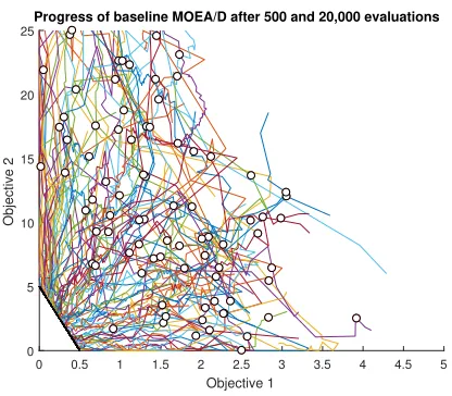
The baseline MOEA/D algorithm within this paper has been setup slightly differently to how it was described within Zhang and Li’s original paper. These variations are caused by the desire to test different aspects of the optimizer. The chosen initialisation method implemented throughout the paper is the widely used space-filling Latin hypercube sampling method. While this method does require the user to have knowledge of the limits of the input space, it ensures that the whole of the input space is well covered. In the baseline setup it is also assumed that the ideal and nadir points required for performing fixed normalisation are known to be the true values. The improvement step simply checks whether decision variables have moved outside of their bounds and, if so, sets them to the closest feasible boundary. It was assumed that components such as the neighbourhood, reproduction and updating are not implemented unless they are the aspect specifically under test. A representative trajectory plot for the baseline algorithm solving the test problem used in this study is shown in Figure 1. The pseudo-code for the algorithm is given in Algorithm 1.

Algorithm 1Component-level abstraction of MOEA/D

for1 : Total replicationsdo Initialise parameters Calculate neighbourhood

Acquire initial points using Latin Hypercube sampling for1 : Number of iterationsdo

for1 : Number of directionsdo for1 : Number of offspringdo

Optional component: Reproduction Perform Mutation

Improvement/Repair Evaluation

0 0.5 1 1.5 2 2.5 3 3.5 4 4.5 5

Objective 1

0 5 10 15 20 25

Objective 2

Progress of baseline MOEA/D after 500 and 20,000 evaluations

Figure 1: Trajectory plot for the baseline algorithm us-ing 100 reference directions and a budget of 20,000 evalua-tions (progress after 500 evaluaevalua-tions is shown by the circled points). Good convergence is observed for the larger budget.

3

COMPONENT INVESTIGATION

3.1

Areas of interest

While MOEA/D has many areas of interest that could be investi-gated, we focus on two key component choices for RWAs: the first of these is how the inclusion of information sharing through neigh-bourhoods affects the optimizer’s performance; the second area of interest is how different forms of normalization cause changes in the optimizer’s behaviour.

3.1.1 Baseline optimizer.The baseline configuration consists solely of a mutation component, with no reproduction, or update of, neighbouring solutions. Due to the budget limitations, a very modest number of reference directions has been chosen: 5 in total. The optimizer is run for 100 iterations, within each of which one evaluation is used for each of the 5 reference directions, leading to the total budget of 500 evaluations being exhausted. An elitist(µ+λ) strategy is used for selection across all variants of the algorithm. A (1+1)strategy is used in the baseline algorithm. Scalarisation is performed using the Tchbycheff norm.

3.1.2 Impact of sharing information. Three component config-urations consider the impact of sharing information between the different subproblems present within MOEA/D - all require the definition of a neighbourhood. The neighbourhood is defined as the adjacent reference directions. The first approach implements the update of neighbouring solutions component; the second im-plements SBX reproduction, with three solutions considered (the two parents are chosen at random from both the neighbourhood and the reference direction). The SBX distribution index is set to 20 as in the original MOEA/D paper [14]. The third setup consists of using the neighbourhood for both SBX reproduction and update of neighbouring solutions. This final configuration provide the greatest sharing of information between the different references

directions. As with the previous setups, a neighbourhood size of two is implemented in order to maintain consistency.

3.1.3 Impact of normalisation.One of the issues when perform-ing decomposition-based optimization on RWAs is that the location of the ideal point and nadir point, required for normalisation, are generally unknown. In many studies, an assumption is made about the points used for normalisation, such as is done in this paper dur-ing the assessment of shardur-ing of information. The choice of usdur-ing fixed known points for the ideal and nadir point is reasonable as it allows the impact of these neighbourhood features to be examined without having to simultaneously consider the impacts of using estimates of the ideal/nadir points. However, in order to test the impact of normalisation on the optimizer, different normalisation methods are applied to the most effective information sharing setup examined above.

Three alternative normalisation approaches are considered. The first variation is actually not to apply normalisation at all [5]. The use of adaptive normalisation is the second setup, in which new ideal and nadir estimates are obtained for each iteration of the optimizer. This is implemented in the same way as in the original MOEA/D paper. The final setup looks at whether using a portion of the evaluation budget to determine an approximate value of the ideal and nadir points could be beneficial. In order to determine these two points, a lexicographic optimization methodology is used with a(1+1)strategy. This first determines the minimum for one of the objectives, before minimising the second objective while maintaining the value found for the first.

3.2

Performance analysis

3.2.1 Test function.A modified version of the DTLZ1 function, initially presented in [2], has been chosen. It has been altered in order to make the objectives disparately scaled so that some form of normalisation might prove beneficial. The altered DTLZ1 function, referred to here as ‘DTLZ1alt’, is defined as:

Minimizef1= 1 2x1(1+д) Minimizef2=5(1−x1)(1+д)

д= h

5+ Õ

i∈ {2, . . .,6}

(xi−0.5)

2_−cos(2π(x

i−0.5))

i

Wherexi ∈ [0,1],i∈ {1, . . .,n},n=6.

(1) The test problem possesses a linear Pareto front, which stretches from the point[0,5]to[0.5,0]. Points on the front can be generated

by settingx2, . . .,6=0.5 and taking any choice forx1.

3.2.2 Performance indicator.The performance indicator used throughout the analysis is the inverted generational distance (IGD), which measures the quality of a non-dominated set in terms of both convergence and diversity simultaneously [13]. IGD calculates the average Euclidean distance between a set of evenly space points which lie along the Pareto front and the closest points to them from the current non-dominated set.

GECCO ’18, July 15–19, 2018, Kyoto, Japan O.P.H. Jones et al.

Independent Updating Reproduction Mixed 50

100 150 200

Integrated IGD

Boxplot showing IGD performance

Independent Updating Reproduction Mixed 0.2

0.4 0.6 0.8 1 1.2

Final IGD

Boxplot showing IGD achived after 500 evaluations

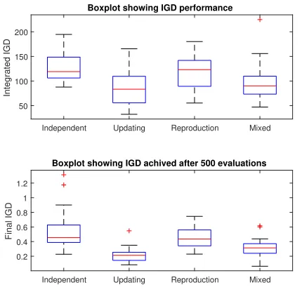
Figure 2: Boxplot showing how the use of neighbourhoods to share information between subproblems within the op-timizer impacts the IGD. It is evident that the inclusion of neighbourhoods for updating of neighbouring solutions has a positive impact on performance.

the optimizer will perform, each setup is run 31 times. Box plots are used to indicate the variation in performance, as well as median levels of attainment. In addition to the IGD obtained after 500 evaluations, anintegrated IGDis also considered, which considers the sum of the IGD obtained over the iterations of an optimizer run. The integrated measure provides some insight into how rapidly convergence is obtained, which is useful context if 500 is regarded as an upper limit on the number of permissible evaluations.

3.2.3 Subproblem convergence trajectories. In addition to the IGD metric, we also show the dynamic convergence in objective-space of the optimizer along each of the five reference directions. The trajectories are taken from the run of the optimizer associated with the median IGD result. These trajectories provide useful insight into the dynamic behaviour of the optimizer for different choices of information sharing or normalisation.

3.2.4 Significance testing.The statistical significance of the re-sults (at the 0.05 level) is determined using pairwise Wilcoxon rank-sum tests with Bonferroni correction. The test statistic used is the mean IGD performance for each algorithm after 500 evaluations.

4

RESULTS

4.1

Impact of sharing information

The results of implementing the different methods for information sharing can be observed in Figure 2. All relative rankings of algo-rithms implied by the lower boxplots are statistically significant, except between the independent and reproduction configurations, where no difference in mean performance could be confirmed.

0 50 100 150 200 250 300 350 400 450 500

Number of evaluations

0 0.5 1 1.5 2 2.5 3 3.5 4 4.5 5

IGD

IGD plot showing the effects of information sharing

Independent Updating SBX reproduction Mixed methods

Figure 3: Plot showing how the median IGD for different se-tups progresses over iterations of the optimizer. The positive impact of updating is clearly visible for the majority of the evaluation budget

When the subproblems are performed independently, the per-formance of the optimizer appears not to be particularly good with its final IGD achieving a median value of about 0.45. When the updating of neighbouring solutions component is included, a large positive impact on the optimizer’s performance is evident – with the optimizer achieving a median final IGD of about 0.21. Another point of interest with this setup is that the integrated IGD implies that it was also a lot faster to reduce its IGD, and so could prove to be a good option if there were the possibility that the optimizer would need to stop early. The use of reproduction without the update of neighbouring solutions does not improve the optimizer’s perfor-mance. While it produces an equivalent median final IGD when no information sharing was used, it possesses a worse integrated IGD. This can be more clearly seen in Figure 3 which shows the median runs based on the integrated IGD. The final setup examined is the one using a mix of SBX and updating neighbouring solutions. While this setup does perform better than that of either using the independent setup or SBX reproduction, it does not outperform the setup using just the update of neighbouring solutions.

0 0.5 1 1.5 2 2.5 3 3.5 4 4.5 5 Objective 1

0 5 10 15 20 25

Objective 2

DTLZ1alt optimized using independent optimization

(a) Independent

0 0.5 1 1.5 2 2.5 3 3.5 4 4.5 5 Objective 1

0 5 10 15 20 25

Objective 2

DTLZ1alt optimized using a neighbourhood size of two and updating neighbouring solutions

(b) Updating

0 0.5 1 1.5 2 2.5 3 3.5 4 4.5 5 Objective 1

0 5 10 15 20 25

Objective 2

DTLZ1alt optimized using a neighbourhood size of two and SBX reproduction

(c) Reproduction

0 0.5 1 1.5 2 2.5 3 3.5 4 4.5 5 Objective 1

0 5 10 15 20 25

Objective 2

DTLZ1alt optimized using a neighbourhood size of two with both SBX reproduction and updating of neighbouring solutions

(d) Mixed

Figure 4: Trajectory plots of the median runs, based on the integrated IGD. The inclusion of neighbourhoods causes clustering and rapid initial movement.

close to the Pareto front, as they remain clustered together. Finally, Figure 4(d) shows the effects of using a mixture of reproduction and updating the neighbouring solutions. Similar to before, the points progress down towards the Pareto front while being gath-ered together; once they reach the front they try and spread across it, but only have limited success.

4.2

Impact of normalisation

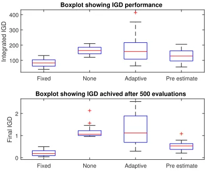
The results of testing the impact of applying different normalisa-tion methods are presented within the boxplots in Figure 5. As previously, all relative rankings of algorithms implied by the lower boxplots are statistically significant, except for the comparison between the adaptive approach and no normalisation, where no

GECCO ’18, July 15–19, 2018, Kyoto, Japan O.P.H. Jones et al.

Fixed None Adaptive Pre estimate 100

200 300 400

Integrated IGD

Boxplot showing IGD performance

Fixed None Adaptive Pre estimate 0

1 2

Final IGD

Boxplot showing IGD achived after 500 evaluations

Figure 5: Boxplot showing how normalisation affects IGD performance. Of interest is how reserving a portion of the budget for estimated ideal and nadir points greatly improves performance.

The last method considered was to pre-determine the ideal and nadir points before commencing optimization. It was determined that 80 evaluations were needed for each objective in order to estimate an acceptable ideal point and a further 40 were needed for each to get a suitable nadir point. The median values found for the ideal and nadir after the search was run are [0, 0.0683] and [0.9134, 8.4708] respectively. During testing, it was determined that the improvement gained with additional evaluations did not balance the loss in performance due to fewer iterations of the optimizer. Going back to Figure 5 it can be seen that when the predetermined estimates for the ideal and nadir points are used, the integrated IGD is improved while the final IGD was superior to that of either adaptive normalization or when no normalization was used.

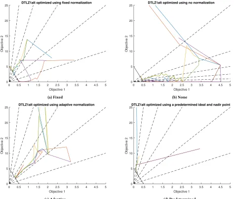
Looking at Figure 6, the trajectory plots of the median runs can be seen. In each of the four subplots, the dashed lines indicate the reference directions. In (a), (b) and (d) the reference directions represent those that the optimizer is using. In (c) the reference directions shown are the best ones that could be found, as they change during each iteration for adaptive normalisation. Figure 6(a) shows the fixed normalisation, with the trajectories moving down towards the front in the same manner as seen before. In Figure 6(b), when no normalization is applied, all of the trajectories head down towards the first objective axis before starting to move in towards the Pareto front. As the reference directions are evenly spaced across the objective space, they focus on the lower half of the Pareto front. In Figure 6(c) all of the trajectories move together before progressing down to the front, where they do not spread out. The final subplot, where the previously estimated ideal and nadir point are used, shows the points moving towards the front quickly before spreading out and managing to reach three of the reference directions (due to the points initialising close together, it is difficult to see their movement within this particular plot).

4.3

Interesting variants

There were a selection of interesting variants discovered during the process of testing. The first of which is when five offspring are used instead of just one. When implemented, it implies running the optimizer for only 20 iterations, so as to use the same number of evaluations in total as before. It can be seen in Figure 7 that, when compared to running the optimizer independently with one offspring, the trajectories obtained are much smoother. The erratic behaviour caused by the optimizer going back on itself is also almost entirely absent. This demonstrates how the addition of extra offspring allow for better directed convergence. When compared to the performance of using only a single offspring, equivalent median IGD was achieved.

The second interesting variant to be examined was discovered when running the optimizer with four neighbours and SBX re-production with no update of neighbouring solutions. Using four neighbours meant that points from any of the subproblems had a chance of being selected during the reproduction step. The median result of running this setup can be seen in Figure 8. All of the differ-ent trajectories are pulled together, almost to a single point, before attempting to spread out. The rate at which they can separate out is negatively impacted by the use of SBX.

5

DISCUSSION

It is evident that the sharing of information in a decomposition-based optimizer, through the use of neighbourhoods, between the different subproblems, can have a substantial impact on the opti-mizer’s performance. The clearest example of this was observed when the component for updating the neighbourhood solutions was used. From the trajectory plot it was seen that the compo-nent enabled rapid improvement by jumping to more advantageous point in objective-space. Updating the neighbourhood solutions also allowed the solutions to spread out once they were close to the Pareto front.

While it has often been shown that the use of reproduction (or recombination) can aid optimizer performance, this appears to be invalid in the context of a small number of reference directions. The use of reproduction does initially seem to help in moving the solutions down towards the Pareto front; however once they arrive their progress comes to an almost complete stop. A likely reason for this is that while only two neighbours are being used, this actually constitutes a sizeable region of the Pareto front. In most problems a much larger number of reference directions are used, such as the 150 to 250 reference directions used in the original MOEA/D study [14]. In an exploratory analysis using a ‘limited’ evaluation budget, the authors still used 20 reference directions and 250 iterations, which is a total evaluation budget that is an order of magnitude greater than that considered in this and other limited budget studies. Where a larger budget is available, any unhelpful effects of SBX reproduction are lessened due to the smaller distances between ref-erence directions (see Figure 1). Using both SBX reproduction and the update of neighbourhood solutions together proved to be unsat-isfactory, producing a worse IGD than the update of neighbouring solutions did on its own.

0 0.5 1 1.5 2 2.5 3 3.5 4 4.5 5 Objective 1

0 5 10 15 20 25

Objective 2

DTLZ1alt optimized using fixed normalization

(a) Fixed

0 0.5 1 1.5 2 2.5 3 3.5 4 4.5 5 Objective 1

0 5 10 15 20 25

Objective 2

DTLZ1alt optimized using no normalization

(b) None

0 0.5 1 1.5 2 2.5 3 3.5 4 4.5 5 Objective 1

0 5 10 15 20 25

Objective 2

DTLZ1alt optimized using adaptive normalization

(c) Adaptive

0 0.5 1 1.5 2 2.5 3 3.5 4 4.5 5 Objective 1

0 5 10 15 20 25

Objective 2

DTLZ1alt optimized using a predetermined ideal and nadir point

(d) Predetermined

Figure 6: Trajectory plots of the median runs using different normalisation methods, based on the integrated IGD. It is evident that lacking good estimates of the ideal and nadir points greatly compromises the ability of a decomposition-based optimizer to find the Pareto front.

performance, it is unrealistic for most RWAs as both the ideal and nadir points are unlikely to be known in advance. The next option of simply using no normalisation proved to be worse for the chosen disparately scaled test problem. This was due to the reference directions forcing points to one side of the front. The option of using adaptive normalisation, which is a more feasible option, proved to have a poor IGD value while also possessing a high degree of variability, which is undesirable. Using pre-estimation provided a considerable improvement over all but fixed normalisation, even though it reduced the subsequent number of evaluations available to the optimizer.

While our findings have implications for the design and con-figuration of decomposition-based optimizers, it is important to acknowledge that only a single problem instance was used in the

analysis. Generalisation of findings to other classes of problem should be handled cautiously pending further experimental studies.

6

CONCLUSION

GECCO ’18, July 15–19, 2018, Kyoto, Japan O.P.H. Jones et al.

0 0.5 1 1.5 2 2.5 3 3.5 4 4.5 5

Objective 1

0 5 10 15 20 25

Objective 2

DTLZ1alt optimized using five offspring

Figure 7: Trajectory plot when five offspring are generated, in the absence of information sharing components. Note the smoother trajectories approaching the Pareto front, when compared to the previous single offspring configurations.

0 0.5 1 1.5 2 2.5 3 3.5 4 4.5 5

Objective 1

0 5 10 15 20 25

Objective 2

DTLZ1alt optimized using a neighbourhood size of four for SBX reproduction

Figure 8: Trajectory plot when four neighbours are used for SBX and there is no update of neighbouring solutions. The points cluster together, affecting the overall ability of the optimizer to find the Pareto front.

inadvisable. When considering what form of normalisation to use, it was found that using a subset of the evaluation budget to gain an estimate of the ideal and nadir points for normalisation proved more effective than the conventional adaptive scheme, and achieved close to the performance of the ideal, but infeasible, approach of knowing the correct normalisation parameters in advance.

The next stage for this work is to extend the analysis to an ex-panded set of benchmark problems and to more complex, surrogate-based optimizers that rely on a decomposition approach, e.g. the seminal ParEGO algorithm [8].

Acknowledgments. This work was supported by Jaguar Land Rover and the EPSRC grant EP/L025760/1 as part of the jointly fundedProgramme for Simulation Innovation. The first author ac-knowledges EPSRC studentship support.

REFERENCES

[1] Leonardo C. T. Bezerra, Manuel L´opez-Ib´a ˜nez, and Thomas St¨utzle. 2015. Com-paring Decomposition-Based and Automatically Component-Wise Designed

Multi-Objective Evolutionary Algorithms. InEvolutionary Multi-Criterion

Opti-mization, EMO 2015 Part I. 396–410.

[2] Kalyanmoy Deb, Lothar Thiele, Marco Laumanns, and Eckart Zitzler. 2005.

Scal-able test problems for evolutionary multiobjective optimization.Evolutionary

Multiobjective Optimization. Theoretical Advances and Applications(2005), 105– 145.

[3] Ioannis Giagkiozis, Robin C. Purshouse, and Peter J. Fleming. 2015. An overview

of population-based algorithms for multi-objective optimisation.International

Journal of Systems Science46, 9 (2015), 1572–1599.

[4] Hisao Ishibuchi, Naoya Akedo, and Yusuke Nojima. 2013. A study on the spec-ification of a scalarizing function in MOEA/D for many-objective knapsack

problems. InInternational Conference on Learning and Intelligent Optimization.

231–246.

[5] Hisao Ishibuchi, Ken Doi, and Yusuke Nojima. 2017. On the effect of

normaliza-tion in MOEA/D for multi-objective and many-objective optimizanormaliza-tion.Complex

& Intelligent Systems3, 4 (2017), 279–294.

[6] Hisao Ishibuchi, Yuji Sakane, Noritaka Tsukamoto, and Yusuke Nojima. 2010.

Simultaneous use of different scalarizing functions in MOEA/D. InProceedings of

the 12th Annual Conference on Genetic and Evolutionary Computation. 519–526. [7] Yaochu Jin. 2011. Surrogate-assisted evolutionary computation: Recent advances

and future challenges.Swarm and Evolutionary Computation1, 2 (2011), 61–70.

[8] Joshua Knowles. 2006. ParEGO: a hybrid algorithm with on-line landscape

approximation for expensive multiobjective optimization problems.IEEE

Trans-actions on Evolutionary Computation10, 1 (2006), 50–66.

[9] Joshua Knowles and Evan J. Hughes. 2005. Multiobjective optimization on a

budget of 250 evaluations.Lecture Notes in Computer Science(2005), 176–190.

[10] Marco Laumanns, Eckart Zitzler, and Lothar Thiele. 2001. On the Effects of Archiving, Elitism, and Density Based Selection in Evolutionary Multi-Objective

Optimization. InProceedings of the First International Conference on Evolutionary

Multi-Criterion Optimization (EMO 2001). 181–196.

[11] Robin C. Purshouse and Peter J. Fleming. 2002. Why use Elitism and Sharing

in a Multi-Objective Genetic Algorithm?. InProceedings of the 2002 Genetic and

Evolutionary Computation Conference (GECCO 2002). 520–527.

[12] Yutao Qi, Xiaoliang Ma, Fang Liu, Licheng Jiao, Jianyong Sun, and Jianshe Wu.

2014. MOEA/D with adaptive weight adjustment.Evolutionary Computation22,

2 (2014), 231–264.

[13] Margarita R. Sierra and Carlos A. Coello Coello. 2004. A new multi-objective particle swarm optimizer with improved selection and diversity mechanisms.

Technical Report of CINVESTAV-IPN(2004).

[14] Qingfu Zhang and Hui Li. 2007. MOEA/D: A multiobjective evolutionary

algo-rithm based on decomposition.IEEE Transactions on Evolutionary Computation

11, 6 (2007), 712–731.

[15] Qingfu Zhang, Wudong Liu, Edward Tsang, and Botond Virginas. 2010. Expensive

multiobjective optimization by MOEA/D with Gaussian Process model.IEEE

Transactions on Evolutionary Computation14, 3 (2010), 456–474.

[16] Qingfu Zhang, Aimin Zhou, Shizheng Zhao, Ponnuthurai N. Suganthan, Wudong

Liu, and Santosh Tiwari. 2009.Multiobjective optimization test instances for the

CEC 2009 special session and competition. Technical Report. University of Essex. [17] Shi-Zheng Zhao, Ponnuthurai N. Suganthan, and Qingfu Zhang. 2012.

Decomposition-based multiobjective evolutionary algorithm with an

ensem-ble of neighborhood sizes.IEEE Transactions on Evolutionary Computation16, 3