This is a repository copy of
E8 spectral curves
.
White Rose Research Online URL for this paper:
http://eprints.whiterose.ac.uk/152157/
Version: Submitted Version
Article:
Brini, A. orcid.org/0000-0002-3758-827X (Submitted: 2017) E8 spectral curves. arXiv.
(Submitted)
© 2017 The Author(s). For reuse permissions, please contact the Author(s).
[email protected] https://eprints.whiterose.ac.uk/
Reuse
Items deposited in White Rose Research Online are protected by copyright, with all rights reserved unless indicated otherwise. They may be downloaded and/or printed for private study, or other acts as permitted by national copyright laws. The publisher or other rights holders may allow further reproduction and re-use of the full text version. This is indicated by the licence information on the White Rose Research Online record for the item.
Takedown
If you consider content in White Rose Research Online to be in breach of UK law, please notify us by
E8 SPECTRAL CURVES
ANDREA BRINI
Abstract. I provide an explicit construction of spectral curves for the affine E8 relativistic Toda chain. Their closed form expression is obtained by determining the full set of character relations in the representation ring of E8 for the exterior algebra of the adjoint representation; this is in turn employed to provide an explicit construction of both integrals of motion and the action-angle map for the resulting integrable system.
I consider two main areas of applications of these constructions. On the one hand, I consider the resulting family of spectral curves in the context of the correspondences between Toda systems, 5d Seiberg–Witten theory, Gromov–Witten theory of orbifolds of the resolved conifold, and Chern– Simons theory to establish a version of the B-model Gopakumar–Vafa correspondence for the slN
Lˆe–Murakami–Ohtsuki invariant of the Poincar´e integral homology sphere to all orders in 1/N. On the other, I consider a degenerate version of the spectral curves and prove a 1-dimensional Landau– Ginzburg mirror theorem for the Frobenius manifold structure on the space of orbits of the extended affine Weyl group of type E8 introduced by Dubrovin–Zhang (equivalently, the orbifold quantum cohomology of the type-E8polynomialCP1orbifold). This leads to closed-form expressions for the flat co-ordinates of the Saito metric, the prepotential, and a higher genus mirror theorem based on the Chekhov–Eynard–Orantin recursion. I will also show how the constructions of the paper lead to a generalisation of a conjecture of Norbury–Scott to ADEP1-orbifolds, and a mirror of the Dubrovin–Zhang construction for all Weyl groups and choices of marked roots.
1. Introduction 2
1.1. Context 2
1.2. What this paper is about 4
Acknowledgements 7
2. The E8 and Ec8 relativistic Toda chain 7
2.1. Notation 7
2.2. Kinematics 9
2.3. Dynamics 11
2.4. The spectral curve 11
2.5. Spectral vs parabolic vs cameral cover 16
3. Action-angle variables and the preferred Prym–Tyurin 18
3.1. Algebraic action-angle integration 19
3.2. The Kanev–McDaniel–Smolinsky correspondence 20
3.3. Hamiltonian structure and the spectral curve differential 25
4. Application I: gauge theory and Toda 31
4.1. Seiberg–Witten, Gromov–Witten and Chern–Simons 31
4.2. On the Gopakumar–Vafa correspondence for the Poincar´e sphere 41
4.3. Some degeneration limits 50
1
5. Application II: theEc8 Frobenius manifold 55
5.1. Dubrovin–Zhang Frobenius manifolds and Hurwitz spaces 55
5.2. A 1-dimensional LG mirror theorem 61
5.3. General mirrors for Dubrovin–Zhang Frobenius manifolds 67
5.4. PolynomialP1 orbifolds at higher genus 69
Appendix A. Proof of Proposition 3.1 73
Appendix B. Some formulas for the e8 and e(1)8 root system 74
B.1. On the minimal orbit of W 75
B.2. The binary icosahedral group ˜I 77
B.3. The prepotential ofXee8,3 77
Appendix C. ∧•e8 and relations inR(E8): an overview of the results of [23] 80
References 82
Contents
1. Introduction
Spectral curves have been the subject of considerable study in a variety of contexts. These are moduli spaces S of complex projective curves endowed with a distinguished pair of meromorphic abelian differentials and a marked symplectic subring of their first homology group; such data define (one or more) families of flat connections on the tangent bundle of the smooth part of moduli space. In particular, a Frobenius manifold structure on the base of the family, a dispersionless integrable hierarchy on its loop space, and the genus zero part of a semi-simple CohFT are then naturally defined in terms of periods of the aforementioned differentials over the marked cycles; a canonical reconstruction of the dispersive deformation (resp. the higher genera of the CohFT) is furthermore determined byS through the topological recursion of [49].
The one-line summary of this paper is that I offer two constructions (related to Points (II) and (IV) below) and two isomorphisms (related to Points (III), (V) and (VI)) in the context of spectral curves with exceptional gauge symmetry of type E8.
1.1. Context. Spectral curves are abundant in several problems in enumerative geometry and mathematical physics. In particular:
(I) in the spectral theory of finite-gap solutions of the KP/Toda hierarchy, spectral curves arise as the (normalised, compactified) affine curve in C2 given by the vanishing locus of the
Burchnall–Chaundy polynomial ensuring commutativity of the operators generating two dis-tinguished flows of the hierarchy; the marked abelian differentials here are just the differen-tials of the two coordinate projections onto the plane. In this case, to each smooth point in moduli space with fibre a smooth Riemann surface Γ there corresponds a canonical theta-function solution of the hierarchy depending ong(Γ) times, and the associated dynamics is encoded into a linear flow on the Jacobian of the curve;
(II) in many important cases, this type of linear flow on a Jacobian (or, more generally, a princi-pally polarised Abelian subvariety thereof, singled out by the marked basis of 1-cycles on the curve) is a manifestation of the Liouville–Arnold dynamics of an auxiliary, finite-dimensional integrable system. Coordinates in moduli space correspond to Cauchy data – i.e., initial values of involutive Hamiltonians/action variables – and flow parameters are given by linear coordinates on the associated torus;
(III) all the action has hitherto taken place at a fixed fibre over a point in moduli space; how-ever additional structures emerge once moduli are varied by considering secular (adiabatic) deformations of the integrals of motions via the Whitham averaging method. This defines a dynamics on moduli space which is itself integrable and admits aτ-function; remarkably, the logarithm of theτ-function satisfies the big phase-space version of WDVV equations, and its restriction to initial data/small phase space defines an almost-Frobenius manifold structure on the moduli space;
(IV) from the point of view of four dimensional supersymmetric gauge theories with eight super-charges, the appearance of WDVV equations for the Whithamτ-function is equivalent to the constraints of rigid special K¨ahler geometry on the effective prepotential; such equivalence is indeed realised by presenting the Coulomb branch of the theory as a moduli space of spectral curves, the marked differentials giving rise to the the Seiberg–Witten 1-form, the BPS central charge as the period mapping on the marked homology sublattice, and the prepotential as the logarithm of the Whitham τ-function;
(V) in several cases, the Picard–Fuchs equations satisfied by the periods of the SW differential are a reduction of the GKZ hypergeometric system for a toric Calabi–Yau variety, whose quantum cohomology is then isomorphic to the Frobenius manifold structure on the moduli of spectral curves. What is more, spectral curve mirrors open the way to include higher genus Gromov–Witten invariants in the picture through the Chekhov–Eynard–Orantin topological recursion: a universal calculus of residues on the fibres of the familyS, which is recursively determined by the spectral data. This provides simultaneously a definition of a higher genus topological B-model on a curve, a higher genus version of local mirror symmetry, and a dispersive deformation of the quasi-linear hierarchy obtained by the averaging procedure;
(VI) in some cases, spectral curves may also be related to multi-matrix models and topological gauge theories (particularly Chern–Simons theory) in a formal 1/N expansion: for fixed ’t Hooft parameters, the generating function of single-trace insertion of the gauge field in the planar limit cuts out a plane curve inC2. The asymptotic analysis of the matrix model/gauge
theory then falls squarely within the above setup: the formal solution of the Ward identities of the model dictates that the planar free energy is calculated by the special K¨ahler geometry relations for the associated spectral curve, and the full 1/N expansion of connected multi-trace correlators is computed by the topological recursion.
A paradigmatic example is given by the spectral curves arising as the vanishing locus for the characteristic polynomial of the Lax matrix for the periodic Toda chain withN+1 particles. In this
case (I) coincides with the theory ofN-gap solutions of the Toda hierarchy, which has a counterpart (II) in the Mumford–van Moerbeke algebro-geometric integration of the Toda chain by way of a flow on the Jacobian of the curves. In turn, this gives a Landau–Ginzburg picture for an (almost) Frobenius manifold structure (III), which is associated to the Seiberg–Witten solution of N = 2 pure SU(N+ 1) gauge theory (IV). The relativistic deformation of the system relates the Frobenius manifold above to the quantum cohomology (V) of a family of toric Calabi–Yau threefolds (for
N = 1, this is KP1×P1), which encodes the planar limit of SU(M) Chern–Simons–Witten invariants
on lens spaces L(N + 1,1) in (VI).
1.2. What this paper is about. A wide body of literature has been devoted in the last two decades to further generalising at least part of this web of relations to a wider arena (e.g. quiver gauge theories). A somewhat orthogonal direction, and one where the whole of (I)-(VI) have a concrete generalisation, is to consider the Lie-algebraic extension of the Toda hierarchy and its relativistic counterpart to arbitrary root systems R associated to semi-simple Lie algebras, the standard case corresponding to R = AN. Constructions and proofs of the relations above have
been available for quite a while for (II)-(IV) and more recently for (V)-(VI), in complete generality except for one, single, annoyingly egregious example: R= E8, whose complexity has put it out of
reach of previous treatments in the literature. This paper grows out of the author’s stubborness to fill out the gap in this exceptional case and provide, as an upshot, some novel applications of Toda spectral curves which may be of interest for geometers and mathematical physicists alike. As was mentioned, the aim of the paper is to provide two main constructions, and prove two isomorphisms, as follows.
Construction 1: The first construction fills the gap described above by exhibiting closed-form expressions for arbitrary moduli of the family of curves associated to the relativistic Toda chain of type Eb8 for its sole quasi-minuscule representation – the adjoint. This is
achieved in two steps: by determining the dependence of the regular fundamental characters of the Lax matrix on the spectral parameter, and by subsequently computing the polynomial character relations in the representation ring of E8 (viewed as a polynomial ring over the
fundamental characters) corresponding to the exterior powers of the adjoint representation. The last step, which is of independent representation-theoretic interest, is the culmination of a computational tour-de-force which in itself is beyond the scope of this paper, and will find a detailed description in [23]; I herein limit myself to announce and condense the ideas of [23] into the 2-page summary given in Appendix C, and accompany this paper with a
Mathematica package1 containing the solution thus achieved. As an immediate spin-off I obtain the generating function of the integrable model (in the language of [55]) as a function of the basic involutive Hamiltonians attached to the fundamental weights, and a family of spectral curves as its vanishing locus. In the process, this yields a canonical set of integrals of motion in involution in cluster variables and in Darboux co-ordinates for the integrable
1This is available athttp://tiny.cc/E8SpecCurve. Part of the complexity is reflected in the size of the compressed
data containing the final solution (∼180Mb – should the reader wish to have a closer look at this, they should be aware that this unpacks to binary files and aMathematicanotebook that are collectively 5x this size).
system on a special double Bruhat cell of the coextended Poisson–Lie loop group Ec8 #
, which, by analogy with the case of A-series, I call “the relativisticb Ec8 Toda chain”, and
whose dynamics is solved completely by the preceding construction.
Construction 2: The previous construction gives the first element in the description of the spectral curve – a family of plane complex algebraic curves, which are themselves integrals of motion. The next step determines the three remaining characters in the play, namely the two marked Abelian differentials and the distinguished sublattice of the first homology of the curves; this goes hand in hand with the construction of appropriate action–angle variables for the system. The ideology here is classical [37, 60, 68, 87, 117] in the non-relativistic case, and its adaptation to the relativistic setting at hand is straightforward: I identify the phase space of the Toda system with a fibration over the Cartan torus of E8 (timesC⋆) by
Abelian varieties, which are Prym–Tyurin sub-tori of the spectral curve Jacobian. These are selected by the curve geometry itself, due to an argument going back to Kanev [68], and the Liouville–Arnold flows linearise on them. The Hamiltonian structure inherited from the embedding of the system into a Poisson–Lie–Bruhat cell translates into a canonical choice of symplectic form on the universal family of Prym–Tyurins, and it pins down (up to canonical transformation) a marked pair of Abelian third kind differentials on the curves.
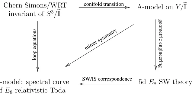
Altogether, the family of curves, the marked 1-forms, and the choice of preferred cycles lead to the assignment of a set of Dubrovin–Krichever data(Definition 3.1) to the family of spectral curves. Armed with this, I turn to some of the uses of Toda spectral curves in the context of Fig. 1.
conifold transition
geometric engineering
SW/IS correspondence
loop equations
mirror symmetry
5dE8 SW theory
Chern-Simons/WRT invariant ofS3/eI
B-model: spectral curve of E8 relativistic Toda
[image:6.612.175.493.420.580.2]A-model onY /eI
Figure 1. Duality web for the B-model on Toda spectral curves
Isomorphism 1: Toda spectral curves have long been proposed to encode the Seiberg–Witten solution of N = 2 pure gluodynamics in four dimensional Minkowski space [59, 85], as well as of its higher dimensional N = 1 parent theory on R4×S1 [94] in the relativistic case.
From the physics point of view, Constructions 1-2 provide the Seiberg–Witten solution for minimal, five-dimensional supersymmetric E8 Yang–Mills theory on R4×S1; and as the
latter should be related to (twisted) curve counts on an orbifold of the resolved conifold
Y = OP1(−1)⊕ OP1(−1) by the action of the binary icosahedral group ˜I, the same
con-struction provides a conjectural 1-dimensional mirror concon-struction for the orbifold Gromov– Witten theory of these targets, as well as to its large N Chern–Simons dual theory on the Poincar´e sphere S3/˜I≃Σ(2,3,5) [3, 15, 58, 99]. I do not pursue here the proof of either the bottom horizontal (SW/integrable systems correspondence) or the diagonal (mirror sym-metry) arrow in the diagram of Fig. 1, although it is highlighted in the text how having access to the global solution on its Coulomb branch allows to study particular degenera-tion limits of the soludegenera-tion corresponding to superconformal (maximally Argyres–Douglas) points where mutually non-local dyons pop up in the massless spectrum, and limiting ver-sions of mirror symmetry for the Toda curves in Isomorphism 2 below are also considered. What I do prove instead is a version of the vertical arrow, completing results in a previous joint paper with Borot [15]: namely, that the Chern–Simons/Reshetikhin–Turaev–Witten invariant of Σ(2,3,5) restricted to the trivial flat connection (the Lˆe–Murakami–Ohtsuki invariant), as well as the quantum invariants of fibre knots therein in the same limit and for arbitrary colourings, are computed to all orders in 1/N from the Chekhov–Eynard–Orantin topological recursion on a suitable subfamily of Ec8 relativistic Toda spectral curves. As in
[15], the strategy resorts to studying the trigonometric eigenvalue model associated to the LMO invariant of the Poincar´e sphere at large N and to prove that the planar resolvent is one of the meromorphic coordinate projections of a plane curve in (C⋆)2, which is in turn
shown to be the affine part of the spectral curve of the cE8 relativistic Toda chain.
Isomorphism 2: I further consider two meaningful operations that can be performed on the spectral curve setup of Construction 1-2. The first is to take a degeneration limit to the leaf where the natural Casimir function of the affine Toda chain goes to zero; this corresponds to the restriction to degree-zero orbifold invariants on the top-right corner of Fig. 1, and to the perturbative limit of the 5D prepotentials of the bottom-right corner. The second is to replace one of the marked Abelian integrals with their exponential; this is a version of Dubrovin’s notion of (almost)-duality of Frobenius manifolds [41].
I conjecture and prove that the resulting spectral curve provides a 1-dimensional Landau– Ginzburg mirror for the Frobenius manifold structure constructed on orbits of the extended affine Weyl group of type E8 by Dubrovin and Zhang [43]. Their construction depends on a
choice of simple root, and the canonical choice they take matches with the Frobenius man-ifold structure on the Hurwitz space determined by our global spectral curve. This extends to the first (and most) exceptional case the LG mirror theorems of [42] for the classical series; and it opens the way to formulate a precise conjecture for how the general case, encompassing general choices of simple roots in the Dubrovin–Zhang construction, should receive an analogous description in terms of Toda spectral curves for the corresponding Poisson–Lie group and twists thereof by the action of a Type I symmetry of WDVV (in the language of [39]). Restricting to the simply-laced case, this gives a mirror theorem for the quantum cohomology of ADE orbifolds of P1; our genus zero mirror statement then
lifts to an all-genus statement by virtue of the equivalence of the topological recursion with
Givental’s quantisation for R-calibrated Frobenius manifolds. This provides a version, for the ADE series, of statements by Norbury–Scott [46, 53, 96] for the Gromov–Witten theory of P1.
The two constructions and two isomorphisms above will find their place in Section 2, 3, 4 and 5 respectively. I have tried to give a self-contained exposition of the material in each of them, and to a good extent the reader interested in a particular angle of the story may read them independently (in particular Sections 4 and 5).
Acknowledgements. I would like to thank G. Bonelli, G. Borot, A. D’Andrea, B. Dubrovin, N. Orantin, N. Pagani, P. Rossi, A. Tanzini, Y. Zhang for discussions and correspondence on some of the topics touched upon in this paper, and H. Braden for bringing [86–88] to my attention during a talk at SISSA in 2015. For the calculations of Appendix C and [23], I have availed myself of cluster computing facilities at the Universit´e de Montpellier (Omega departmental cluster at IMAG, and the HPC@LR centreThau/Museinter-faculty cluster) and the compute cluster of the Department of Mathematics at Imperial College London. I am grateful to B. Chapuisat and especially A. Thomas for their continuous support and patience whilst these computations were carried out. This research was partially supported by the ERC Consolidator Grant no. 682603 (PI: T. Coates).
2. The E8 and Ec8 relativistic Toda chain
I will provide a succinct, but rather complete account of the construction of Lax pairs for the relativistic Toda chain for both the finite and affine E8 root system. This is mostly to fix notation
and key concepts for the discussion to follow, and there is virtually no new material here until Section 2.4. I refer the reader to [55, 98, 105, 114, 118] for more context, references, and further discussion. I will subsequently move to the explicit construction of spectral curves and the action-angle map for the affine E8 chain in Sections 2.4 and 3.
2.1. Notation. I will start by fixing some basic notation for the foregoing discussion; in doing so I will endeavour to avoid the uncontrolled profileration of subscripts “8” related to E8 throughout
the text, and stick to generic symbols instead (such asG for the E8 Lie group, gfor its Lie algebra,
and so on). I wish to make clear from the outset though that whilst many aspects of the discussion are general, the focus of this section is on E8 alone; the attentive reader will notice that some of
its properties, such as simply-lacedness, or triviality of the centre, are implicitly assumed in the formulas to follow.
Let then g , e8 denote the complex simple Lie algebra corresponding to the Dynkin diagram of
type E8 (Fig. 2). I will writeG = expgfor the corresponding simply-connected complex Lie group,
T = exphfor the maximal torus (the exponential of the Cartan algebrah⊂g), andW =NT/T for the Weyl group. I will also write Π ={α1, . . . , α8}for the set of simple roots (see e.g. (B.1)), and ∆,
∆∗, ∆(0), ∆± to indicate respectively the full root system, the non-vanishing roots, the zero roots,
and the negative/positive roots; the choice of splitting ∆± determines accordingly Borel subgroups
2 4
3
6 5 4 3 2 1
α0
α8
α2 α3 α4 α5 α6 α7
[image:9.612.103.514.73.168.2]α1
Figure 2. The Dynkin diagrams of type E8 and, superimposed in red, type E(1)8 ;
roots are labelled following Dynkin’s convention (left-to-right, bottom-to-top). The numbers in blue are the Dynkin labels for each vertex – for the non-affine roots, these are the components of the highest root in theα-basis.
B± intersecting at T. Each Borel realises G as a disjoint union of double cosets G =B±WB± = `
w∈WB±wB± = `
(w+,w−)∈W×W(B +w
+B+∩ B−w−B−) =: `(w+,w−)∈W×WCw+,w−, the double
Bruhat cells ofG. The Euclidean vector space (spanRΠ;h,i)⊂h∗ is a vector subspace ofh∗with an
inner product structure hβ, γi given by the dual of the Killing form; in particular, hαi, αji , Ci,jg
is the Cartan matrix (B.3). For a weight λ in the lattice Λw(G) , {λ ∈ h∗| hλ, αi ∈ Z}, I will
write Wλ = StabλW for the parabolic subgroup stabilised by λ; the action of W on weights is the
restriction of the coadjoint action onh∗; sinceZ(G) =ein our case, the weight lattice is isomorphic to the root lattice Λr(G) =ZhΠi ≃Λw(G). Corresponding to the choice of Π, Chevalley generators
{(hi ∈h, e±i ∈Lie(B±)|i∈Π}forg will be chosen satisfying
[hi, hj] = 0,
[hi, ej] = sgn(j)δi|j|ej,
[ei, e−i] = sgn(i)Cijghj,
(adei)1−C g
ijej = 0 for i+j6= 0. (2.1)
Accordingly, the correponding time-t flows on G lead to Chevalley generators Hi(t) = expthi, Ei(t) = exptei for the Lie group. Finally, I denote by R(G) the representation ring of G, namely
the free abelian group of virtual representations of G (i.e. formal differences), with ring structure given by the tensor product; this is a polynomial ringZ[ω] over the integers with generators given by the irreducible G-modules having ωi ∈ Λw(G) as their highest weights, where hωi, αji = δij.
Most of the notions (and notation) above carries through to the setting of the Kac–Moody group2 b
G = expg(1) where g(1) ≃ g⊗C[λ, λ−1]⊕Cc is the (necessarily untwisted, for g ≃ e8) affine Lie 2It should be noticed that, while in (2.1) passing fromhi toh′
i=PCijghj is an isomorphism of Lie algebras, the
same is not true in the affine setting as the Cartan matrix is then degenerate. Our discussion below sticks to the Lie algebra relations as written in (2.1), rather than their more common dualised form; in the affine setting, this substantial difference leads to the centrally coextended loop group instead of the more familiar central extension in Kac–Moody theory. In [55], this is stressed by employing the notationG# for the co-extended group; as I make clear from the outset in (2.1) what side of the duality I am sitting on, I somewhat abuse notation and denoteGbthe resulting Poisson–Lie group.
algebra corresponding toe8. In this case we adjoin the highest (affine) rootα0as in (B.2), leading to
the Dynkin diagram and Cartan matrix in Fig. 2 and (B.4). Elementsg∈Gbare linearq-differential polynomials in the spectral parameterλ; namely,g=M(λ)qλ∂λ, with the pointwise multiplication
rule leading to
g1g2 =M1(λ)M2(q1λ) (q1q2)λ∂λ. (2.2)
The Chevalley generators for the simple Lie group G are then lifted to \Hi(q), Hi(q)qdiλ∂λ, with di the Dynkin labels as in Fig. 2, and extended to include (H0, E0, E¯0) where
H0(q) =qλ∂λ, E0 = exp(λe0), E¯0= exp(e¯0/λ) (2.3)
with e0 ∈ Lie(B+) and e¯0 ∈ Lie(B−) the Lie algebra generators corresponding to the highest
(lowest) roots – i.e. the only non-vanishing iterated commutators of order h(g) = 30 of ei (e¯i), i= 1, . . . ,8.
2.2. Kinematics. Consider now the 16-dimensional symplectic algebraic torus
P ≃ (C⋆
x)8×(C⋆y)8,{,}G
with Poisson bracket
{xi, yj}G =Cijgxiyj. (2.4)
Semi-simplicity ofG amounts to the non-degeneracy of the bracket, so thatP is symplectic.
There is an injective morphism from P to a distinguished Bruhat cell ofG, as follows. Notice first that G carries an adjoint action by the Cartan torus T which obviously preserves the Borels, and therefore, descends to an action on the double cosets of the Bruhat decomposition. Consider now Weyl group elements w+=w−= ¯w where ¯w is the ordered product of the eight simple reflections
in W. The corresponding cell PToda , C ¯
w,w¯ ⊂ G/T has dimension 16 [55], and it inherits a
symplectic structure from G, as I now describe. Recall that the latter carries a Poisson structure given by the canonical Belavin–Drinfeld–Olive–Turok solution of the classical Yang–Baxter equation [11, 97]:
{g1 ⊗, g2}PL= 1
2[r, g1g2], (2.5)
withr ∈g⊗g given by
r =X
i∈Π
hi⊗hi+ X
α∈∆+
eα⊗e−α. (2.6)
SinceT is a trivial Poisson submanifold,PTodainherits a Poisson structure from the parent Poisson–
Lie group. Consider now the (Lax) map
Lx,y : P → PToda
(x, y) → Q8i=1Hi(xi)EiHi(yi)E−i
(2.7)
Then the following proposition holds.
Proposition 2.1(Fock–Goncharov, [54]). Lis an algebraic Poisson embedding into an open subset of PToda.
Similar considerations apply to the affine case. In (C⋆)18≃(C⋆
x)9×(C⋆y)9 with exponentiated linear
co-ordinates (x0, x1, . . . , x8;y0, y1, . . . , y8) and log-constant Poisson bracket
{xi, yj}Gb=Cg
(1)
ij xiyj, (2.8)
consider the hypersurface Pb , V(Q8i=0(xiyi)di−1), where {di}i are the Dynkin labels of Fig. 2.
Since KerCg(1) = 1, Pb is not symplectic anymore, unlike the simple Lie group case above; in particular, the regular function
O(Pb)∋ ℵ,
8 Y
i=0 xdii =
8 Y
i=0
yi−di (2.9)
is a Casimir of the bracket (2.8), and it foliatesPb symplectically. As before, there is a double coset decomposition of Gbindexed by pairs of elements of the affine Weyl groupWc, and a distinguished cellCw,¯w¯ labelled by the element ¯w corresponding to the longest cyclically irreducible word in the
generators of Wc. Projecting to trivial central (co)extension
b
G∋g=M(λ)qλ∂λ π→M(λ)∈Loop(G) (2.10) induces a Poisson structure on the projections of the cellsCw+,w−(and in particularCw,¯w¯), as well as
their quotientsCw+,w−/AdT by the adjoint action of the Cartan torus, upon lifting to the loop group
the Poisson–Lie structure of the non-dynamical r-matrix (2.5). I will write PbToda ,π(C ¯
w,w¯)/AdT
for the resulting Poisson manifold; and we have now that [55]
dimCPToda = 2 length( ¯w)−1 = 2×9−1 = 17.
Consider now the morphism
d
Lx,y(λ) : P →b PbToda
(x, y) → Q8i=0Hci(xi)EciHci(yi)Ed−i.
(2.11)
It is instructive to work out explicitly the form of the loop group element corresponding to Ldx,y;
we have
d
Lx,y(λ) = 8 Y
i=0 c
Hi(xi)EciHci(yi)Ed−i
= E0(λ/y0)E¯0(λ) " 8
Y
i=0
(xiyi)di #λdλ 8
Y
i=1
Hi(xi)EiHi(yi)E−i
= E0(λ/y0)E¯0(λ) 8 Y
i=1
Hi(xi)EiHi(yi)E−i (2.12)
where in moving from the first to the second line we have expandedg∈Gbas a linearq−differential operator and grouped together all the multiplicativeq−shifts, and then used that Q8i=0(xiyi)di = 1
on Pb, which gives indeed an element with trivial co-extension. The same line of reasoning of Proposition 2.1 shows that Lb is a Poisson monomorphism.
2.3. Dynamics. For functionsH1, H2∈ O(PbToda), the Poisson bracket (2.5) reads, explicitly,
{H1, H2}PL=−
1 2
X
α∈∆+
LeαH1Re−αH2−(1↔2)
(2.13)
whereLX (resp. RX) denotes the left (resp. right) invariant vector field generated byX ∈TeG≃g.
Then a complete system of involutive Hamiltonians for (2.5) on G, and any Poisson Ad-invariant submanifold such asPToda, is given by Ad-invariant functions on the group – or equivalently,
Weyl-invariant functions on T. This is a subring of O(PToda) generated by the regular fundamental
characters
Hi(g) =χρi(g), i= 1, . . . ,8 (2.14) whereρiis the irreducible representation having theithfundamental weightωi as its highest weight.
In the affine case the same statements hold, with the addition of the central Casimir ℵ in (2.9). The Lax maps (2.7), (2.11) then pull-back this integrable dynamics to the respective tori P and
b
P. Fixing a faithful representation ρ∈R(G) (say, the adjoint), the same dynamics on PToda and b
PToda takes the form of isospectral flows [7, Sec. 3.2-3.3]
∂ρ(L)
∂ti
={ρ(L), Hi(L)}PL= [ρ(L),(Pi(ρ(L)))+] (2.15) ∂ρ(Lb)
∂ti
=nρd(L), Hi(Lb) o
PL= h
d
ρ(L),(Pi(ρd(L)))+ i
(2.16)
wherePi ∈C[x] is the expression of the Weyl-invariant Laurent polynomialχωi ∈ O(T)W in terms of power sums of the eigenvalues of ρ(g), and ()+ :G → B+ denotes the projection to the positive
Borel.
2.4. The spectral curve. We henceforth consider the affine case only. Since (2.16) is isospectral, all functions of the spectrumσ(ρ(Lb)) ofρ(Lb) are integrals of motion. A central role in our discussion will be played by the spectral invariants constructed out of elementary symmetric polynomials in the eigenvalues of Lb, for the case in which ρ = g is the adjoint representation, that is, is the minimal-dimensional non-trivial irreducible representation of G. I write
Ξg(µ, λ),det g
b
L(λ)−µ1 (2.17)
for the characteristic polynomial of Lb in the adjoint, thought of as a 2-parameter family of maps Ξg(µ, λ) :P →b C. It is clear by (2.16) that Ξg(µ, λ) is an integral of motion for all (µ, λ), and so is therefore the plane curve inA2 given by its vanishing locusV(Ξ
g).
We will be interested in expanding out the flow invariant (2.17) as an explicit polynomial function of the basic integrals of motion (2.14). I will do so in two steps: by determining the dependence of (2.14) on the spectral parameter when g = Lb(λ) in (2.12) and (2.14), and by computing the dependence of Ξg(µ, λ) on the basic invariants (2.14). We have first the following
Lemma 2.2. Hi(Lb),i= 1, . . . ,8are Laurent polynomials inλ, which are constant except fori= 3. In particular, there exist functions ui∈ O(Pb) such that
Hi(Lb) =ui(x, y)−δi,3
λ′+ℵ
2
λ′
(2.18)
with ∂x0ui(x, y) =∂y0ui(x, y) = 0 and λ′ =λy0ℵ2.
Proof (sketch). The proof follows from a lengthy but straightforward calculation from (2.12). Since we are looking at the adjoint representation, explicit matrix expressions for the Chevalley generators (2.1) can be computed by systematically reading off the structure constants in (2.1), the full set of which for all the dimg= 248 generators of the algebra is determined from the canonical assignment of signs to so-called extra-special pairs of roots reflecting the ordering of simple roots within Π (see [34] for details). The resulting 248×248 matrix in (2.12), with coefficients depending on (λ, x, y), is moderately sparse, which allows to compute power sums of its eigenvalues efficiently. We can then show from a direct calculation that (2.18) holds for i= 3, . . . ,7 the relations inR(G)
ρω7 = g, ρω6 =∧2g⊖g, ρω5 =∧3g⊖ρω6⊕ ∧2g⊖g⊗g
ρω4 = ∧4g⊖ρω6 ⊗g⊕ρω6, ρω3 =∧5g⊕ρω5 ⊗(1⊖g)⊖Sym3g (2.19)
which are an easy consequence of the decomposition into irreducibles of ∧ng, Symng, and their
tensor powers for n ≤ 5,3 and the use of Newton identities relating power sum polynomials (i.e. traces of powers) to elementary/complete symmetric polynomials (i.e. antisymmetric/symmetric traces). A little more work is required to show thatui is constant for i= 1,2,8; this uses the more
complicated character relations (2.25)-(2.26) of Appendix C. The final result is (2.18).
It is immediately seen from (2.18) that ui(x, y) are involutive, independent integrals of motion;
they are equal to the fundamental Hamiltonians (2.14) fori6= 3, and for i= 3 they are aC[λ, λ−1]
linear combination ofH3 and the Casimirℵ. Denote now byU =~u(Pb)⊂C8 the image ofPb under
the map ~u = (ui)i : P →b C8 . It is clear from (2.17) and (2.18) that Ξg : P →b C[λ′,ℵ2λ−1, µ] factors through ~uand a map p =Pk(−)kp
k :U → C[λ′,ℵ2λ′−1, µ] given by the decomposition of
the characteristic polynomial into fundamental characters:
Ξg(λ, µ) =
248 X
k=0
(−µ)kχ∧kgLdx,y(λ)
=
124 X
k=0
(−)kpk u1, u2, u3+ λ′+ℵ2/λ′
, u4, . . . , u8 µk+µ248−k
(2.20)
where the reality of the adjoint representation has been used. Here pk is the polynomial relation of formal characters
χ∧kg=pk(χω1, . . . , χω8)∈Z[χω1, . . . , χω8]≃R(G) (2.21)
evaluated at the group element Lb. For fixed (ui)i ∈ U and ℵ ∈ C, the vanishing locus V(Ξg) of the characteristic polynomial is a complex algebraic curve in C2; I shall write B
g , U ×A1 for
3We usedSagefor the decomposition of the plethysms, andLieARTfor that of the tensor powers.
the variety of parameters this polynomial will depend on. Even though g is irreducible, the curve
V(Ξg) is reducible since Ξg is. Indeed, conjugating Lb to an element expl∈ T in the Cartan torus,
l∈h, we have
Ξg(λ, µ) = det g
b
L−µ1= Y
α∈∆
(exp(α(l))−µ)
= (µ−1)8 Y
α∈∆+
(exp(α(l))−µ) (exp(−α(l))−µ) (2.22)
For a general representation ρ, we would obtain as many irreducible components as the number of Weyl orbits in the weight system. Whenρ=g, and for this case alone, we have only one non-trivial orbit, as well as eight trivial orbits corresponding to the zero roots. I will factor out the trivial component corresponding to zero roots by writing Ξg,red= Ξg/(µ−1)8.
Definition 2.1. For (u,ℵ) ∈ Bg, let Γ(u,
ℵ) be the normalisation of the projective closure of
Spec C[λ,µ] hΞg,redi
. We call the corresponding family of plane curves π:Sg→ U ×C,
Γu,ℵ
// S
g
π
(λ,µ)
/
/P1×P1
(u,ℵ) pt
/
/
Pi
F
F
Bg Σi
E
E (2.23)
the family of spectral curves of the Eb8 relativistic Toda chain in the adjoint representation. In
(2.23), Pi are the points added in the compactification of V(Ξg,red) (see Remark 2.5 and Table 1 below) and Σi are the sections marking them.
As is known in the more familiar setting of Gb=slbN, and as we will discuss in Section 3, spectral
curves are a key ingredient in the integration of the Toda flows. Knowledge of the spectral curves is encoded into knowledge of the character relations (2.21), which grant access to the explicit form of the polynomial Ξg,red to spectral curves for arbitrary moduli (u,ℵ): the description of the
spectral curves is then reduced to the purely representation-theoretic problem of determining these relations.
In view of this, denoteθ• ,χρω
•,φ• ,χ∧•g. What we are looking for are explicit polynomials pk(θ) = X
I∈M nI,k
8 Y
j=1 θd
(I)
j
j (2.24)
where the indexI runs over a suitable finite set M ∋(d(I)1 , . . . , d(I)8 ),M ⊂N8, and n
I,k ∈Z. Since
what we are ultimately interested in is the reduced characteristic curve Γu,ℵ, it suffices to compute
{nI,k}(and hence pk) for k≤120.
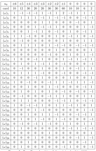
This is the result of a series of computer-assisted calculations, of independent interest and whose details will appear elsewhere [23], but for which I provide a fairly comprehensive summary in Appendix C. For the sake of example, we obtain for the first few values ofk,
p6 = θ7θ12−θ13−θ6θ12−θ21+ 2θ27θ1+ 2θ2θ1−θ4θ1+θ5θ1−θ6θ1+θ6θ7θ1−2θ7θ1−θ8θ1−θ26
+ θ6θ72−θ72−θ3+θ2θ6+θ5θ6+θ2θ7+θ4θ7−2θ6θ7+θ2θ8−θ6θ8−θ7θ8, (2.25) p7 = θ74+ 2θ1θ73−4θ37+θ12θ72−6θ1θ27+ 2θ2θ72+ 2θ5θ27−2θ6θ72+θ72−2θ31θ7−θ21θ7+ 4θ1θ7
+ 4θ1θ2θ7−θ3θ7+θ4θ7+ 2θ1θ5θ7−4θ5θ7+θ1θ6θ7+ 4θ6θ7−θ1θ8θ7−θ6θ8θ7
+ θ13+ 2θ21+θ22+θ52+θ1θ62+θ62+θ1θ82+θ1−θ1θ2−2θ1θ3−θ3+θ1θ4+θ4−2θ21θ5
+ 2θ2θ5−θ5+ 2θ21θ6+ 3θ1θ6−θ2θ6+θ4θ6−2θ5θ6+θ6−θ12θ8−θ1θ8+θ2θ8
− 2θ2θ7−θ8θ7+ 2θ7−θ4θ8−θ1θ6θ8−3θ1θ5 (2.26) p8 = θ8−θ14−θ6θ13+ 2θ72θ21+ 3θ2θ12−θ4θ21+θ5θ21+θ6θ21−θ7θ21−2θ7θ8θ21−2θ73θ1+θ62θ1
+ 3θ6θ72θ1−3θ3θ1+ 2θ4θ1−θ5θ1+ 2θ2θ6θ1+θ5θ6θ1+ 2θ6θ1+ 2θ2θ7θ1+θ4θ7θ1
+ 2θ6θ7θ1+ 5θ7θ1+θ72θ8θ1+θ2θ8θ1−2θ5θ8θ1−3θ7θ8θ1+θ8θ1−2θ74+θ6θ73+θ37
− 2θ52+θ26−θ2θ72+ 2θ4θ27−4θ5θ72+ 3θ27−θ28+θ2+θ3+θ2θ4−θ4−2θ2θ5
− 2θ3θ6+θ4θ6−θ5θ6+θ62θ7+θ2θ7−3θ3θ7+θ5θ7+ 2θ2θ6θ7+θ5θ6θ7+θ6θ7−2θ7
− θ2θ8−3θ3θ8+ 2θ4θ8−3θ5θ8+ 2θ6θ8+ 3θ2θ7θ8+ 2θ6θ7θ8+ 4θ7θ8,
− θ72θ1+ 2θ4θ5+ 2θ5−3θ5θ7θ1+θ38−θ22−4θ72θ8 (2.27) p9 = 2θ12θ37−2θ74−7θ1θ73−3θ6θ73+ 4θ37−2θ13θ27−θ21θ27+θ62θ27+θ28θ27+ 10θ1θ72+ 4θ1θ2θ72
− 2θ3θ72+θ4θ72+ 2θ1θ5θ72−5θ5θ72+ 2θ1θ6θ72+ 2θ6θ27+θ6θ8θ72−θ8θ72−2θ27+ 2θ13θ7+θ12θ7
+ θ22θ7+ 2θ1θ62θ7+ 6θ62θ7+θ1θ82θ7−2θ82θ7−θ1θ7−3θ1θ2θ7+ 5θ2θ7−4θ1θ3θ7+ 2θ3θ7
+ 2θ1θ4θ7−2θ21θ5θ7−6θ1θ5θ7+ 2θ2θ5θ7+ 5θ5θ7+θ21θ6θ7+ 5θ1θ6θ7+ 2θ2θ6θ7+ 3θ4θ6θ7
− 4θ5θ6θ7+ 4θ6θ7−2θ1θ8θ7+θ4θ8θ7−2θ5θ8θ7−2θ1θ6θ8θ7−θ6θ8θ7+θ8θ7−θ13+ 2θ36
+ 2θ42−θ25+ 2θ1θ26+θ2θ26+ 3θ62−θ1θ82+θ2θ82+θ5θ82+ 2θ1θ2+θ2+θ12θ3+θ1θ3−2θ2θ3
− θ1θ4−2θ2θ4−θ4+θ12θ5+ 2θ1θ5−2θ2θ5−3θ3θ5−θ21θ6+θ1θ6+θ1θ2θ6+ 4θ2θ6−2θ3θ6
+ θ1θ4θ6−θ4θ6−2θ1θ5θ6+θ5θ6+θ6−θ31θ8+ 2θ1θ2θ8−θ3θ8−2θ1θ4θ8+θ4θ8+θ1θ5θ8
− θ12θ6θ8+θ2θ6θ8−θ5θ6θ8−θ21+θ21θ4−4θ2θ27−θ4θ7. (2.28)
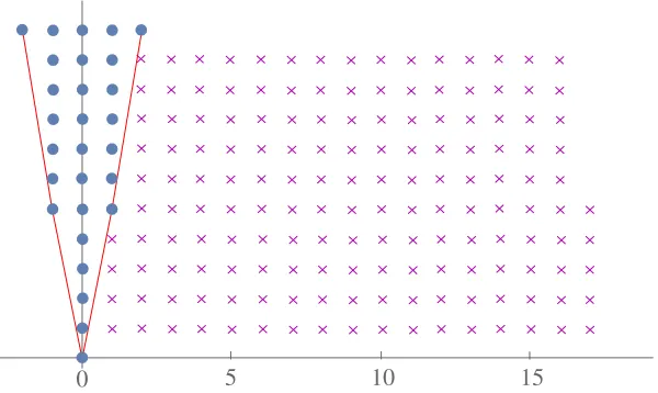
2.4.1. Genus, ramification points, and points at infinity. The curves Γu,ℵ have two obvious
in-volutions, coming from the Z2 ×Z2 symmetry (2.20) of the reduced characteristic polynomial
Ξg,red,
20 40 60 80 100 120 2
4 6 8
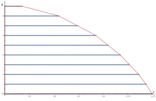
[image:16.612.148.461.70.274.2]x y
Figure 3. The Newton polygon of Ξ′′g,red (in red); blue spots depict monomials in Ξ′′
g,red with non-zero coefficients; the purple cross marks the vanishing of the
coefficient ofx101y3 on the boundary of the polygon.
This realises Γu,ℵ y
→Γ′u,ℵ→x Γ′′u,ℵ, where x=µ+µ−1,y=λ+ℵλ−1, as a branched fourfold cover of a curve Γ′′
u,ℵ,{Ξ′′g,red(y, x) = 0}, so that
Ξg,red(λ′, µ) =:µ120Ξ′′g,red
λ′+ ℵ
λ′, µ+
1
µ
(2.30)
We see from (2.20) and (C.2) that degyΞ′′g,red(y, x) = 9, degxΞ′′g,red= 120. The Newton polygon of Ξ′′
g,redis depicted in Figure 3. By way of example, some of the simplest coefficients on the boundary
are given by:
[y9]Ξ′′g,red = (x+ 1)3(x+ 2) −1 +x+x25, (2.31) nh
xdegx[yi]Ξ′′g,red i
Ξ′′g,redo8
i=0 = {1,−1,−1,−3u7−5,1,2,1,−2,1}. (2.32)
Let us now compute the genus of Γ′′u, Γ′u and Γu,ℵ.
Proposition 2.4. We have, for generic (u,ℵ)∈Bg,
g(Γ′′u) = 61, g(Γu′) = 128, g(Γu,ℵ) = 495. (2.33) Proof. Since Lemma 2.2 and Claim 2.3 determine the polynomial Ξ′′
g,redcompletely, the calculation
of the genus can be turned into an explicit calculation of discriminants of Ξ′′g,red; and because degyΞ′′g,red ≪ degxΞ′′g,red, it is much easier to start from the y-discriminant. This is computed to be
DiscryΞ′′g,red= (x+ 2)4∆1(x)∆2(x)2∆3(x)2 (2.34)
where deg ∆1 = 133, deg ∆2 = 215 and deg ∆3 = 392. Call rik, i= 1,2,3, k = 1, . . . ,deg ∆i the
roots of ∆i. We can verify directly by substitution into Ξ′′g,red that the roots x = r2k and x =rk3
correspond to images on thex-line of exactly one point with∂yΞ′′g = 0, which is always an ordinary
double point. Similarly, we get that the rootsx=−2 andx=rk1 correspond in all cases to degree 2 ramification points; there are four of them lying over x =−2. On the desingularised projective curve Γ′′
u, the nodes are resolved into pairs of unramified points; and Puiseux expansions of Ξ′′g,red
at infinity show that we have one extra point with degree 2 ramification abovex=∞ (see below). By Riemann–Hurwitz, this gives
g(Γ′′u) = 1−degyΞ′′g,red+1 2
X
P|dx(P)=0
ex(P) = 1−9 +
133 + 1 + 4
2 = 61. (2.35)
The genera of the branched double covers x : Γ′u → Γ′′u, y : Γu,ℵ → Γ′u follow from an elementary
Riemann–Hurwitz calculation.
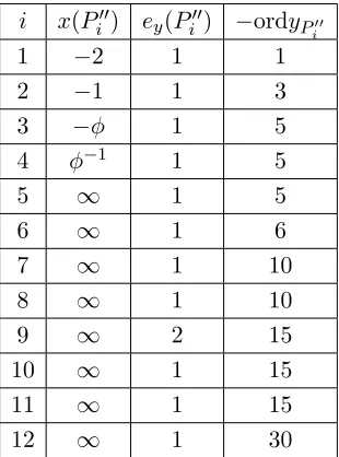
Remark 2.5. It can readily be deduced from (2.31) that the smooth completion Γ′′
u is obtained
topologically by adding 12 points at infinity Pi′′; their relevant properties are shown in Table 1. Their pre-images in Γ′u and Γu,ℵ will be labelled Pk′ andPj respectively,k= 1, . . . ,23 (notice that P′′
1 is a branch point ofx: Γ′u→Γ′′u),j= 1, . . . ,46.
i x(Pi′′) ey(Pi′′) −ordyP′′
i
1 −2 1 1
2 −1 1 3
3 −φ 1 5
4 φ−1 1 5
5 ∞ 1 5
6 ∞ 1 6
7 ∞ 1 10
8 ∞ 1 10
9 ∞ 2 15
10 ∞ 1 15
11 ∞ 1 15
[image:17.612.229.384.311.520.2]12 ∞ 1 30
Table 1. Points at infinity in Γ′′
u. I indicate the value of their x-projection, their
degree of ramification iny, and the order of the poles ofy in the second, third, and fourth column respectively. Here φ= √5+12 is the golden ratio.
2.5. Spectral vs parabolic vs cameral cover. The construction of Γu,ℵ as the non-trivial
irre-ducible component of the vanishing locus of (2.17)-(2.22) realises it as a “curve of eigenvalues”: it is a branched cover of the space of spectral parametersλ∈P1\ {0,∞}of the Lax matrixLd
x,y(λ);
the fibre over a λ-unramified point is given by the eigenvaluesµα ofLdx,y(λ) that are different from
1. By (2.22), each sheet µα is labeled by a non-trivial root α ∈∆∗, and there is an action of the
Weyl group W on Γu,ℵ given by the interchange of sheets corresponding to the Coxeter action of
W on the root space ∆.
Away from the ramification locus, this structure can be understood as follows. Let
Gred={g∈ G|dimCCG(g) = rank G= 8}
be the Zariski open set of regular elements of G; I’ll similarly append a superscript Tred for the
regular elements ofT. Then the projection
π :G/T × Tred → Gred
(gT, t) → Adgt (2.36)
is a principalW-bundle onGred, the fibre over a regular elementg′ beingN
T/T ≃ W. We can pull
this back via Ldx,y to aW-bundle
Θx,y ,Ldx,y∗(G/T × Tred)
over P1\D, where D =Ld x,y−
1
(G \ Gred). This is a regular W-cover and each weight ω ∈ Λ w(G)
determines a subcover Θω
x,y ≃Θx,y/Wω, where we quotient by the action of the stabiliser of ω by
deck transformations. Write Θx,y and Θωx,y for the pull-back to C⋆ ≃P1\ {0,∞} of the closure of
(2.36) in G/T × T → G. As in [37], we call Θx,y (resp. Θωx,y) the cameral (resp. the ω-parabolic)
cover associated toLbx,y.
Notice that when ω =ω7 =α0 is the highest weight of the adjoint representation, i.e. the highest
(affine) root α0,W/Wα0 is set-theoretically the root system ofg, minus the set of zero roots; the
residual W action is just the restriction to ∆ of the Coxeter action on h∗. In particular, we have that Θω
x,y is a degree|W/Wα0|=|Weyl(e8)/Weyl(e7)|= 6967296002903040 = 240 branched cover ofP1, with
sheets labelled by non-zero rootsα ∈∆∗.
Proposition 2.6. There is a birational map ι: Γu,ℵ99KΘω7x,y given by an isomorphism ι: Γu,ℵ\ {dµ= 0} →∼ Θω7x,y
(λ, µα(λ)) → (λ, α) (2.37)
away from the ramification locus of the λ-projection.
Proof. The proof is nearly verbatim the same as that of [86, Thm. 13].
From the proposition, we learn that a possible source of ramificationλ: Γu,ℵ→P1 comes from the
spectral values λsuch that Lbx,y(λ) is an irregular element of G; and from (2.22), we see that this
happens if and only if α(l) = 0 for some α∈∆.
Proposition 2.7. For generic (u,ℵ), there are exactly 18 values of λ, b±i ,λ(Q±
i ), i= 1, . . . ,9, (2.38) such that Lbx,y(λ) is irregular, i.e. α(logLbx,y(λ)) = 0 for some α ∈ ∆. Furthermore, α ∈Π is a simple root in each of these cases.
Proof. To see this, look at the base curve Γ′′u. It is obvious that Ξg,red has only double zeroes at x= 2, since Ξg has only double zeroes atµ= 1 as roots come in (positive/negative) pairs in (2.22). For each of the nine points
{Q′′i}9i=1 ,x−1(2)⊂Γ′′u,
we compute from Lemma 2.2 and Claim 2.3 that
ex(Q′′i) = 28 (2.39)
for all i. Calling αi ∈∆+ the positive root such thatαi·l(λ(Qi)) = 0, we see from (2.22) that ex(Q′′i) = card
β ∈∆+|β−αi∈∆+ . (2.40)
It can be immediately verified that the right hand side is less than or equal to 28, with equality iff
αi is simple. It is also clear that there are no other points of ramification in the affine part of the
curve4 ; indeed, from Table 1, we have that ex(∞) = 120−12 = 108, and from (2.33) we see that
60 =g(Γ′′u)−1 =−degxΞ′′g,red+1 2
X
dx(P)=0
ex(P) =−120 +
9×28 + 108
2 . (2.41)
As the covering mapx: Γ′u→Γ′′u is ramified atx= 2, and y: Γu,ℵ→Γ′u is generically unramified
therein for genericℵ, we have two preimagesQi,± on Γu,ℵ for each Q′′i ∈Γ′′u.
3. Action-angle variables and the preferred Prym–Tyurin
Since (2.14) are a complete set of Hamiltonians in involution on the leaves of the foliation of Pb by level sets of ℵ, the compact fibres of the map (u,ℵ) : P →b C9 are isomorphic to a rank(g) =
8-dimensional torus by the (holomorphic) Liouville–Arnold–Moser theorem. A central feature of integrable systems of the form (2.16) is an algebraic characterisation of their Liouville–Arnold dynamics, the torus in question being an Abelian sub-variety of the Jacobian of Γu,ℵ.
I determine in this section the action-angle integration explicitly for theEb8 relativistic Toda chain,
which results in endowingSg with extra data [38, 76], as per the following
Definition 3.1. We callDubrovin–Krichever data a n-tuple (F,B,E1,E2,D,Λ,ΛL), with
• π :F →B a family of (smooth, proper) curves over an n-dimensional varietyB;
• D a smooth normal crossing divisor intersecting the fibres of π transversally;
• meromorphic sections Ei ∈H0(F, ωF/B(logD)) of the relative canonical sheaf having log-arithmic poles along D;
• (ΛL,Λ) a locally-constant choice of a marked subring Λ of the first homology of the fibres, and a Lagrangian sublattice ΛL thereof.
4In principle, from (2.22), this would be the case ifα(l(λ)) =β(l(λ)) forα−β /∈∆, leading to a double zero at
Definition 3.1 isolates the extra data attached to spectral curves that were identified in [38, 76] (see also [39, 77]) to provide the basic ingredients for the construction of a Frobenius manifold structure onBand a dispersionless integrable dynamics on its loop space given by the Whitham deformation of the isospectral flows (2.16); the logarithm of those τ-functions respects the type of constraints that arise in theory with eight global supersymmetries (rigid special K¨ahler geometry). These will be key aspects of the story to be discussed in Sections 4 and 5; in the language of [38], when the pull-back of E1 to the fibres of the family is exact, the associated potential is the superpotential of the
Frobenius manifold, andE2 its associated primitive differential. Now, Claim 2.3 and Definition 2.1
gave us F = Sg, B = Bg already. We’ll see, following [77], how the remaining ingredients are determined by the Hamiltonian dynamics of (2.16): this will culminate with the content of Theorem 3.6. I wish to add from the outset that the process leading up to Theorem 3.6 relies on both common lore and results in the literature that are established and known to the cognoscenti
at least for the non-relativistic limit; the gist of this section is to unify several of these scattered ideas and adapt them to the setting at hand. For the sake of completeness, I strived to provide precise pointers to places in the literature where similar arguments have been employed.
3.1. Algebraic action-angle integration. From now until the end of this section, I will be sitting at a generic point (x, y) ∈ Pb, and correspondingly, smooth moduli point (u,ℵ) ∈ Bg. As
is the case for the ordinary periodic Toda chain withN particles, and for initial data specified by (u,ℵ), the compact orbits of (2.16) are geometrically encoded into a linear flow on the Jacobian variety Pic(0)(Γu,ℵ) [2, 60, 75, 117]; I recall here why this is the case. The eigenvalue problem5 at
time-t,
d
Lx,y(λ)Ψx,y=µΨx,y (3.1)
withx=x(~t),y=y(~t), endows the spectral curve with an eigenvector line bundleLx,y→Γu,ℵ and
a section Ψ : Γu,ℵ→ Lx,y given as follows. We have an eigenspace morphism
Ex,y : Γu,ℵ→Pdimg−1 =P247 (3.2)
that, away from ramification points of theλ: Γu,ℵ→P1projection, assigns to a point (λ, µ)∈Γu,ℵ
the (time-dependent) eigenline of (3.1) with eigenvalueµ; this in fact extends to a locally free rank one sheaf on the whole of Γu,ℵ [7, Ch. 5, II Proposition on p.131]. We write
Lx,y ,Ex,y∗ OP247(1)∈Pic(Γu,ℵ) (3.3)
for the pullback of the hyperplane bundle on Pdimg−1 via the eigenline map E
x,y, and fix
(non-canonically) a section of the latter by
Ψj(λ, µi(λ)) =
∆j1
d
Lx,y(λ)−µi(λ)
∆11
d
Lx,y(λ)−µi(λ)
, (3.4)
5For ease of notation, and since we’ve fixedρ=gin the previous section, I am dropping here any reference to the
representationρof the Lax operator.
where µi(λ) = exp(αi(l(λ)) (cfr. (2.22)) and we denoted by ∆ij(M) the (i, j)th minor of a matrix M. Astand x(t), y(t) vary, so willLx(t),y(t), and
Bx,y(t),Lx,y(t)⊗ L∗x,y(0)∈Pic(0)(Γu,ℵ)≃
H1(Γu,ℵ,O) H2(Γ
u,ℵ,Z)
(3.5)
is a time-dependent degree zero line bundle on Γu,ℵ.
The flows (2.16) thus determine a flowt→ Bx(t),y(t)in the Jacobian of Γu,ℵ, which is actuallylinear
in Cartesian coordinates for the torus Pic(0)(Γu,ℵ). Indeed, let {ωk}k be a basis for the C-vector
space of holomorphic differentials on Γu,ℵ,Ch{ωk}ki=H1(Γu,ℵ,O), and let ψ: SymgΓu,ℵ → Pic(0)(Γu,ℵ)
(γ1+· · ·+γg) → g X
i=1
A(pi) (3.6)
be the surjective, degree one morphism from thegth-symmetric power of Γ
u,ℵto its Jacobian, given
by taking the Abel sums ofg unordered points on Γu,ℵ; here
A: Γu,ℵ → Pic(0)(Γu,ℵ)
γ →
Z γ
dω1, . . . , Z γ
dωg
(3.7)
denotes the Abel map for some fixed choice of base point. Writing
Symg ∋γ(t) = (γ1(t), . . . , γg(t)) =ψ−1(Bx(t),y(t))
for the inverse of Bx(t),y(t), which is unique for generic time t by Jacobi’s theorem, we have that
[117, Thm. 4]
Ωik , ∂ ∂ti
g X
j=1 Z γj(t)
ωk =
X
p∈λ−1(0)∪λ−1(∞)
Resp h
ωkPi(Ldx,y(λ)) i
∀ k= 1, . . . , g (3.8)
The left hand side is the derivative of the flow on the Jacobian (its angular frequencies) in the chart on Pic(0)(Γu,ℵ) determined by the linear coordinatesH1(Γu,ℵ,O) w.r.t the chosen basis{ωk}k. The
right hand side shows that this is independent of time, and hence the flow is linear in these co-ordinates, since ωk and Pi(Ldx,y(λ))) are: the former since it only feels the dynamical phase space
variables {xi, yi}8i=0 inLdx,y(λ) via Γu,ℵ, itself an integral of motion, and the latter by (2.16).
3.2. The Kanev–McDaniel–Smolinsky correspondence. The story above is common to a large variety of systems (the Zakharov–Shabat systems with spectral-parameter-dependent Lax pairs), and the Ec8 relativistic Toda fits entirely into this scheme. In particular, in the better
known examples of the periodic relativistic and non-relativistic Toda chain with N-particles (i.e.
g = slN;ρ = in (2.16)), where the spectral curves have genus g =N −1, the action-angle map
{xi, yi} →(Γu,ℵ,Lx,y) gives a family of rankg=N−1 commuting flows on theirN−1-dimensional
Jacobian. A question that does not arise in these ordinary examples, however, is the following: in our case, we have way more angles than we have actions, as the genus of the spectral curve is
much higher than the rank ofg=e8. Indeed, the Jacobian is 495-complex dimensional in our case
by (2.33); but the (compact) orbits of (2.33) only span an 8-dimensional Abelian subvariety of the Jacobian.
How do we single out this subvariety geometrically? In the non-relativistic case, pinning down the dynamical subtorus from the geometry of the spectral curve has been the subject of intense study since the early studies of Adler and van Moerbeke [2] for g = bn,cn,dn,g2, and the fundamental
works of Kanev [68], Donagi [37] and McDaniel–Smolinsky [87, 88] in greater generality. We now work out how these ideas can be applied to our case as well.
Recall from Proposition 2.6 that we have aW-action on Γu,ℵby deck transformations given by
φ:W ×Γu,ℵ → Γu,ℵ
(w, λ, µα(λ)) → (λ, µw(α)(λ)) (3.9)
which is just the residual action of the vertical transformations on the cameral cover. Write φw , φ(w,−) ∈ Aut(Γu,ℵ) for the automorphism corresponding to w ∈ W. Extending by linearity, φw induces an action on Div(Γu,ℵ) which obviously descends to give actions on the Picard group
Pic(Γu,ℵ), the Jacobian Pic(0)(Γu,ℵ) ≃ Jac(Γu,ℵ) (since φw is compatible with degree and linear
equivalence), and theC-space of holomorphic 1-formsH1(Γu,ℵ,O). At the divisorial level we have
furthermore an action of the group ring
ϕ:Z[W]×Div(Γu,ℵ) → Div(Γu,ℵ),
X
i aiwi,
X
j
bj(λj, µα(λj))
→ X
i,j
aibj(λj, µwi(α)(λj)). (3.10)
Recall from Proposition 2.6 that, since the group of deck transformations of the cover Γu,ℵ\{dµ= 0}
is isomorphic to the Coxeter action of W on the root space ∆≃ W/Wα0, the map (3.10) factors
through the coset projection mapW →∆, i.e.
ϕ(w,−) =|Wα0| X
α∈∆
˜
aαwα, (3.11)
for some {˜aα ∈ Z}α∈∆. Restrict now to elements ϕ(w,−) ∈ Z[W] such that ϕ(w,−) : Z[W] → Z[Aut(Γu,ℵ)] is a ring homomorphism. Then the action (3.10) is the pull-back of an action of the
maximal subgroup of Z[∆] which respects the product structure induced from Z[W]: this is the Hecke ring H(W,Wα0)≃ Z[Wα0\W/Wα0]≃Z[∆]Wα0. Its additive structure is given by the free Z-module structure on the space of double cosets of W by Wα0, and its product is defined as the
push-forward6 of the product on Z[W]. In practical terms, this forces the integers aα in the sum
over roots in ∆∗ (i.e. right cosets ofW/Wα0) to be constant over left cosetsWα0\W in (3.11).
The Weyl-symmetry action is the key to single out the Liouville-Arnold algebraic torus that is home to the flows (2.16). We first start from the following
6That is, the image under the double-quotient projection of the product of the pullback functions onW, which is
well-defined on the double quotient even whenWα0 is not normal, as in our case.
Definition 3.2. Let D ∈ Div(Γ×Γ) be a self-correspondence of a smooth projective irreducible curve Γ and let C ∈End(Γ) be the map
C : Jac(Γ) → Jac(Γ)
γ → (p2)∗(p∗1(γ)· D), (3.12) where pi denotes the projection to the ith factor in Γ×Γ. The Abelian subvariety
PTC(Γ),(id− C) Jac(Γ) (3.13)
is called a Prym–Tyurin variety iff
(id− C)(id− C −qC) = 0 (3.14)
for qC ∈Z, qC≥2.
By (3.14), the tangent fibre at the identityTe(Jac(Γ)) splits into eigenspacesTe(Jac(Γ)) =tPT⊕t∨PT
of C with eigenvalues 1 and 1−qC. BecauseqC ∈Z, these exponentiate to subtoriTPT = exptPT,
TPT∨ = expt∨PT, with TPT = PTC(Γ), such that Jac(Γ) = TPT× TPT∨ . In particular, in terms of
the linear spaces VPT≃TgPT,VPT∨ ≃TgPT∨ which are the universal covers of the two factor tori, we
have
PTC(Γ)≃VPT/ΛPT (3.15)
where ΛPT = H1(Γ,Z)∩VPT. Furthermore [68], there is a natural principal polarisation Ξ on
PTC(Γ) given by the restriction of the Riemann form Θ onH1(Γ,O)≃VPT⊕VPT∨ toVPT; we have
Θ = qCΞ, with Ξ unimodular on ΛPT. In particular, id− C acts as a projector on the space of
1-holomorphic differentials, and, dually, 1-homology cycles on Γ, such that
• the projection selects a symplectic vector space VPT ⊂H1(Γ,O) and dual subring ΛPT ∈ H1(Γ,Z); 1-forms inVPT have zero periods on cycles in Λ∨PT;
• bases{ω1, . . . , ωdimVPT},{(Ai, Bi)}dimVPTi=1 can be chosen such that the corresponding matrix
minors of the period matrix of Γ satisfy Z
Aj
ωi=qCδij, Z
Bj
ωi =τij (3.16)
with τij non-degenerate positive definite.
There is a canonical element ofH(W,Wα0) which has particular importance for us, and which will
eventually act as a projector on a distinguished Prym–Turin subvariety of Jac(Γu,ℵ). This is the
Kanev–McDaniel–Smolinsky self-correspondence7[68, 87, 88]
Pg, X
w∈W/Wα0
w−1(α0), α0
w. (3.17)
I summarise here some of its key properties, some of which are easily verifiable from the definition (3.17), with others having been worked out in meticulous detail in [87, Sec. 3–5]. Some further
7This has also been considered in the gauge theory literature, implicitly in [64, 85] and more diffusely in [82].
explicit results that are relevant to our case, but that did not fit in the discussion of [87], are presented below.
Proposition 3.1. In the root space (h∗,h,i) consider the hyperplanes
Hi={β ∈h∗| hβ, α0 =ii}. (3.18) Then, set-theoretically,Wα0\W/Wα0 ≃ {δi ,Hi∩∆}2i=−2. LettingW
π1
−→ W/Wα0 −→ Wπ2 α0\W/Wα0 be the projection to the double coset space and {si}2i=−2=π2(∆), we furthermore have
Pg=π∗2
X
δi∈Wα0\W/Wα0
isi∈H(W,Wα0)
. (3.19)
Proof. The fact that Pg ∈ Z[∆]Wα0 = H(W,W
α0) follows immediately from its definition in
(3.17) and the constancy ofw−1(α
0), α0on left cosets. The rest of the proof follows from explicit
identification of the elements ofH(W,Wα0) in terms of the hyperplanes of (3.18), and evaluation of
(3.17) on them. The proof is somewhat lengthy and the reader may find the details in Appendix A.
Corollary 3.2. Pg satisfies the quadratic equation in H(W,Wα0) with integral roots
Pg2=qgPg (3.20)
with
qg= 60. (3.21)
In particular, the correspondence C = 1−Pg defines a Prym–Tyurin variety PT1−Pg(Γu,ℵ) ⊂ Jac(Γu,ℵ).
Proof. This is a straightforward calculation from Eq. (3.19).
In the following, I will simply write PT(Γu,ℵ), dropping the 1−Pgsubscript which will be implicitly assumed.
The main statement about PT(Γu,ℵ) is the subject of the next Theorem. Note that this bears a large
intellectual debt to previous work in [68, 88]; the modest contribution of this paper is a combination of the results of this and the previous Section with [68, 88] to prove that the Liouville–Arnold torus (the image of the flows (2.16) on the Jacobian) is indeed isomorphic to the full Kanev–McDaniel– Smolinsky Prym–Tyurin, rather than being just a closed subvariety thereof.
Theorem 3.3. The flows (2.16), (3.8) of the Ec8 relativistic Toda chain linearise on the Prym– Tyurin variety PT(Γu,ℵ) and they fill it for generic initial data (u,ℵ).
Proof. The linearisation of the flows on PT(Γu,ℵ) amounts to say that X
p∈λ−1{0,∞}
Resp h
ωPi(L\x,y(λ)) i
6
= 0 ⇒ Pg∗ω=ω (3.22)
in (3.8). This is essentially the content of [68, Theorem 8.5] and especially [88, Theorem 29], to which the reader is referred. The latter paper greatly relaxes an assumption on the spectral dependence ofLbx,y(λ) [68, Condition 8.4] which renders incompatible [68, Theorem 8.5] with (2.12);
this restriction is entirely lifted in [88, Theorem 29], where the fact that (2.12) depends rationally on λis sufficient for our purposes. While [68, 88] deal with the non-relativistic counterpart of the system (2.16), it is easy to convince oneself that replacing their algebraic setting with the Lie-group arena we are playing in in this paper amounts to a purely notational redefinition of g toG in the arguments leading up to [88, Theorem 29].
Since the first part of the statement has been settled in [88], I now move on to prove that the Prym–Tyurin is the Liouville–Arnold torus. Denoting φ(i)t :P →b Pb be the time-t flow of (2.16), and for fixed (x, y)∈Pb, the above proves that
φ(1)t1 · · · · ·φ(8)t8 :P1× · · · ×P1 → Pb
(x, y) → (x(~t), y(~t)) (3.23) surjects to an eight-dimensional subtorus of PT(Γu,ℵ). To see the resulting torus is the Prym–
Tyurin, we use the dimension formula of [87, Theorem 17]. LetC⋆,P1\{b±i }9i=1,M:π1(C⋆)→ W
be the Galois map of the spectral cover Γu,ℵ, and for P ∈ Γu,ℵ write S(P) for the stabiliser of P
in the group of deck transformations of Γu,ℵ, and h∗P for the fixed point eigenspace of S(P) ⊂ W.
Then [87, Theorem 17]
dimCPT(Γu,ℵ) =
1 2
X
λ(p)|dµ(p)=0
8−dimCh∗p−8 +h,C[W/M(π1(P1⋆))]
(3.24)
where one representativepis chosen in each fibre ofλ: Γu,ℵ→P1. In our case,M(π1(P1⋆)) =W by
Proposition 2.6 and the fact that theα0-parabolic cover is irreducible (hence a connected covering
space ofP1), so the last term vanishes. Then
dimCPT(Γu,ℵ) =
1 2
X
i=1,...9,j=±
8−dimCh∗Qi,j
+1 2
X
j=±
8−dimCh∗Q∞,j
−8 (3.25)
where Qi,j=± are the ramification points of the λ-projection as in Proposition 2.7. Since αk(i)· µ(Qi,±) = 0 for some permutationk:{1, . . . ,8} → {1, . . . ,8}, the deck transformations in S(Qi,±)
are simple reflections that stabilise the hyperplane orthogonal to the rootαk(i), so that dimCh∗Qi,j =
7. As far asQ∞,±are concerned, the deck transformation associated to a simple loop around them
corresponds to the product of the Coxeter element ofW times a simple root, as this is the lift under the projection to the base curve of a loop around all branch points on the affine part of the curve8. Then dimCh∗Q∞,j = 1, dimCPT(Γu,ℵ) = 8, and the flows (3.23) surject on the latter.
An explicit construction of Kanev’s Prym–Tyurin PT(Γu,ℵ), after [85, Section 3], can be given as
follows. With reference to Figure 4, let γ±i be a simple counterclockwise loop around the branch
8The root in question is the one that is repeated in the sequence{k(i)}9
i=1. There could be more of them in principle, but this would be in contrast withM(π1(P1⋆)) =W; equivalently,a posteriori, this would lead to dimCPT(Γu,ℵ)<8, contradicting the independence of the flows (2.16), which in turn is a consequence of the algebraic independence of the fundamental charactersθiinR(G).

![Table 4. Degree and genera of minimal spectral curve (putative) mirrors of X�g,¯i forthe exceptional series EFG; for simplicity I only indicate the genus for the originalchoice of marked node ¯i in [43, Table I].](https://thumb-us.123doks.com/thumbv2/123dok_us/7734220.163573/70.612.124.489.72.169/minimal-spectral-putative-mirrors-exceptional-simplicity-indicate-originalchoice.webp)