White Rose Research Online URL for this paper:
http://eprints.whiterose.ac.uk/112670/
Version: Accepted Version
Article:
Cai, J., Liu, W., Zong, R. et al. (1 more author) (2017) An Expanding and Shift Scheme for
Constructing Fourth-Order Difference Co-Arrays. IEEE Signal Processing Letters. ISSN
1070-9908
https://doi.org/10.1109/LSP.2017.2664500
© 2016 IEEE. Personal use of this material is permitted. Permission from IEEE must be
obtained for all other users, including reprinting/ republishing this material for advertising or
promotional purposes, creating new collective works for resale or redistribution to servers
or lists, or reuse of any copyrighted components of this work in other works. Reproduced
in accordance with the publisher's self-archiving policy.
[email protected] https://eprints.whiterose.ac.uk/
Reuse
Unless indicated otherwise, fulltext items are protected by copyright with all rights reserved. The copyright exception in section 29 of the Copyright, Designs and Patents Act 1988 allows the making of a single copy solely for the purpose of non-commercial research or private study within the limits of fair dealing. The publisher or other rights-holder may allow further reproduction and re-use of this version - refer to the White Rose Research Online record for this item. Where records identify the publisher as the copyright holder, users can verify any specific terms of use on the publisher’s website.
Takedown
If you consider content in White Rose Research Online to be in breach of UK law, please notify us by
An Expanding and Shift Scheme for Constructing
Fourth-Order Difference Co-Arrays
Jingjing Cai, Wei Liu, Ru Zong, and Qing Shen
Abstract—An expanding and shift (EAS) scheme for efficient fourth-order difference co-array construction is proposed. It consists of two sparse sub-arrays, where one of them is modified and shifted according to the analysis provided. The number of consecutive lags of the proposed structure at the fourth order is consistently larger than two previously proposed methods. Two effective construction examples are provided with the second sparse sub-array chosen to be a two-level nested array, as such a choice can increase the number of consecutive lags further. Simulations are performed to show the improved performance by the proposed method in comparison with existing structures.
Index Terms—Sparse arrays, fourth-order difference co-array, second-order difference co-array, cumulant.
I. INTRODUCTION
Recently, the sparse array concept combined with co-array equivalence has attracted significant interest in the community [1], [2], and two representative examples are the co-prime arrays [3]–[5], and the nested arrays [6], [7]. Sparse arrays can form a larger aperture size given the same number of antennas and more importantly provide much more degrees of freedom (DOFs) than traditional uniform arrays. Many methods have been proposed for underdetermined DOA estimation based on such arrays, such as the spatial smoothing-based subspace methods [8], [9], or compressive sensing (CS)-based methods [4], [10]–[13].
So far the majority of work for virtual array generation is based on the second-order statistics (SOS). However, it is possible to exploit the fourth-order statistics (FOS) to generate even more DOFs, such as the cumulant-based DOA estimation methods studied in [14]–[20] and the method based on quasi-stationary signals [21], [22]. Therefore, how to construct a sparse array with maximum fourth-order virtual array sensors has become a very important problem. In [22], [23], the existing nested arrays and co-prime arrays were extended for effective fourth-order virtual array generation by adding to the structure a third uniform linear array. It was shown that in
Copyright (c) 2015 IEEE. Personal use of this material is permitted. However, permission to use this material for any other purposes must be obtained from the IEEE by sending a request to [email protected]. This work was partially supported by the National Natural Science Foun-dation of China (61405150 and 61628101).
Jingjing Cai and Ru Zong are with the Department of Elec-tronic and Engineering, Xidian University, Xi’an, 710071, China (e-mail:
{jjcai,zongru}@mail.xidian.edu.cn). Jingjing Cai is also a visiting researcher at the Department of Electronic and Electrical Engineering, University of Sheffield, Sheffield, S1 3JD, UK.
Wei Liu is with the Department of Electronic and Electrical Engineering, University of Sheffield, Sheffield, S1 3JD, UK (e-mail: [email protected]). Qing Shen is with the School of Information and Electronics, Beijing Insti-tute of Technology, Beijing, 100081, China (e-mail: [email protected]).
this way, the number of consecutive virtual sensor lags can be increased significantly.
In this work, by analysing the generated fourth-order dif-ference lags, we can consider them as the sum of two second-order difference lags with the same range. Based on this observation, we propose a new sparse array construction scheme aiming to maximize the consecutive lags in the fourth order virtual co-array.
We start from two separate sparse sub-arrays, and each of them is configured at the second-order difference co-array (SODCA) level, such as the existing co-prime arrays or nested arrays. Then one of them is expanded uniformly by increasing the adjacent physical sensor spacing according to the number of second-order consecutive virtual array sensors of the other sparse sub-array. The last step is shifting the newly expanded array to a new position so that the number of fourth-order consecutive virtual array sensors is further increased and the first sensor of the expanded sub-array coincides with one of the physical sensors of the other sub-array. Due to the coincidence, one of the two physical sensors can be removed without affecting the resultant fourth-order DOFs in the consecutive range. It is also shown that if the second sub-array is a two-level nested array, the fourth-order consecutive virtual sensor range can be further increased. Compared with the fourth-order difference co-arrays (FODCAs) proposed in [22], [23], a higher number of consecutive lags is achieved by the proposed scheme.
This paper is organized as follows. The cumulant-based FODCAs are analyzed in Sec. II, and the proposed con-struction is introduced in detail in Sec. III. A comparison of the different fourth-order construction schemes is performed in Sec. IV. Simulation results are provided in Sec. V and conclusion drawn in Sec. VI.
II. CUMULANT-BASEDFOURTH-ORDERDIFFERENCE
CO-ARRAY
Suppose there are K far-field independent non-Gaussian narrowband signals sk(t)(k = 1, . . . , K) impinging on a
sparse linear array (SLA) of M sensors. Denote the unit spacing by d, which is equal to half wavelength λ/2. Then, positions of the SLA sensors can be expressed as
P ={p1·d, p2·d, . . . , pm·d, . . . , pM·d}. (1)
With the angle of arrival of the kth source being θk, the
observed signalxm(t)at themth sensor is given by
xm(t) = K
∑
k=1
wherenm(t)is the additive Gaussian noise of themth sensor,
and it is independent of the signals. Suppose 1 ≤i, j, u, v≤
M and {i, j, u, v} ∈ Z. The fourth-order cumulant value C(i,−j, u,−v) of the ith, jth, uth and vth sensor observed signals can be expressed as [14]
C(i,−j, u,−v) =cum[xi(t), x∗j(t), xu(t), x∗v(t)]
=
K
∑
k=1
exp[−j2π(pi−pj+pu−pv)dcosθk/λ]·
cum(x1(t), x∗
1(t), x1(t), x∗1(t))
(3)
where()∗ denotes complex conjugate, andcum()denotes the fourth-order cumulant operation. The fourth-order difference co-array not only has a much larger number of virtual sensors than the physical SLA, but also removes the Gaussian noise components, which will help improving the DOA estimation result further.
The fourth-order difference lag (pi−pj+pu−pv)
corre-sponding to the new virtual sensors can be written as
pi−pj+pu−pv= (pi−pj) + (pu−pv) (4)
Clearly, this fourth-order difference lag expression can be seen as two second-order difference lags added together. As a result, we could construct the FODCA by two separate SODCAs with different ranges. Although this will not be optimal, it could provide an effective solution for FODCA construction, as shown later.
III. PROPOSEDEXPANDING ANDSHIFT(EAS) SCHEME FORCONSTRUCTINGFODCAS
A. The EAS Scheme
We start from two separate sparse sub-arrays which are configured for SODCA generation. They can be different types of sparse arrays and have different number of physical sensors. Assume the first sub-array containsM physical sensors, while the second one contains N sensors. Their array position settings are defined as
P ={p1·d, p2·d, . . . , pm·d, . . . , pM ·d}
Q={q1·d, q2·d, . . . , qn·d, . . . , qN ·d}
(5)
wherepm·dandpn·d,m= 1,2, . . . , M,n= 1,2, . . . , N, are
the physical sensor positions of the two sub-arrays. We further assume that the number of consecutive SODCA sensors for the first sub-array P is CM, while it isCN for Q.
Based on the two sparse arrays, we can generate the fourth-order difference lags using the expression(pi−pj)+(pu−pv)
in (4), where one choice is that the lags(pi−pj)come from
the second-order co-array of P, while (pu−pv) from that
of Q. When adding these two together, the segment of CM
consecutive virtual sensors fromPare then shifted one by one by the second-order virtual co-array sensors of Q, and there are at least CN copies of the same CM consecutive points
from P, which are then added together to form the FODCA. To make sure there are no overlaps or gaps among the CN
copies of the continuous segment of length CM so that the
maximum number of consecutive fourth-order virtual sensors are achieved, we can increase the unit spacing of the sub-array
QtoCM·d. As a result, the second sparse array is changed
to
˜
Q={q1, q2, . . . , qn, . . . , qN} ·CMd , (6)
and the number of consecutive fourth-order virtual co-array sensors isCL=CMCN.
Note that the CL consecutive lags in the fourth-order
co-array is independent of the relative positions of the two sparse arrays P and Q˜, since any shift will be canceled by the operation of (pi −pj) and (pu −pv). As a result, we can
shift the starting position of the second array Q˜ by∆s·dso that one of the physical sensors of the second sparse array will be co-located with one of the physical sensors of the first array, i.e. qnCM = pm for a specific pair of (m, n). Then,
one of the co-located sensors can be removed and the total number of physical sensors will be L = M +N −1 with the same number of consecutive fourth-order co-array sensors CL. To have a larger aperture, we can choose q1CM =pm,
i.e. the first sensor of the second array will coincide with one arbitrary sensor of the first array. Without loss of generality, we remove the first sensor of the second array Q˜. Then, the pair of sparse sub-arrays becomes
P ={p1·d, p2·d, . . . , pm·d, . . . , pM ·d}
ˆ
Q={q2, . . . , qn, . . . , qN} ·CMd ,
(7)
Interestingly, as we will show in the next part, this choice of shift will have the advantage of generating additional consecutive lags of 2(pm−p1) if the second sparse array
is chosen to be a two-level nested array (referred to as EAS-NA in the following). Under this condition, if the first array is further chosen to be either a nested array or a co-prime array, we can have q1CM = pM, so that the total
number of consecutive fourth-order co-array sensors becomes CL = CMCN + 2(pM −p1) for the EAS-NA scheme.The
physical array aperture of the proposed construction scheme is(qNCM−p1)dfor the general case ofq1CM =pm.
B. The EAS-NA Scheme
In this part, we consider the EAS-NA scheme, as it will increase the fourth-order consecutive lags further.
For a nested array, we have the interesting property of qN −q1 = CN2−1, where CN−2 1 is the maximum number
of positive consecutive second-order lags. For such an EAS-NA construction, the range of the positive consecutive fourth-order lags is from 1 to (qN −q1)CM + CM−2 1, and the
last segment of CM consecutive fourth-order lags is from
(qN −q1)CM − CM2−1 to (qN −q1)CM + CM−2 1, centered
at(qN −q1)CM. With q1CM =pM as suggested in the last
subsection, this center becomesqNCM−pM
Note that the last sensor ofQ˜ isqNCM. When calculating
the fourth-order difference lag(pi−pj) + (pu−pv),pi andpj
can be chosen from the first arrayP, while pu=qNCM and
pv =p1. For such a choice,(pi−pj)will general a segment
of consecutive lags from−CM−1 2 to
CM−1
2 , so that(pi−pj)+
(pu−pv)in total will generate a segment of consecutive lags
fromqNCM−p1−CM2−1 toqNCM −p1+CM−2 1, centered
Now we have two segments of consecutive lags of length CM, one centered at qNCM −pM and one at qNCM −p1,
where the second one is pM −p1 away from the first one. If
pM −p1≤(CM−1), then the consecutive fourth-order lags
will be increased fromCMCN toCMCN+2(pM−p1), where
the multiplication by2is due to considering both the negative and the positive consecutive lags. Since the condition pM −
p1≤(CM−1)is satisfied for most sparse arrays designed for
maximizing the continuous second-order difference co-array lags, such as the co-prime arrays and nested arrays, we can shift the second sparse array so that its first sensor will be co-located with the last sensor of the first array.
C. Examples of the EAS-NA Scheme
Here, we give two examples for the EAS-NA scheme. One takes two nested arrays as its two sparse sub-arrays, referred to as the EAS-NA-NA array; the other one use the co-prime array as its first sparse sub-array and the nested array as the second sparse sub-array, referred to as the EAS-NA-CPA array. First we consider the EAS-NA-NA case. The first nested array contains M1 and M2 sensors in its two sub-arrays,
separately, and the second nested array contains N1 andN2
sensors. The total number of sensors isL=M1+M2+N1+
N2−1. The consecutive second-order co-array sensor number of these two nested arrays is CM = 2M1M2+ 2M2−1and
CN = 2N1N2+ 2N2−1, respectively. The first sensor of the
first nested array is1and the last sensor ispM =M1M2+M2.
Then, the total number of consecutive fourth-order difference co-array lags is CL= (2M1M2+ 2M2−1)(2N1N2+ 2N2−
1) + 2(M1M2+M2−1).
As an example, for M1=N1= 2 andN1=N2= 2, we have CM = CN = 11and CL = 131. The resultant sensor
locations are P ={1,2,3,6} ·dandQˆ ={17,28,61} ·d. Now for the EAS-NA-CPA case, assume the co-prime array containsM1andM2sensors as its two sub-arrays, separately,
and the nested array contains N1 and N2 sensors as before.
Then, we have L = 2M1+M2+N1 +N2 −2, CM =
2M1M2+ 2M1−1 and CN = 2N1N2+ 2N2−1. The first
sensor of the co-prime array is0 and the last sensor ispM =
2M1M2−M2. As a result, we can obtainCL= (2M1M2+
2M1−1)(2N1N2+ 2N2−1) + 2(2M1M2−M2).
With M1 = 2,M2 = 3,N1 = 2 and N2 = 2. The results are CM = 15, CN = 11 and CL = 183. The set of sensor
locations areP={0,2,3,4,6,9} ·dandQˆ ={24,39,84} ·d.
IV. COMPARISONBETWEENDIFFERENTCO-ARRAY
STRUCTURES
In this section, we give a comparison between our proposed schemes (EAS-NA-CPA and EAS-NA-NA as two specific cases) with two recently proposed ones: one is called SAFO-CPA [22], and the other one is called SAFO-NA [23].
Since given the same number of physical sensors, we can have different sub-array parameters, which then results into different number of consecutive fourth-order lags for the same construction scheme. To have a fair comparison, we choose the parameters giving the maximum number for each scheme. Fig. 1 shows the number of consecutive fourth-order lags CL for
Number of physical sensors
4 6 8 10 12 14 16 18 20
Degree of freedom
500 1000 1500 2000 2500 3000 3500 4000 4500 5000
EAS-NA-NA SAFO-NA EAS-NA-CPA SAFO-CPA
4 4.5 5 5.5 6 0
50 100
8 8.5 9 9.5 10 100
[image:4.612.312.563.319.512.2]200 300
Fig. 1. DOFs of different co-array structures in terms of the number of consecutive FODCA lags.
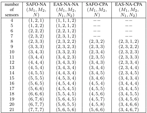
TABLE I
PARAMETER SETTING OF THE CORRESPONDING SPARSE ARRAYS.
number SAFO-NA EAS-NA-NA SAFO-CPA EAS-NA-CPA of (M1, M2, (M1, M2, (M1, M2, (M1, M2,
sensors N) N1, N2) N) N1, N2)
4 (1,2,1) (1,1,1,2) −− −−
5 (1,2,2) (1,2,1,2) −− −−
6 (2,2,2) (2,2,1,2) −− −−
7 (2,3,2) (2,3,1,2) −− −−
8 (2,3,3) (2,3,2,2) (2,3,2) (2,3,1,2)
9 (3,3,3) (2,3,2,3) (2,3,3) (2,3,2,2)
10 (3,4,3) (3,3,2,3) (2,3,4) (2,3,2,3)
11 (3,4,4) (3,4,2,3) (2,3,5) (2,3,3,3)
12 (4,4,4) (3,4,3,3) (3,4,3) (2,3,3,4)
13 (4,5,4) (3,4,3,4) (3,4,4) (2,3,4,4)
14 (4,5,5) (4,4,3,4) (3,4,5) (2,3,4,5)
15 (5,5,5) (4,5,3,4) (3,4,6) (3,4,3,4)
16 (5,6,5) (4,5,4,4) (4,5,4) (3,4,4,4)
17 (5,6,6) (4,5,4,5) (4,5,5) (3,4,4,5)
18 (6,6,6) (5,5,4,5) (4,5,6) (3,4,5,5)
19 (6,7,6) (5,6,4,5) (4,5,7) (3,4,5,6)
20 (6,7,7) (5,6,5,5) (4,5,8) (3,4,6,6)
21 (7,7,7) (5,6,5,6) (5,6,6) (3,4,6,7)
the four cases with different number of physical sensors and the corresponding parameter settings are provided in Tab. IV. We can see from the figure that, for the total number of physical sensorsL >4, the number of DOFs of EAS-NA-NA is always larger than the SAFO-NA structure, while EAS-NA-CPA outperforms the SAFO-CPA for L > 8. On the other hand, EAS-NA-CPA and SAFO-NA have a similar result and the CL number for the EAS-NA-CPA will exceeds that
of SAFO-NA for L > 16. The performance of EAS-NA-NA is the best of all, which greatly exceeds the other three structures forL >10. For example, forL= 18, the number of consecutive fourth-order lags are 2949, 1751, 1653and1101
for EAS-NA-NA, EAS-NA-CPA, SAFO-NA, and SAFO-CPA, respectively.
V. SIMULATIONRESULTS
CS-θ(degree)
-60 -40 -20 0 20 40 60
Normalized spectrum
[image:5.612.53.294.51.215.2]0 0.2 0.4 0.6 0.8 1
Fig. 2. DOA estimation result for the EAS-NA-NA array.
based DOA estimation algorithm is employed as in [22], [23], where the constrainedL1 norm minimization problem can be
solved using cvx, a package for specifying and solving convex problems [24], [25]. In the formulation, the full angle range from−90◦ to90◦is discretized with a step size of0.05◦. The sources are generated by fixing the magnitude and frequency of a complex baseband signal and then changing its phase randomly following a uniform distribution on[0,2π].
In the first simulation, we consider an EAS-NA-NA array with L = 6 sensors and the parameters are set to beM1 =
1 and M2 = N1 = N2 = 2, with P = {1,2,4} ·d and
ˆ
Q = {11,18,39} ·d. K = 41 narrowband source signals are uniformly distributed between −60◦ and 60◦. The input SNR is 0dB, and the number of snapshots for calculating the fourth-order cumulant matrix is 20000. The DOA estimation result is shown in Fig. 2. Clearly, all the sources have been distinguished successfully.
Now we compare the performance of two nested array based structures, EAS-NA-NA and SAFO-NA, and the two co-prime array based structures, EAS-NA-CPA and SAFO-CPA, all with L= 12physical sensors. The parameters for the EAS-NA-NA array are M2 = 4, M1 = N1 = N2 = 3, for the SAFO-NA array are M1 = M2 = N = 4, for the EAS-NA-CPA
array are M1 = 2, M2 =N1 = 3 and N2 = 4, and finally
for the SAFO-CPA array are M1 = N = 3,M2 = 4. By
calculation, the physical aperture for EAS-NA-NA is 371·d,
270·dfor SAFO-NA,241·dfor EAS-NA-CPA, and181·dfor SAFO-CPA. The number of source signals isK= 35and the number of snapshots for calculating the fourth-order cumulant matrix is10000. The root-mean-squared error (RMSE) results obtained through 500 Monte Carlo trials are shown in Fig. 3 with a varied input SNR.
Evidently, the higher the input SNR, the higher its esti-mation accuracy. The performance of the nested array based structures are better than the co-prime array based ones, while the EAS-NA-NA has achieved the best performance for the whole input SNR range, which is due to not only a higher number of DOFs provided by the EAS-NA structure, but also a larger aperture.
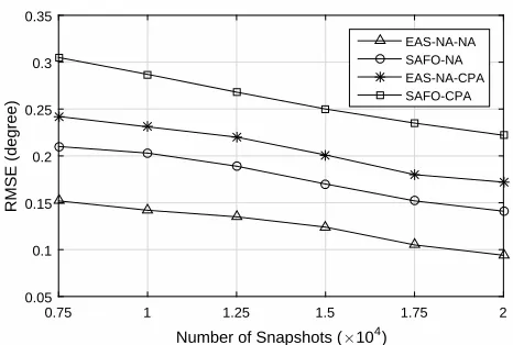
Next we fix the input SNR to 0dB, and change the number of snapshots. The RMSE results are shown in Fig.4, where we
SNR (dB)
-5 0 5 10 15 20
RMSE (degree)
0.14 0.16 0.18 0.2 0.22 0.24 0.26
0.28 EAS-NA-NA
[image:5.612.322.557.54.206.2]SAFO-NA EAS-NA-CPA SAFO-CPA
Fig. 3. RMSE results with respect to input SNR.
Number of Snapshots (×104)
0.75 1 1.25 1.5 1.75 2
RMSE (degree)
0.05 0.1 0.15 0.2 0.25 0.3 0.35
EAS-NA-NA SAFO-NA EAS-NA-CPA SAFO-CPA
Fig. 4. RMSE results with respect to snapshot number.
can see a similar trend and again the EAS-NA-NA structure has provided the best result for the considered full range of snapshot numbers.
VI. CONCLUSION
A general sparse array construction scheme called expand-ing and shift (EAS) has been proposed for maximizexpand-ing the continuous FODCA lags. It consists of two existing sparse sub-arrays, one withM physical sensors andCM consecutive
SODCA lags, while the other one withNphysical sensors and CN consecutive SODCA lags. Then, the second sub-array is
first expanded by increasing its unit spacing CM times and
then shifted to a position so that the two sub-arrays share one common physical sensor. As a result, with only M+N−1
physical sensors, CMCN consecutive FODCA lags can be
achieved. It is also shown that when the second sub-array is a two-level nested array, the number of consecutive FODCA lags can be further increased. As demonstrated by simulation results, the proposed EAS scheme has achieved a much better performance than two existing structures due to its higher number of DOFs and larger physical aperture.
REFERENCES
[image:5.612.322.555.251.408.2][2] R. T. Hoctor and S. A. Kassam, “The unifying role of the coarray in apeture synthesis for coherent and incoherent imaging,”Proceedings of the IEEE, vol. 78, no. 4, pp. 735 –752, Apr. 1990.
[3] P. Pal and P. P. Vaidyanathan, “Co-prime sampling and the music algorithm,” in IEEE Digital Signal Processing Workshop and IEEE Signal Processing Education Workshop(DSP/SPE), Sedona, AZ, January 2011, pp. 289–294.
[4] P. P. Vaidyanathan and P. Pal, “Sparse sensing with co-prime samplers and arrays,”IEEE Transactions on Signal Processing, vol. 59, no. 2, pp. 573–586, Feb. 2011.
[5] Y. M. Zhang, M. G. Amin, and B. Himed, “Sparsity-based DOA esti-mation using co-prime arrays,” inProc. IEEE International Conference on Acoustics, Speech, and Signal Processing, Vancouver, Canada, May 2013, pp. 3967–3971.
[6] P. Pal and P. P. Vaidyanathan, “Nested arrays: a novel approch to array processing with enhanced degrees of freedom,”IEEE Transactions on Signal Processing, vol. 58, no. 8, pp. 4167–4181, Aug. 2010. [7] Z. B. Shen, C. X. Dong, Y. Y. Dong, G. Q. Zhao, and L. Huang,
“Broadband DOA estimation based on nested arrays,” International Journal of Antennas and Propagation, vol. 2015, 2015.
[8] P. Pal and P. P. Vaidyanathan, “Coprime sampling and the MUSIC algorithm,” inProc. IEEE Digital Signal Processing Workshop and IEEE Signal Processing Education Workshop (DSP/SPE), Sedona, AZ, Jan. 2011, pp. 289–294.
[9] C.-L. Liu and P. P. Vaidyanathan, “Remarks on the spatial smoothing step in coarray MUSIC,” vol. 22, no. 9, pp. 1438–1442, Sep. 2015. [10] Q. Shen, W. Liu, W. Cui, S. L. Wu, Y. D. Zhang, and M. Amin,
“Low-complexity direction-of-arrival estimation based on wideband co-prime arrays,”IEEE Trans. Audio, Speech and Language Processing, vol. 23, pp. 1445–1456, September 2015.
[11] S. Qin, Y. D. Zhang, and M. G. Amin, “Generalized coprime array configurations for direction-of-arrival estimation,”IEEE Transactions on Signal Processing, vol. 63, no. 6, pp. 1377–1390, March 2015. [12] J. J. Cai, D. Bao, and P. Li, “Doa estimation via sparse recovering from
the smoothed covariance vector,”Journal of Systems Engineering and Electronics, vol. 27, no. 3, pp. 555–561, June 2016.
[13] Q. Shen, W. Liu, W. Cui, and S. L. Wu, “Underdetermined DOA estimation under the compressive sensing framework: A review,”IEEE Access, vol. 4, pp. 8865–8878, 2016.
[14] J. F. Cardoso and E. Moulines, “Asymptotic performance analysis of direction-finding algorithms based on fourth-order cumulants,” IEEE Transactions on Signal Processing, vol. 43, no. 1, pp. 214 –224, Jan. 1995.
[15] M. C. Dogan and J. M. Mendel, “Applications of cumulants to array pro-cessing.i.aperture extension and array calibration,”IEEE Transactions on Signal Processing, vol. 43, no. 5, pp. 1200 –1216, May 1995. [16] P. Chevalier and A. Ferreol, “On the virtual array concept for the
fourth-order direction finding promblem,”IEEE Transactions on Signal Processing, vol. 47, no. 9, pp. 2592 –2595, Sep. 1999.
[17] P. Chevalier, L. Albera, A. F´err´eol, and P. Comon, “On the virtual array concept for higher order array processing,” vol. 53, no. 4, pp. 1254– 1271, Apr. 2005.
[18] P. Cardoso and A. Ferreol, “High-resolution direction finding from higher order statistics: The 2q-music algorithm,”IEEE Transactions on Signal Processing, vol. 54, no. 8, pp. 2986 –2997, Aug. 2006. [19] G. Birot, L. Albera, and P. Chevalier, “Sequential high-resolution
direc-tion finding from higher order statistics,”IEEE Transactions on Signal Processing, vol. 58, no. 8, pp. 4144–4155, Aug 2010.
[20] P. Pal and P. P. Vaidyanathan, “Multiple level nested array: an efficient geometry for 2qth order cumulant based array processing,”IEEE Trans-actions on Signal Processing, vol. 60, no. 3, pp. 1253–1269, Mar. 2012. [21] W. K. Ma, T. H. Hsieh, and C. Y. Chi, “DOA estimation of quasi-stationary signals with less sensors than sources and unknown spatial noise covariance: a khatri–rao subspace approach,”IEEE Transactions on Signal Processing, vol. 58, no. 4, pp. 2168–2180, April 2010. [22] Q. Shen, W. Liu, W. Cui, and S. L. Wu, “Extension of co-prime arrays
based on the fourth-order difference co-array concept,” IEEE Signal Processing Letters, vol. 23, no. 5, pp. 615–619, May 2016.
[23] ——, “Extension of nested arrays with the fourth-order difference co-array enhancement,” in The 41st IEEE International Conference on Acoustics, Speech and Signal Processing, Shanghai, China, March 2016, pp. 2991–2995.
[24] C. Research, “CVX: Matlab software for disciplined convex program-ming, version 2.0 beta,” http://cvxr.com/cvx, September 2012. [25] M. Grant and S. Boyd, “Graph implementations for nonsmooth convex
programs,” inRecent Advances in Learning and Control, ser. Lecture Notes in Control and Information Sciences, V. Blondel, S. Boyd, and