Estimation of Mean Transition Time using Markov Model and Comparison of risk factors of malnutrition using Markov Regression to Generalized Estimating Equations and Random Effects Model in a Longitudinal Study.

(1)

Estimation of Mean Transition Time using Markov Model and Comparison of risk factors of malnutrition using Markov Regression to Generalized Estimating Equations

and Random Effects Model in a Longitudinal Study

Thesis submitted to

The Tamil Nadu Dr. M.G.R. Medical University

For the degree of Doctor of Philosophy

by Visalakshi J

Department of Biostatistics Christian Medical College

(2)

6. RESULTS ... 82

6.1 Prevalence, Incidence and Cumulative Incidence of Malnutrition ... 82

6.1.1 Prevalence, Incidence and Cumulative Incidence of Malnutrition using BMI classification ... 82

6.1.2 Prevalence, Incidence and Cumulative Incidence of Acute Malnutrition using Weight-for-age (underweight) classification ... 83

6.1.3 Prevalence, Incidence and Cumulative Incidence of Chronic Malnutrition (stunting) using Height-for-age classification ... 83

6.1.4. Prevalence, Incidence and Cumulative Incidence of Malnutrition (wasted) using Weight-for-height classification ... 84

6.2 Risk Factor Analysis ... 85

6.2.1. Repeated Measure Analysis using Generalized Estimating Equations (GEE) using BMI classification ... 85

6.3 Markov Chain ... 86

(4)

6.3.2 Transition Probability and Mean Passage time for malnutrition by sex according to

BMI classification ... 87

6.3.3 Transition Probability and Mean Passage Time for malnutrition by area of residence according to BMI classification ... 88

6.3.4 Transition Probability and Mean Passage Time for malnutrition by presence of a separate kitchen according to BMI classification ... 89

6.3.5 Transition Probability and Mean Passage Time for malnutrition by defecation according to BMI classification ... 91

6.3.6 Transition Probability and Mean Passage Time for malnutrition by type of fuel used for cooking according to BMI classification ... 93

6.4 Markov Regression ... 95

6.4.1 Markov Regression using Transition Probabilities for malnutrition using BMI classification ... 95

6.4.2 Transition Intensity Matrix for malnutrition using BMI classification ... 98

6.5 Generalized Estimating Equations for Height-for-Age classification ... 100

6.6 Markov Chain using Height-for-Age classification ... 102

6.7. Markov Regression Analysis using transition probabilities for Height-for-Age classification ... 109

6.8. Markov Regression Analysis using intensity rate for Height-for-Age classification ... 112

6.9 Comparison of GEE, Markov Regression with transition probabilities and transition intensity rates for malnutrition using BMI classification ... 115

6.10. Comparison of GEE, Markov Regression with transition probabilities and transition intensity rates for malnutrition using Height-for-Age classification ... 117

6.11 Comparison of coverage probability and length of the confidence interval ... 119

7. DISCUSSION ... 120

8. SUMMARY AND CONCLUSION ... 130

9. IMPACT OF THE STUDY ... 135

10. REFERENCES ... 137

(5)

(6)

~ 1 ~

1. INTRODUCTION

1.1 Malnutrition

:

(7)

~ 2 ~

1.2 Risk Factors associated with Malnutrition

:

(8)

~ 3 ~

mainly due to high low birthweight rates, poor infant and young child feeding and caring practices. Malnutrition is an important indicator of child health. A significant contributing factor to infant and child mortality, poor nutritional status during childhood also has implications for adult economic achievement and health (8). A study from South India suggested that the risk factors for severe malnutrition were found to be low mother’s education, low family income, more among boys, use of firewood or coal for cooking and defecation within premises (9).

1.3 Generalized Estimating Equations

:

Generalized Estimating equations (GEE) are extensions of linear regression analysis which are applied when there are repeated observations (responses) obtained from the same individual. As the response from each individual is obtained over time, these observations are not independent and hence the usual regression analysis is not applicable. There is considerable correlation as the responses are obtained from the same individual. Hence the GEE method accounts the correlation as a nuisance parameter and thereby included in the model as a covariate. The correlation structure is decided a prior which may be a difficult task especially when the outcome is a categorical variable. However, GEE is still robust for a wrong choice of correlation.

1.4 Random Effects Model or Multilevel Modeling (MLM)

:

(9)

~ 4 ~

individual. In such a situation, individuals are cluster and each unit of repeated measurement within that individual are the next level.

1.5 Markov Chain

:

Mathematical models represent real world problems or phenomena by formal system (10). They offer several advantages over empirical studies, as well as a number of disadvantages. Among the advantages are the identification of the variables in a quantitative problem that have the most impact on the system, and in particular the ability to ask “What if?” questions of the model. The Markov chain model has several attractive features that stem from the central assumption of the model: the probability of arriving in stat j, given that the process is in state i at time T, (known as a transition probability), is determined only by i and j. This strong assumption yield a homogeneous Markov Chain. Chronic diseases such as neurologic, cardiovascular and rheumatic disorders seem to obey the Markov assumption. The Markov model uses data on the probability of transition from one clinical status or disease state to another disease state to derive under certain assumptions, the duration of time spent in each disease state. It is possible to determine the future probability that a patient will be in each disease state from information on the current disease state.

Silverstein et al. demonstrated that the natural history of systemic lupus erythematosus in fact can be modeled as a homogeneous chain, and thus validate an assumption made by earlier users of the Markov model.

(10)

~ 5 ~

Another feature of Markov models is the natural division of a population into cohorts of different health states. With this allocation, and measure of QOL superimposed on the model, one can calculate state specific measures of health status or utility. These results can be incorporated into clinical decision analyses, using the Markov chain as a utility structure. Such modeling is particularly appropriate for cost-effectiveness analysis, wherein resources and health benefits are accrued incrementally, rather than summarized at the end of the model. The ideal population upon which to perform stochastic modeling is a true inception cohort, but such investigations are now just underway.

1.5.1 Mean first passage and Sojourn time: Mean First Passage Time:

(11)

~ 6 ~ Sojourn time:

Using the transition probabilities, it is imperative to estimate the expected duration stay in each state of disease. For example, how long a child is expected to be in severe malnutrition or in normal state. This can be done for both Markov models with absorbing and non-absorbing state. This will help the therapists to plan treatment options for specific duration to reverse the disease progression.

1.6 Markov Regression

:

In usual regression the hypothesized variables are associated with the outcome after adjusting for other known risk factors and confounders. In Markov regression the concept of current disease state depends on the previous state of the disease. That is, when we model the duration of disease and the probability of transition from one state to another, the conditional probability concept or the hazard concept is incorporated in the regression analysis. Thus in chronic disease epidemiology, if the current state of the disease depends on the previous state, then it is appropriate to consider Markov regression. This also adjusts for other risk factors, confounders, besides the previous state information.

(12)

~ 7 ~

transition between various states, estimating the probability of transition from one state to another within a specific time period, or estimating the average period of single stay in a state (mean sojourn time) and also risk factors.

(13)

(14)

~ 8 ~

2. AIMS AND OBJECTIVES

The main aim of the thesis is to find if malnutrition was associated with any of household factors from which the child was taken for the study such as type of fuel used for cooking, education of the mother and father, sex of the child, etc.

The objectives of the thesis are:

1. To estimate the first mean passage time which indicates the average time spent by a child to move from one state to another

2. To find risk factors of using GEE and Random effects model

3. To find risk factors of protein energy malnutrition using Markov regression with transition probabilities

4. To find the risk factors using Markov Regression with transition intensity rates

(15)

(16)

~ 9 ~

3. REVIEW OF LITERATURE

3.1 Definition of Malnutrition:

World Health Organization (WHO) defined the term ‘malnutrition’ as a condition that refers to a number of diseases each with a specific cause related to the cellular imbalance of one or more nutrients like protein, iodine and/or calcium and the body’s demand to ensure growth, maintenance and proper functioning. Malnutrition can disable, maim or even kill. In the past few years, there is an economic growth and seems to be an improvement in food supplies, health conditions, availability of educational resources and social services but malnutrition seems to persisting virtually in all countries of the world (1).

3.1.1 Indices for measuring Malnutrition:

(17)

~ 10 ~

mass in relation to the body length and describes the current nutritional status. Children below -3SD are considered severely thin (wasted) and are acutely malnourished. Weight-for-age is a composite index of height-for-age and weight-for-height. It takes into account both acute and chronic malnutrition. Children below -3SD are considered to be severely underweight. An article from Chile had suggested BMI Z scores as an index of underweight. The classification using BMI Z scores have been used recently in clinical settings. Children whose BMI Z score was less than -3SD were considered as severely underweight (15).

3.2 Prevalence of Malnutrition:

In 1990, the WHO fact sheet reported that only 53 developing countries had reliable national data on the prevalence of underweight in young children; by 1995, 97 countries had such data, and 95 countries also had data on stunting and wasting. It is estimated that more than half of the young children in south Asia suffer from protein energy malnutrition, which is about five times the prevalence in the Western hemisphere, at least three times the prevalence in the Middle East and more than twice that of east Asia. Estimated for sub-Saharan Africa indicate that the prevalence is approximately 30%. In some regions, such as sub-Saharan Africa and south Asia, stagnation of nutritional improvement combined with a rapid rise in population has resulted in an actual increase in the total number of malnourished children. Currently, over one thirds of the world’s malnourished children live in Asia (especially south Asia), followed by Africa and Latin America (1).

(18)

~ 11 ~

and a quarter of all births are low weight. These high levels of malnutrition contribute to about half of the 740,000 children deaths that occur every year in Pakistan (16).

Protein-Energy malnutrition (PEM) is one of the most serious health problems in Bangladesh too where PEM accounts for 35% of deaths of children aged less than five years and total burden of disease. There were earlier reports that were reported in the same article that, severely underweight children aged 6-59 months had more than eight fold increased mortality (4). Another study reported that India has the highest percentages of undernourished children in the world (17).

Malnutrition is also a significant problem in older children. It was indicated that there is very little known about the state of nutrition but some studies conducted in 1980s indicate that malnutrition is a significant problem with prevalence ranging from 47-70% in male school children in rural Pakistan. Within 7-10 year age, 36% were underweight, 39% stunted and 20% wasted. The prevalence of underweight in children between 5-7 years was 26% underweight, 32% stunted and 8% wasted (18).

The national nutrition survey in Bangladesh found that 29% of under-five children were moderately underweight and 12% were severely underweight according to weight-for-age Zscores. The prevalence of underweight decreased over the follow-up from the years 1987 to 2002 in a national school-based annual population surveys in 6 year old children (15).

(19)

~ 12 ~ 3.3 Risk Factors:

Most of the studies reviewed addressed many risk factors for the prevalence of malnutrition among children. A lot of studies reported that malnutrition was mainly a severe problem in resource poor developing countries.

(20)

~ 13 ~

(21)

~ 14 ~

(22)

~ 15 ~

The significant risk factors that were associated with weight-for-age were birth weight, number of pregnancies, birth order, body mass index of the mother and maternal weight. The significant factors associated with weight-for-height were birth weight, age of mother at birth of the child, The birth weight had shown a relative risk (RR) of 5.7 with 95% confidence interval to be 2.1-15.2. The factors associated with height-for-age were also birth weight, age of the mother at birth, maternal height, Body mass index of the mother, birthplace of mother and father. This study had birth weight as a factor that was important for weight-for-age, weight-for-height and height-for-age indices (22).

(23)

~ 16 ~

above factors were unadjusted factors. The adjusted factors that contributed for underweight were teen aged mother, education of the mother, predominant breastfeeding for 4 months, education of the father, monthly family income, undernourished mother, shorter mother and father’s job category. If the mother was a teen aged person then there was 3 times the odds of having underweight child. If the mother was undernourished, then there was nearly 4 times the odds of having underweight baby. If the mother was illiterate or had less than five years of education, then there was nearly 3 times the odds of having underweight baby (4).

(24)

~ 17 ~

the defecation was within the premises then there was more likely that the child had moderate or severe malnutrition as compared to defecation done in open fields. The other interesting finding was type of roof. If the type of roof was thatched, then there was a high odds of having moderate or severe malnourished child as compared to houses that had RCC or pukka type roofs (9).

3.4 Generalized Estimating Equations:

Need to perform Generalized Estimating Equations (GEE):

The generalized estimating equations (GEE) method, an extension of the quasi-likelihood approach, is being increasingly used to analyze longitudinal and other correlated data, especially when they are binary or in the form of counts consist of the age- and sex-standardized heights and data on the covariates gender and socioeconomic status) of 144 children in a sample of 54 randomly selected households in Mexico. The results presented as Odds ratio (OR) were compared using the logistic regression analysis. The result using the logistic regression analysis was found to be 9 whereas after adjusting for the correlation using GEE it was found to be 5.4 (23).

(25)

~ 18 ~

A study explains the structure of GEE with count responses. The main challenge mainly in a longitudinal data is when data are correlated within subject such as that provided in longitudinal studies and also in which data are clustered within subgroups. Failure to incorporate correlation of responses can lead to incorrect estimation of regression model parameters especially when the correlations are very large. This incorrect estimation has been demonstrated using a study that collected data from a laboratory that involved assembling Lego objects over five consecutive sessions. The responses are not normally distributed because they consist of count of the number of trips out of the room. The other variables that were correlated to the outcome were the object that needs to be assembled, the size of the object. The data was analyzed using Poisson distribution with independent correlation structure, Poisson distribution with unstructured correlation and Poisson distribution with one dependent autoregressive correlation. (25).

Working Correlation structures and its bounds:

In a longitudinal data analysis using GEE, the variance is considered as nuisance parameter. In some situations, it is important to understand the structure of the variability the same as understanding the mean structure. Moreover, treating the variance structure as a nuisance parameter can lead to misleading conclusions (26).

(26)

~ 19 ~

(27)

~ 20 ~

repeated measurements ranged from AR(1) to compound symmetry in graded steps, whereas the GEE and GLMM formulations restricted the respective error structure models to be either AR(1), compound symmetry (CS), or unstructured (UN). The GEE-based tests utilizing empirical sandwich estimator criteria were documented to be relatively insensitive to misspecification of the covariance structure models, whereas GLMM tests which relied on restricted maximum likelihood (REML) were highly sensitive to relatively modest misspecification of the error correlation structure even though normality, variance homogeneity, and linearity were not an issue in the simulated data. Goodness-of-fit statistics were of little utility in identifying cases in which relatively minor misspecification of the GLMM error structure model resulted in inadequate alpha protection for tests of the equal slopes hypothesis. Both GEE and GLMM formulations that relied on unstructured (UN) error model specification produced non-conservative results regardless of the actual correlation structure of the repeated measurements. A random coefficients model produced robust tests with competitive power across all conditions examined (28).

Some authors have argued that Chaganty and Joe (2004, 2006) have argued that the GEE correlation structures are not correlations at all, but rather weighted matrices. Their claim is based on the supposition that the range of correlations for multivariable binary distributions – i.e., Bernoulli distributions – are based on the marginal means, which they believe preclude the working correlation from being the true correlation of the data (29, 30).

(28)

~ 21 ~

responses when an individual is measured repeatedly over time. The data used for the comparison was from the Amsterdam Growth and Health study investigating the longitudinal relationship between lifestyle and health in adolescence and young adulthood. There were six measurements on 147 observations. The main hypothesis was to find the relationship between serum cholesterol levels and physical fitness at baseline, body fatness and smoking behavior classified as smoking or non-smoking and gender. The serum cholesterol levels were expressed in mmol/liter or categorized into upper and lower tertiles respectively. The results were compared using the continuous outcome and binary outcome between GEE and random coefficient model. The results from the study was that the GEE and random coefficient model for continuous outcome was similar but there was a difference in the standard errors when dichotomous outcome was considered for analysis (31).

Choice of Correlation Structure:

(29)

~ 22 ~

There was a study that compared several approaches to select the best working correlation structure and it was suggested that all approaches be used to select correlation structure and then decide on the best correlation and the problem spreads more when there is a small sample size (33).

Quasi Likelihood estimation:

Correlated response data are common in biomedical studies. Regression analysis based on the GEE is an increasingly important method for such data. However, there seem to be few model-selection criteria available in GEE. The well-known Akaike Information Criterion (AIC) cannot be directly applied since AIC is based on maximum likelihood estimation while GEE is non-likelihood based. The authors proposed a modification to AIC, where the non-likelihood is replaced by the quasi likelihood and a proper adjustment is made for the penalty term. Its performance is investigated through simulation studies. For illustration, the method is applied to a real data set (34).

(30)

~ 23 ~

The generalized estimating equation is a popular method for analyzing correlated response data. It is important to determine a proper working correlation matrix at the time of applying the generalized estimating equation since an improper selection sometimes results in inefficient parameter estimates. The authors proposed a criterion for the selection of an appropriate working correlation structure. The proposed criterion is based on a statistic to test the hypothesis that the covariance matrix equals a given matrix, and also measures the discrepancy between the covariance matrix estimator and the specified working covariance matrix. They evaluated the performance of the proposed criterion through simulation studies assuming that for each subject, the number of observations remains the same. The results revealed that when the proposed criterion was adopted, the proportion of selecting a true correlation structure was generally higher than that when other competing approaches were adopted (36).

(31)

~ 24 ~

obtained when a ‘Gaussian estimation’ pseudo likelihood procedure is used with an AR(1) structure (37).

The GEE technique is often used in longitudinal data modeling, where investigators are interested in population-averaged effects of covariates on responses of interest. GEE involves specifying a model relating covariates to outcomes and a plausible correlation structure between responses at different time periods. While GEE parameter estimates are consistent irrespective of the true underlying correlation structure, the method has some limitations that include challenges with model selection due to lack of absolute goodness-of-fit tests to aid comparisons among several plausible models. The quadratic inference functions (QIF) method extends the capabilities of GEE, while also addressing some GEE limitations (38).

There was a study that showed the difficulties with GEE particularly with logistic regression GEE analysis. There are also other authors who have considered these claims to be based more on semantics than on statistics especially for binary response models (39).

3.5 Random Effects Model:

When is a Random effects model applied:

(32)

~ 25 ~

large cohort study. The authors also applied Bayesian estimation methods to fit discrete-mixture alternative to the standard logistic-normal model and posterior predictive checking was used to assess the model fit. The authors described surprising parallels in the parameter estimates from the logistic-normal and mixture models and used them to question the interpretability of the subject specific regression coefficients from the standard multilevel approach. Positive predictive checks suggested a serious lack of fit of both multilevel models. The authors expressed that lessons learnt from the case study provided guidance for further investigations (40).

(33)

~ 26 ~

models provide the variance from which correlation termed as Intraclass correlation coefficient (ICC) is calculated. Maximum likelihood is the standard methods of estimation for linear mixed models. However, evaluation of likelihood is computationally difficult. The log likelihood is maximized using numerical integration (41).

Intraclass Correlation Coefficient (ICC):

(34)

~ 27 ~

clinics are more similar to each other than to those at other clinics. Had the researchers ignored the hierarchical structure of the data and used traditional analytic approaches, they would have erroneously concluded that physician advice had little or no influence on patient alcohol consumption behavior. On the other hand, all the HLMs that assess the relationship between physician time advising patients on alcohol consumption and patient behavior lead to the conclusion that physician advice is effective, at least in some settings (42).

An adolescent study was done that included 8th and 10th grades with varying amounts of cigarette smoking experience. These were categorized into three categories such as < 6cigarettes, 6-99 and 100+ cigarettes. The outcome was physiological sensation change categorized into five ordered categories such as -2, -1, 0, 1 and 2. The ICC was found to be 0.44 suggesting that there was correlation within subjects. The study showed that physiological sensation diminishes as smoking level increases (43).

Estimation procedures for count data in random effect models:

In the social and health sciences, data are often structured hierarchically, with individuals nested within groups. This was presented using dyadic data. Dyadic data represent a special case of hierarchically clustered data, with individuals nested within dyads. Dyads constitute a special case of hierarchically structured data with variation at both the individual and dyadic level. Analyses of data from dyads pose several challenges due to the interdependence between members within dyads and issues related to small group sizes. Multilevel analytic techniques have been developed and applied to dyadic data in an attempt to resolve these issues. In this article, the authors described a set of analyses for modeling individual- and dyad-level influences

(35)

~ 28 ~

limitations of such an approach. For illustrative purposes, the authors applied these techniques to estimate individual-dyad-level predictors of viral hepatitis C infection among heterosexual couples in East Harlem, New York City (44).

Least squares analyses (e.g., ANOVAs, linear regressions) of hierarchical data leads to Type-I error rates that depart severely from the nominal Type-I error rate assumed. Thus, when least squares methods are used to analyze hierarchical data coming from designs in which some groups are assigned to the treatment condition, and others to the control condition (i.e., the widely used groups nested under treatment experimental design), the Type-I error rate is seriously inflated, leading too often to the incorrect rejection of the null hypothesis (i.e., the incorrect conclusion of an effect of the treatment). To highlight the severity of the problem, a paper presented simulations showing how the Type-I error rate is affected under different conditions of intraclass correlation and sample size. For all simulations the Type-I error rate after application of the popular correction is also considered, and the limitations of this correction technique discussed. They concluded with suggestions on how one should collect and analyze data bearing a hierarchical structure (45).

(36)

~ 29 ~

effect, the decision about the statistical significance of the test statistic changes. When there is a failure to account for the clustered nature of the data, it was concluded that the difference between the two groups is statistically significant. However, once they adjusted the standard error for the design effect, the difference is no longer statistically significant (47).

Comparison of Fixed Effects, GEE and Random Effects model:

A study reported the differences between fixed effects, random effects and GEE analysis. This article reported the underlying assumptions to assess the covariate effects on the mean of continuous, dichotomous or count outcomes. This paper reports the structural differences and similarities of the random effects, the linear mixed model, the fixed effects and generalized estimating equations in a longitudinal data. Let the random draw from a population of interest be (Yi_,

X

i

),

where I denotes the sampling unit = , , … the time-ordered × 1 vector

of responses and = , , … an × matrix of explanatory variables with Xij a

× 1 vector associated with the response Yij. The conditional mean vector and covariance

matrix are respectively, = (|) and = (− )( − )|. In the above notation, each component of the conditional mean = (|) is a function of all the covariates. The total number of observations in the sample is = ∑ _! . Let g be a known link function such that " = # where # = (#, … #_$) is a pX1 vector of unknown parameters. Whereas the mean depends on β, the covariance matrix Vi may depend on β and perhaps additional

(37)

~ 30 ~

Marginal Model: This specifies only the conditional mean = (|) but treats the parameters in Vi as nuisance parameters. A distribution function in the exponential family

usually suggests the form of mean and variance of Yij.

Random Effects model: In this model, correlation is induced through an unobserved heterogeneity ζi in the conditional mean specification n = (|, %). The random coefficient model will also fall under this umbrella allowing one to acknowledge dependencies at different levels of a hierarchy (48).

(38)

~ 31 ~

models. The results do not provide final answers to the two questions posed, but we expect that lessons learned from the case study will provide general guidance for further investigation of these important issues (40).

Several approaches have been proposed to model binary outcomes that arise from longitudinal studies. Most of the approaches can be grouped into two classes: the population-averaged and subject-specific approaches. The generalized estimating equations (GEE) method is commonly used to estimate population-averaged effects, while random-effects logistic models can be used to estimate subject-specific effects. However, it is not clear to many epidemiologists how these two methods relate to one another or how these methods relate to more traditional stratified analysis and standard logistic models. The authors address these issues in the context of a longitudinal smoking prevention trial, the Midwestern Prevention Project. In particular, the authors compare results from stratified analysis, standard logistic models, conditional logistic models, the GEE models, and random-effects models by analyzing a binary outcome from two and seven repeated measurements, respectively. In the comparison, the authors focus on the interpretation of both time-varying and time-invariant covariates under different models. Implications of these methods for epidemiologic research have been discussed which found that both estimates for random effects and standard errors were larger than GEE model although the test statistic results were similar (49).

(39)

~ 32 ~

regression (CLR) and generalized estimation equations (GEE) on the measures of power, type I error, estimation bias and standard error. The results indicated that rMLM was a valid test of association in the presence of linkage using sibship data. The advantages of rMLM became more evident when the data contained concordant sibships. Compared to GEE, rMLM had less underestimated odds ratio (50).

Diagnostic issues in Random effect models:

Commonly applied diagnostic procedures in random-coefficient (multilevel) analysis are based on an inspection of the residuals, motivated by established procedures for ordinary regression. The deficiencies of such procedures are discussed and an alternative based on simulation from the fitted model (parametric bootstrap) is proposed. Although computationally intensive, the method proposed requires little programming effort additional to implementing the model fitting procedure. It can be tailored for specific kinds of outliers. Some computationally less demanding alternatives are described (51).

3.6 Markov Chain:

(40)

~ 33 ~

asymptomatic to symptomatic NIDDM was 2.27% implying that there was a high risk of dying from NIDDM for subjects with symptomatic NIDDM (52). This paper, however, is based on absorbing state where there is no possible transition from death state. Therefore there is a need for non-absorbing state model.

For many recurrent events, a change in state during a sufficiently narrow time span usually involves a move to next state only. For example, the person with no headache during one interval is more likely during the next span of time to have a slight headache than a severe headache. A Markov chain is a stochastic model that describes the probabilities of transition among sites of a system. The assumption that characterizes a Markov chain is that the transitional probability is completely determined by the present state of the system. A headache diary was completed by 177 female and 57 male headache patients. The patients were asked to record their level of headache during each 24-hr interval for 28 days. The main aim of the study was to see if the movement from time t to t+1 was different for males and females. This was tested using log linear model. The G2 = 25.17 for 9 degrees of freedom suggesting that there was a difference in the transition probability for males and females (53). This study has not estimated the likely duration of stay in each state of headache transition which may be of clinical importance.

(41)

~ 34 ~

A study was conducted to describe the lifetime clinical course and costs of Crohn’s disease in a 24-year population-based inception cohort of patients with Crohn’s disease in Olmsted county. The disease states were defined by medical and surgical treatment. A Markov model analysis calculated time in each disease state and presented value of excess lifetime costs in comparison with an age- and sex matched cohort (54).

A Markov model of prognosis was evaluated by comparing the duration of disease activity states and life expectancy with Kaplan Meier curves for 98 patients with systemic lupus erythematous with 1080 patient years of observations. A four state homogenous Markov chain was constructed to determine the transition probabilities between the disease states. The proportion of the patient population in each disease state over time provided a convenient graphic summary of the natural history of SLE from which the Kaplan Meier survival curves were obtained. A Markov model yielded a clinically useful description of outcome for multistate disease (55).

(42)

~ 35 ~

The oval represents the patient being in one of the three ovals (upper row) and transitions that occur over a fixed time interval i are illustrated by the arrows from i to i+1. It is possible to leave WELL or ILL via a transition and hence are termed as Non-absorbing states where as once DEAD state is reached no possible transitions can be made and hence is an absorbing state. This paper has described the constant transition probabilities that are possible only with Markov chain model. The matrix formulation has four important sections.

The section labeled Q which reflects the probability of not being absorbed and the probability of being in the WELL state is sum of the four probabilities of the elements. Each element is

WELL

WELL ILL

DEAD

ILL Time i

Time i+1 Pwd

Pwi Pww

Pii

Pid

(43)

~ 36 ~

subtracted from a corresponding element in another 2X2 matrix of ones on the diagonal and zeros elsewhere. Matrix N is the fundamental matrix of absorbing Markov chain and has its elements by column the expected time in each of absorption state given the starting state corresponding to the row of N matrix which is displayed in the figure below which represents the single step transition between and within absorbing and transient states (10).

Another study reported the mean sojourn time which is the time spent in the preclinical detectable phase for chronic disease like breast cancer that plays an important role in the design and assessment of screening programs. This paper developed two-parameter Markov chain model and the model was developed explicitly to estimate the preclinical incidence rate and the rate of transition from preclinical to clinical state without using control data. Using this method to the data from Swedish two county study of breast cancer screening in the age group 70-74, the mean sojourn time was found to be 2.3 with 95 percent confidence interval ranging from 2.1 – 2.5 which was close to the result based on the traditional method however, the 95 percent confidence interval was narrower using Markov model. The reason for greater precision of the latter is the fuller use of all temporal data since the continuous exact times to events are used in our method instead of grouping them as in the traditional method (56). This paper presented the sojourn time but did not explain the transition time from one clinical state to another.

(44)

~ 37 ~

13.9 years and it was also found that proteinuria caused a 50% reduction in the life expectancy but increased disease activity at onset did not predispose to a poor outcome (57).

A study considered the estimation of the intensity and survival functions for a continuous time progressive three-state semi-Markov model with intermittently observed data. The estimator of the intensity function is defined nonparametrically as the maximum of a penalized likelihood. Thus the authors obtained smooth estimates of the intensity and survival functions. This approach also accommodated complex observation schemes such as truncation and interval censoring. The method is illustrated with a study of hemophiliacs infected by HIV. The intensity functions and the cumulative distribution functions for the time to infection and for the time to AIDS are estimated. Covariates can easily be incorporated into the model (58). This study explains for continuous time Markov model.

3.7 Markov Regression:

(45)

~ 38 ~

procedure changed substantially over the 7 years of data collection, a feature that is not captured using standard regression modeling (59). However, this approach may be intensive in computing and may have problem in generalizing.

A study describes the application of a multi-state model to diabetic retinopathy under the assumption that a continuous time Markov process determines the transition times between disease stages. There are three transient states that represented the early stages of retinopathy and one final absorbing state that represented the irreversible stage of retinopathy. Using a model with covariables, the authors explored the effects of factors that influenced the onset, progression and regression of diabetic retinopathy among subjects with insulin-dependent diabetes mellitus. The study also had time – dependent covariables in the model assuming that the covariables remained constant between two observations. The authors also demonstrated survival curves from each stage of the disease and for any combination of the risk factors (60). This was applied for absorbing state Markov model.

(46)

~ 39 ~

transition rates. The multivariable analysis showed that baseline functional status had an effect from state 2 to state 3 (HR: 0.14; 0.06 -0.25). Size of the infarct showed an effect on transition rate from state 1 to state 2 with hazard ratio (HR) 2.3 (1.6-3.0) (61).

A study on liver fibrosis evolution in HIV-HBV-coinfected patients treated with tenofovir disoproxil fumarate (TDF) was conducted. The effect of TDF on liver fibrosis in 148 HIV-HBV-coinfected patients was prospectively evaluated using Fibrometer scores and liver biopsies in a subset of patients. The mean change from baseline in Fibrometer score was modelled using a GEE and a homogeneous continuous-time Markov models were used to study risk factors for regression or progression of liver fibrosis. It was found that the median follow-up of patients treated with TDF was 29.5 months (25th-75th percentile 20.9-38.1). In patients with a baseline fibrosis score of F3-F4, Fibrometer score decreased with a triphasic shape (Fibrometer change at 12, 24 and 36 months after TDF initiation was -0.079, -0.069 and -0.102, respectively). Progression in fibrosis score over time was influenced by age, alcohol consumption, low CD4(+) T-cell count and HCV coinfection, whereas HDV coinfection and longer duration of HBV infection prevented fibrosis regression. No influence of antiretrovirals other than TDF was found (62). Continuous time Markov models, and the advantages over survival models need to be explored further in medical field.

(47)

~ 40 ~

found that a patient who was in the transitional state had 11% chance of being in the stable state at the end of 1 month, 5% chance of being in the end-of-life state at the end of 1 month, 24% chance of being dead at the end of this time There was 0.8% chance of death for a patient in the stable state at the end of 1 month where as 15% chance of death if the patient was in the stable state at the end of 6 months (63).

A longitudinal study that compared Markov model regression model, markov regression model with random effects and a mover-stayer model to find the risk factors for transition in Bacterial Vaginosis among women. The study showed that Markov regression model found a poor fit while Markov regression with random effects that accounted for additional unexplained heterogeneity had better fit to the data. The study found that transition models that accounted for additional heterogeneity provided an attractive approach for describing the effect of covariates on the natural history of BV (64).

There was a study that was conducted to find the potential effects of interventions on cervical cancer. The authors constructed a Markov state-transition model of a cohort of HIV positive women in Cameroon. They examined the potential impact, on cumulative cervical cancer mortality of four possible scenarios: when no HAART and no screening was present (NHNS), HAART and no screening (HNS), HAART and screening once on HAART initiation (HSHI) and HAART screening once at age 35 (HS35). The model projected that compared to NHNS, lifetime cumulative cervical cancer mortality approximately doubled with HNS (65).

(48)

~ 41 ~

main, quadratic and interaction effects. All effects in the model were cross-validated using the second subsample. Depression was found to be a strong predictor of suicidality; alcohol abuse was not a predictor. Both maternal and paternal love also predicted suicidality; the former had an indirect effect via depression and the latter a direct effect. Early experiences with violence showed both a direct and indirect association with suicidality. In addition to depression being a predictor for suicidality, various pathways connect suicidality with early childhood experiences (66).

(49)

(50)

~ 42 ~

4. SCOPE AND PLAN OF WORK

(51)

~ 43 ~

which deals with identifying and excluding the exact amount of correlation within individuals. Thus the usual GEE or MLM approach is expected to have wider standard errors (SE) as compared to Markov Regression (MR) models. Therefore there is a scope to find more number of risk factors as significant as compared to GEE or MLM models. However, the wider SE implying wider Confidence Intervals (CI) has to be shown as a consistent criteria and this can be shown through simulations. Hence, the coverage probabilities that the CIs could have, based on both methods, will provide us to suggest a best method. If expectation is that the MR shows to be a better method then this could change the practice.

(52)

~ 44 ~

(53)

(54)

~ 45 ~

5. MATERIALS AND METHODS

5.1. Data

:

During 1982, seven localities and 22 villages were selected for this study. These localities and villages were selected from Vellore town and KV Kuppam development block sampling frames respectively. All children aged 5-7 years were screened for signs of malnutrition by consultant pediatricians. The children from rural and urban areas of Vellore town were screened at baseline and followed up for every six months for 7 times. The anthropometric data were collected by two Anthropologists independently and care was taken to reduce intra and inter observer variability. Inter and intra observer variation was handled by standardizing the procedure.

5.2. Malnutrition classification

:

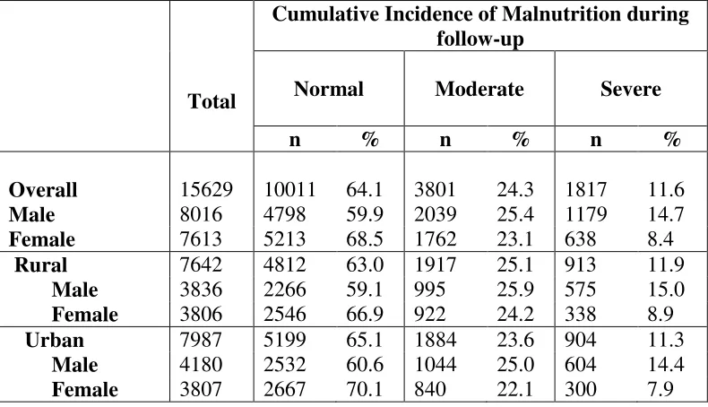
Malnutrition was assessed based on the indicators which are BMI Z scores, Height-for-age. The BMI Z scores were classified as “normal” if the BMI Z scores were >-2 standard deviations, “moderate” when Z scores were between -2 and -3 standard deviations and, “severe” if the Z scores were <-3 standard deviations (67). EPIINFO software was used to compute Z scores for every follow-up and baseline anthropometric measurements.

5.3. Risk Factors

:

(55)

~ 46 ~

transition probabilities are education of mother and father (illiterate or literate; primary or middle school; high school or above), consanguineous marriage of the parents whose children were included in the study (yes; no), type of roof (thatched; tiled; RCC or pukka), type of house (brick and cement; brick and mud; others) and birth order (1; 2; >=3), number of members in a family (<=4; 5-6; >6), type of floor (kucha; pukka).

5.4 Cumulative Incidence of Severe Malnutrition

:

It is the percentage of children who have experienced new cases of severe malnutrition before the end of each year. In other words, it was calculated as the ratio of the number of children who were normal or moderate at baseline and became severely malnourished before the end of the first year to total number of children in the first year.

5.5. Generalized Estimating Equations

:

5.5.1 Model of a Generalized Estimating Equation:

For a given outcome yit, we have a (p × 1) vector of covariates Xit associated with our parameter vector β. We also have a (q × 1) vector of covariates Zit associated with the random effect &.

consider the marginal expectation of the outcome (integrated over the distribution)

_'() _{= (*}

'|&)

so that the responses are characterized by " _'() = _'#()

(*') = '()+(,)

(56)

~ 47 ~

over the population. The limited information maximum quasi likelihood (LIMQL) estimating equation for generalized linear model (GLM) is

- (#) = ./0 0_{+(,)1 (}*'− '

')

'!

!

23₃₄₅

' '6

!,…,$ 7

$ ×

= 0$ ×

The above equation can be re-written in the matrix of panels are

- (#) = 9:0 ;_<

!

23_{345 (})=2>_{+(,) 5?}− !,…,$

@ $ ×

where, D() is the diagonal matrix. V(µi) is also a diagonal matrix that can be decomposed into

() = A<(')/C( × ) < (')

/ D

×

The above equation denotes that the estimating equation treats each observation within a pane as independent. When the marginal distribution of the outcome for which the expected value and variance functions are averaged over the panels, the above identity matrix is the within-panel correlation matrix. The GEE is a modification of LIMQL estimating equation where it is replacing the identity matrix with a more general correlation matrix since the variance of the correlated data does not have a diagonal form

() = <(')

_E(F)_(G)_<(_'₎_G

R(α) is the correlation matrix that is estimated through the parameter α.

(57)

~ 48 ~

separate kitchen in the household, mother’s education, father’s education, sex of the child, type of fuel used for cooking, etc.

Let the random draw from a population of interest be (Yi,

X

i

),

where I denotes the sampling

unit = , , … ′ the time-ordered × 1 vector of responses and = , , … ′ an × matrix of explanatory variables with Xij a × 1 vector associated with the response Yij. The conditional mean vector and covariance matrix are respectively, = (|) and

= (− )( − )′|. In the above notation, each component of the conditional mean = (|) is a function of all the covariates. The total number of observations in the sample

is = ∑ _! . Let g be a known link function such that " = ′ # where # = (#, … #_$)′

is a pX1 vector of unknown parameters. Whereas the mean depends on β, the covariance matrix Vi may depend on β and perhaps additional parameters α so that the total number of

parameters is p+p1.

Marginal Model: This specifies only the conditional mean = (|) but treats the parameters in Vi as nuisance parameters. A distribution function in the exponential family

usually suggests the form of mean and variance of Yij. The estimator of β has the same structural form as the generalized least square estimator. The methods of estimation of the variance Vi =

Vi(αααα) are different. The true variance is not known but even though it may be misspecified, the

(58)

~ 49 ~ 5.5.2 Parameterizing the working correlation matrix:

The efficiency of the regression parameters are gained by choosing a within-panel correlation. Its not very easy to choose a working correlation structure (71). Here are several ways which might hypothesize the structure. They are:

1. Independent structure: With this structure the correlations between subsequent measurements are assumed to be zero. In other words, this correlation structure assumes independence of the observations:

t1 t2 t3 t4 t5 t6 t7

t1 - 0 0 0 0 0 0

t2 0 - 0 0 0 0 0

t3 0 0 - 0 0 0 0

t4 0 0 0 - 0 0 0

t5 0 0 0 0 - 0 0

t6 0 0 0 0 0 - 0

t7 0 0 0 0 0 0 -

1. Exchangeable correlation structure: In this structure the correlations between subsequent measurements are assumed to be the same, irrespective of the length of the time interval.

t1 t2 t3 t4 t5 t6 t7 t8

t1 - ρ ρ ρ ρ ρ ρ ρ

t2 ρ - ρ ρ ρ ρ ρ ρ

t3 ρ ρ - ρ ρ ρ ρ ρ

……….

(59)

-~ 50 -~

2. m_–_dependent₍_stationary₎_structure:_{The correlations}_t_{measurements apart are equal,} the correlations t + 1 measurements apart are assumed to be equal, and so on for t = 1 to t = m. Correlations more than ‘m’ measurements apart are assumed to be zero. When, for instance, a ‘2-dependent correlation structure’ is assumed, all correlations one measurement apart are assumed to be the same, all correlations two measurements apart are assumed to be the same, and the correlations more than two measurements apart are assumed to be zero.

t1 t2 t3 t4 t5 t6

t1 - ρ1 ρ2 0 0 0

t2 ρ1 - ρ1 ρ2 0 0

t3 ρ2 ρ1 - ρ1 ρ2 0

t4 0 ρ2 ρ1 - ρ1 ρ2

t5 0 0 ρ2 ρ1 - ρ1

t6 0 0 0 ρ2 ρ1 -

4. Autoregressive correlation structure: The correlations one measurement apart are assumed to ρ; correlations two measurements apart are assumed to be ρ2; correlations t

measurements apart are assumed to be ρt.

t1 t2 t3 t4 t5 t6

t1 - ρ1 ρ2 ρ3 ρ4 ρ5

t2 ρ1 - ρ1 ρ2 ρ3 ρ4

t3 ρ2 ρ1 - ρ1 ρ2 ρ3

t4 ρ3 ρ2 ρ1 - ρ1 ρ2 t5 ρ4 ρ3 ρ2 ρ1 - ρ1

(60)

~ 51 ~

5. Unstructured correlation structure: With this structure, all correlations are assumed to be different (72).

t1 t2 t3 t4 t5 t6

t1 - ρ1 ρ2 ρ3 ρ4 ρ5

t2 ρ1 - ρ6 ρ7 ρ8 ρ9

t3 ρ2 ρ6 - ρ10 ρ11 ρ12

t4 ρ3 ρ7 ρ10 - ρ13 ρ14

t5 ρ4 ρ8 ρ11 ρ13 - ρ15

t6 ρ5 ρ9 ρ12 ρ14 ρ15 -

5.5.3 Generalized Estimating Equations for ordinal response:

The ordinal response for Generalized Estimating Equations (GEE) is given as

HI(yit > s | _') = _OJKL(MJKL(MNOMPQ)= RS

NOMPQ)= RS

where, yit is the ordinal response for ith individual at the tth time point within each individual ‘i’. s = 1,2,3 ordinal responses which are 1 – normal, 2 – moderate and 3 – severe . The link function used for ordinal regression is cumulative-log-log; ks is the response category specific parameter. 5.5.3 Estimation:

The estimation procedure in GEE is an iterative process. It involves the following steps:

1. First a ‘naïve’ linear regression analysis is carried out, assuming the observations within subjects are independent.

2. Based on the residuals of this analysis, the parameters of the working correlation matrix are calculated.

(61)

~ 52 ~

The estimation process alternates between steps two and three, until the estimates of the regression coefficients and standard errors are stabilized.

In GEE analysis, the within – subject correlation structure is treated as a ’nuisance’ variable (i.e. as a covariate). So, in principle, the way in which GEE analysis corrects for the dependency of observations within one subject is the way that has been shown in equation (which can be seen as an extension of equation.

' = #T+ ∑ #V! '+ … + CORRZ[+ ℰ'

where _' are observations for subject i at time t, #_T is the intercept, _' is the independent variable j for subject i at time t and CORR_Z[ is the working correlation structure, and ℰ_' as the ‘error’ for subject i at time t (73).

Alternating Logistic Regression:

It has been argued that GEE with binary response logistic models may contain bias that cannot be eradicated from within standard GEE. A reason for the bias rests in the fact that the Pearson residuals, which we have been using to determine the various GEE correlation matrices are not appropriate when dealing with binary data and hence proposed a model termed alternating

logistic regression which aims to ameliorate this bias, which clearly affects logistic GEE models

(74). The alternating logistic regressions (ALR) algorithm models the association between pairs of responses with log odds ratios, instead of with correlations, as do standard GEE algorithms. The model is fit to determine the effect the predictors have on the pair-wise odds ratios. A results is that ALR is less restrictive with respect to the bounds on alpha than is standard GEE methodology. It is the ratio of the probability of success (y=1) to the probability of failure

(62)

~ 53 ~

]>; >R = 1 = Pr>_Pr> = 1, >R = 1

= 0, >R = 1

The odds that > = 1, given that > = 0 can be given as:

]>; >R = 0 = Pr>_Pr> = 1, >R = 0

= 0, >R = 0

The odds ratio is the ratio of the two odds, which is then given as:

]E>, >R = -R =

aHI> = 1, >_R = 1/HI> = 0, >_R = 1b/aHI> = 1, >_R = 0/HI> = 0, >_R = 0b

or, ]E, _R =(cd_(cde!,df!/(cde!T,df!T

e!,df!T/(cde!T,df!

where i in above equation indicate a cluster, j is the first item of the pairs, and k is the second item of a pair. Alternating logistic regression (ALR) seeks to determine the correlations of every pair-wise comparison of odds ratios in the model. The logic of alternating logistic regressions is to simultaneously regress the response on the predictors, as well as modeling the association among the responses in terms of pair-wise odds ratios. The ALR algorithm iterates between a standard GEE logistic model in order to obtain coefficients, and a logistic regression of each response on the others within the same panel or cluster using an offset to update the odds ratio parameters. In other words, the algorithm alternates (hence the name) between a GEE-logistic model to obtain coefficients, and a standard logistic regression with an offset aimed at calculating pair-wise odds between members of the same panel, or ]E, _R. The algorithm may be constructed to initially estimate the log-odds ratios, subsequently converting them to odds ratios, or it can directly estimate odds and odds ratios.

(63)

~ 54 ~

(2003, 2008) argues that logistic GEE models are prime examples (73) of the claim made by Liang and Zeger, developers of the GEE methods, that GEE analysis is robust against the wrong selection of correlation structure (75). However, such an argument is contrary to Diggle et al.’s (76) caveat that binary response models are not appropriate for GEE unless amended via ALR methods.

5.6. Random Effects Model or Multilevel Modeling (MLM)

:

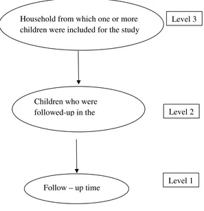
The random effects model or multilevel structure includes correlation among observations within cluster, which in the present study are the households within which more than one child was obtained. Also, each child was followed up for seven time points after baseline. Hence there is correlation between the responses when the same child is followed over a period of time and/or the influence of two or more children sharing the same household environment (77). In random effects model, the residual variance is split into components that pertain to the different levels in the study. The two-level model with the grouping of children within the same household would include the residuals at the household and child level where as the one-level model which includes children with different follow-up time measured with the same child would include the residuals at the child level only (48, 78).

(64)

[image:64.612.182.479.120.427.2]

~ 55 ~ Figure 5.6: Schematic representation of cluster levels:

Figure 5.6 presented above represents the level of hierarchy with the lowest level being the ‘follow-up time’. Each child’s anthropometric measurements were recorded at baseline and every child’s anthropometric measurements were again recorded for seven time points after every six months. Hence the next higher level above follow-up time is ‘child level’. It was possible that if there were children who were in the age groups 5 – 7 years were included even if they belonged to the same household. Hence the next higher level is the ‘household level’. Hence adjustments for the correlation in the responses need to be adjusted at each level. Hence random coefficients model with random intercept and random slope was considered at each level.

Level 3 Household from which one or more

children were included for the study

Children who were

followed-up in the Level 2

(65)

~ 56 ~ 5.6.1 Micro and Macro level units:

The levels which are embedded within another level are also known as ‘micro’ levels where as the upper levels are referred to as ‘macro’ levels. In the present study, the macro level is the household and micro levels are children from the same household and follow-up of each child.

5.6.2 Aggregation:

A common procedure to address if certain risk factors are associated with macro level data is to aggregate the micro-level (lower level) data to macro-level data (higher level).

There can be three errors that happen with aggregation of data. The first potential error is the ‘shifting of meaning’. A variable aggregated to macro level refers to macro unit and not micro units.

The second potential error with aggregation is the ecological fallacy. A correlation between macro-level variables cannot be used to make assertions about micro-level relations.

The third potential error is the neglect of the original data structure, especially when some kind of analysis of covariance is to be used.

5.6.3 The intraclass correlation (ICC):

(66)

~ 57 ~ 5.6.4 Design effect:

It is the ratio of the variance obtained with the given sampling design to the variance obtained for a simple random sample from the same population, supposing that the total sample size is the same. A large design effect implies a relatively large variance. The design effect of a two-stage sample with equal group sizes is given by

Design effect = 1 + (n – 1) g_h.

A relevant model here is the random effect ANOVA model. Indicating by Yij the outcome value observed for micro-unit i within macro-unit j, this model can be expressed as

Yij = µ + Uj + Rij,

Where µ is the population grand mean, Uj is the specific effect of macro unit j, and Rij is the

residual effect from micro-unit i within this macro-unit. In other words, macro-unit j has the ‘true mean’ µ + Uj, and each measurement of a micro-unit within this macro-unit deviates from this true mean by some value, called Rij. Units differ randomly from one another, which is

reflected by the fact that Uj is a random variable and the name ‘random effects model. It is assumed that all variables are independent, the group effects Uj having population mean 0 and

population variance σ2 (the population within-group variance).

The total variance of Yij is then equal to the sum of these two variances, Var(Yij) = τ2 = σ2

The number of micro-units within the j the macro-unit is denoted by nj. The number of macro-units is N, and the total sample size is M =Σj nj.

The intraclass correlation coefficient ρ1 can be defined as

g = ijk+lmi n+Im+op qplrpp s+oIi − jmlt_{uil+k n+Im+op} = v

(67)

~ 58 ~

where, v is the between group or macro units’ variance and wis the within group variance. It is the proportion of variance that is accounted for by the group level.

5.6.5 Within-group and between-group variance:

To disentangle the information contained in the data about the population between-group variance and the population within-group variance, we consider the observed variance between

group and the observed variance within groups. These are defined in the following way. The

mean of macro-unit j is denoted x_. =

e ∑

e

! ,

And the overall mean is x_.. = _z ∑{_!∑ _!e = _z ∑{_! x_.. The observed variance within group j is given by | =

e= ∑ − x.

e

! .

This number will vary from group to group. To have one parameter that expresses the within-group variability for all within-groups jointly, one uses the observed within-within-group variance, or pooled within-group variance. This is a weighted average of the variances within the various

macro-units, defined as |_}'~ = _z={ ∑_!{ ∑ _!e − x_.= _z={ ∑ {_! − 1|.

The expected value of the observed within-group variance is exactly equal to the population within-group variance. For equal group sizes nj, the observed between-group variance is defined

as the variance between the group means,|_'} =

({=) ∑ x.− x.. {

!

For unequal group sizes, the contributions of the various groups need to be weighted

|_'} ₌ 1

( �