Thesis by Or Yogev
In Partial Fulfillment of the Requirements for the Degree of
Doctor of Philosophy
California Institute of Technology Pasadena, California
2009
c 2009 Or Yogev
Acknowledgments The research described in this thesis was conducted in the Engineering Design Research Laboratory at the California Institute of Technology. Many people have been contribute to this research. First, I would like to thank my advisor - Professor Erik K. Antonsson, for his guidance and support along this research, his unbiased enthusiastic and interest in this area, all of which led to great discussions and ideas sharing, which have been matured and demonstrated in this work. I would also would like to thank my coadvisor, Professor Andrew Shapiro for his help and support and his great contribution to this work. Other people which have been part of this research and which I would like to thank are: Professor Rob Philips and Professor Chris Adami.
Abstract
Evolution and development (Evo-Devo), are the two main processes which produce all of the different kinds of phenotypes we see in nature. Evolutionary process is responsible for eliminating the genetic information of weak phenotypes through natural selection, and also for exploring novel genotypes through genetic operations; crossover, mutation. The development process is the process of using the set of rules (codons) written in a genome, to turn a single set (zygote) into a mature phenotype. In this thesis, evolutionary and developmental processes are used to evolve the configu-rations of three-dimensional structuresin silicoto achieve desired performances. Although natural systems utilize the combination of both evolution and development processes to produce remark-able performance and diversity, this approach has not yet been applied extensively to the design of continuous three-dimensional load-supporting structures. Beginning with a single artificial cell containing information analogous to a DNA sequence, a structure is grown according to the rules encoded in the sequence. Each artificial cell in the structure contains the same sequence of growth and development rules, and each artificial cell is an element in a finite element mesh representing the structure of the mature individual. Rule sequences are evolved over many generations through selection and survival of individuals in a population.
Modularity and symmetry are visible in nearly every natural and engineered structure. Under-standing of the evolution and expression of symmetry and modularity is emerging from recent bio-logical research. Initial evidence of these attributes is present in thephenotypesthat are developed from the artificial evolution, although neither characteristic is imposed nor selected for directly.
Contents
Abstract iv
1 Introduction 1
1.1 Definitions . . . 1
1.2 Prior Related Work . . . 2
2 Approach 5 2.1 Material Properties . . . 5
2.2 Evolutionary and Developmental Scheme . . . 6
2.3 Cells . . . 8
2.4 Development Process . . . 8
2.5 Genes/Rules . . . 9
2.5.1 Conditionals . . . 10
2.5.2 Cell-Type Actions . . . 10
2.5.2.1 Cell Division . . . 10
2.5.2.2 Cell Differentiation . . . 11
2.5.2.3 Cell Death . . . 11
2.5.2.4 Cell Adhesion . . . 11
2.5.3 Geometric Actions . . . 13
2.5.3.1 Growth . . . 14
2.5.3.2 Shear . . . 16
2.6 Environment . . . 18
2.7 Genome Structure . . . 19
2.7.1 Syntax Rules . . . 20
2.9 Time Increments . . . 23
2.10 Diseases . . . 24
2.10.1 Repair Process . . . 24
2.11 Maturity . . . 26
2.12 Fitness Evaluation . . . 27
2.12.1 Fitness Description . . . 27
2.12.1.1 Aggregation . . . 28
2.13 Example . . . 30
2.14 Results . . . 32
2.14.1 Phenotype Analysis . . . 33
2.14.2 Development Analysis . . . 34
2.14.3 Genome Analysis . . . 36
2.14.4 Additional Runs . . . 39
2.14.5 Constraints . . . 40
2.14.6 Robustness . . . 40
3 Asynchronous Scheme 43 4 Inhomogeneous Structures under Wind Load 45 4.1 Wind Load . . . 45
4.2 Results, Inhomogeneous Structures under Wind Load . . . 46
5 Robustness 50 5.1 Results . . . 51
5.2 Family of Solutions . . . 52
5.3 Phenotype Robustness . . . 52
5.4 Growth Robustness . . . 53
6 Word Duplication Mechanism, ”WDM” 56 6.1 The Effect of ”WDM” on the Phenotypes . . . 57
6.2 The Relation Between ”WDM” and the Landscape of Solutions . . . 59
6.3 Genes/Word Regulations - ”WDM” and Non-”WDM” . . . 60
6.3.1 Words Distribution in Non-”WDM” . . . 60
6.4 Exploring the Effect of Words on the Phenotype Topology . . . 63
6.5 The Evolution of Simple Modules . . . 68
6.5.1 The Effect of a Nonsymmetric Environment . . . 71
7 SelfRecovery Mechanism 74 8 Appendix 76 8.1 Configuration . . . 76
8.2 Finite Element Scheme . . . 76
8.2.1 Integration scheme . . . 81
8.2.2 Assembly scheme . . . 81
9 Cell Adhesion Scheme 83 9.1 Cell Adhesion Scheme in Finite Element Mesh . . . 83
9.2 Overview of Existing Mesh Techniques . . . 84
9.2.1 Our Approach . . . 85
9.2.2 Overview . . . 85
9.3 The Adhesion Approach . . . 85
9.4 Hexahedral Linear Brick Element . . . 89
9.5 The Conjugate Gradient Method . . . 93
9.6 Results . . . 96
9.7 Application . . . 97
9.8 Conclusions . . . 101
9.9 Future Work . . . 103
List of Figures
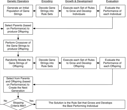
2.1 The computational evolutionary development process. . . 7
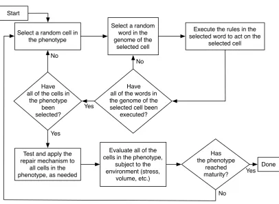
2.2 The growth and development process. . . 8
2.3 The basic structural hexahedral “brick” three dimensional finite element. . . 9
2.4 Celldivision operation. . . 11
2.5 Adhesion process . . . 12
2.6 The four basic geometric operations observed in sub-regions of plants. . . 13
2.7 Hexahedral mesh vs grid mesh . . . 14
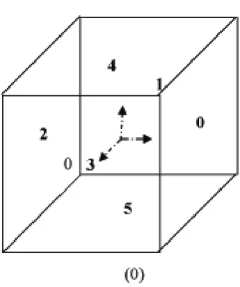
2.8 Face numbering - Local configuration. . . 15
2.9 Shear operation. . . 17
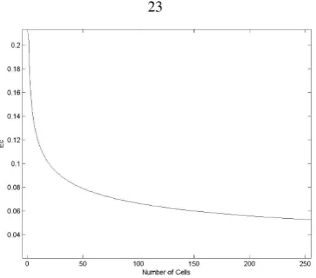
2.10 The amount of energyEc available to each cell during growth, as a function of the total number of cells in the growing phenotype. . . 23
2.11 The average usage of the repair mechanism. . . 25
2.12 The average usage of the repair mechanism with respect to time for one phenotype during the growth and development process. . . 25
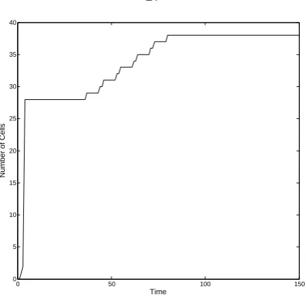
2.13 A typical development process. . . 27
2.14 A representative preference function. . . 29
2.15 A simple reference solution. . . 31
2.16 Initial setting of the growth process . . . 31
2.17 The evolution of fitness values with respect to the number of generations . . . 32
2.18 The evolution of fitness values once the phenotype has reached the desired height. . . 33
2.19 Three stages of an early evolved phenotype . . . 34
2.20 Two views of a first phenotype (fitness value = 2.11), which is able to support the load, as indicated by the predominantly green color of the cells. . . 35
2.22 Six stages in the growth and development of the phenotype shown in Figure 4.2. . . 37
2.23 Four different phenotypes, growing from the same genome . . . 38
2.24 The distribution of fitness values of phenotypes grown and developed from a single genotype. . . 38
2.25 The genome for the phenotype shown in figures 4.2 and 2.22 contains 9 different words. 39 2.26 Maximum mechanical stress, normalized to the material yield stress (σ/σy) vs. angle of the load vector. . . 41
2.27 Fitness value vs. angle of the load vector. . . 41
2.28 An evolved phenotype which has been generated by additional simulation. . . 42
4.1 four different view of an inhomogeneous phenotype . . . 47
4.2 four different view of an inhomogeneous phenotype . . . 48
4.3 Growth process of the phenotype in Figure 4.1. . . 49
5.1 Three different phenotypes from three different stochastic environment experiments (SEE). . . 51
5.2 Phenotype evolved with an unvarying load (fixed environment). . . 53
5.3 A comparison between two evolutionary process . . . 54
5.4 A comparison between the standard deviation of two evolutionary process . . . 54
5.5 Fitness distribution of two genomes. . . 55
6.1 ”Best” phenotype from both experiments . . . 58
6.2 A convergence comparison of both experiments. . . 58
6.3 The evolution of new words during evolution. . . 59
6.4 Non-”WDM”, the distribution of words expression. . . 62
6.5 The evolution of new words during evolution. . . 62
6.6 ”WDM”,the distribution of words expression. . . 64
6.7 ”WDM”, repeated times in the genome vs number of executions . . . 66
6.8 The effect of word elimination on the fitness distribution. . . 68
6.9 Phenotype resulting from word elimination . . . 69
6.10 Six stages in the growth and development of the ’tripod’ phenotype . . . 70
6.11 The first primitive phenotype, contains word9. . . 71
7.1 Six stages during the growth of a selfrecovered phenotype. . . 75
8.1 The local-global mapping. . . 77
8.2 The basic structural hexahedral “brick” 3-D finite element. . . 78
9.1 Adhesion process . . . 86
9.2 Pseudocode outline of the algorithm. . . 97
9.3 Example 1 . . . 98
9.4 Example 2 . . . 99
9.5 Example 3 . . . 100
Nomenclature
V0 initial volume of the cell
h height of a selected cell face
Ap area of a selected cell face
R, S, T coordinates of a point inside a cell in local coordinates
r, s, t coordinates of a point inside a cell in reference coordinates
F deformation tensor
r a vector form ofr, s, t
R a vector form ofR, S, T
α a scalar which represents change in volume
v cell volume after applying geometrical operation
V cell volume before applying geometrical operation
J jacobian
Ni interpolation function
Yi the Y node i coordinates on the reference configuration
Zi the Z node i coordinates on the reference configuration
dR, dS, dT infinitesimal material vectors in the X,Y and Z direction respectively.
a directional vector originating in the reference configuration
κ1 first coefficient for the shearing operation
κ2 second coefficient for the shearing operation
α1, α2, α3 expansion coefficients
σ Cauchy-Green tensor
s morphogen diffusion rate
d morphogen diffusion constant
Ec energy consumption
Bc metabolic rate
S total volume of the phenotype
Nc number of cells comprising the phenotype
k node number
x(mk) vector coordinate of thekthnode
m dummy index
αm deformation measure of a node, used as part of the repair process
xm node coordinates in the present configuration, use as part of the repair process
f0 the total deformation level of the phenotype
gm degree of deformation of the cell
xm,k node coordinates, used in the process of computingf0 x node coordinates
Jm Vector, used in the process of computingf0 µi preference function for theithvariable
Si theithperformance variable
a,b preference function parameters
α slope parameter for preference functions
ωi importance weight for aggregation Ps aggregation function
s degree of compensation for aggregation
Chapter 1
Introduction
Natural evolution has produced systems of fantastic complexity, robustness and adaptability. Recent research has shown that it is the combination of both evolution and development processes that has produced these remarkable results [1, 2]. Evolution does not act directly on the configura-tions of adult phenotypes, rather it successively alters and revises therulesthat guide the growth of a zygote into an embryo and its further development into an adult.
The computational evolutionary development approach presented here is based on an artificial evolution using indirect encoding of growth and development rules. The approach was tested on a classical structural engineering problem. The results demonstrate that artificial evolution and embryogenesis can synthesize phenotypes with novel configurations that exhibit modularity, and which meet performance goals.
The objective of this research is not simply to evolve structures that meet the desired perfor-mance requirements, but also to explore complex design environments (including functionally-graded, tailored composite materials) and to develop a fundamental understanding of the origin and development of modularity in design, and the design rules that give rise to modular design configurations.
1.1
Definitions
Phenotypesare
the set of observable characteristics of an individual resulting from the interaction
of its genotype with the environment”.
the production of proteins using transcription factors, and hence the growth and development of the organism. The genome contains the set of instructions for the development process while the environment provides inputs that regulate the instructions [3].
Natural evolutionary processes refine the sets of rules, in the form of genes, which result in adult forms. Natural selection acts upon the phenotypes, thus rewarding sets of rules that produce fit individuals. The indirect character of the encoding of genetic information in natural systems, and the inter-relationship between evolution of rules and the growth and development of adult forms, has been responsible for the diversity, complexity, modularity, robustness, and adaptability in the natural world [4, 5].
EmbryogenyorEmbryogenesis is the process of growth by which a genotype develops into a phenotype, and is central to the emerging understanding of the relationship between evolution and development.“It should be noted that the correct term isembryogeny, which refers to the process, rather than the oft-misused termembryology, which refers to the science of studying embryos and embryogenies.” [6]
1.2
Prior Related Work
Artificial evolution, in the form of Genetic Algorithms (GA), has been used in a wide variety of application areas [10, 11, 12, 13]. The goal of this prior work has been to improve one or more features of a problem, and GA’s have been applied in a wide variety of application areas. The key element of GA’s, first stated by Holland [14], isimplicit parallelism. The idea is that the GA scheme of actions; selection, crossover and mutation performed on N individuals, implicitly searches for an optimum in N3 space. This result is powerful, since it enables the rapid exploration of large solution spaces.
The majority of optimization problems that make use of the genetic algorithm approach have employeddirectencoding. In direct encoding, there is a one-to-one relationship between the genetic information in an individual and the configuration of the individual. Most commonly, the genetic information contains a description of the individual, in contrast with indirect encoding, where the genetic information contains a set of rules that, when executed (and perhaps influenced by various environmental factors), guide the growth and development of a single cell into an adult.
evo-lution. Traditional structural evolutionary methods generally start by generating a fixed mesh grid (like a chess board) with a predefined volume and constraints, such as external forces and bound-ary conditions [15]. Every cell in the grid can have one of two states, either material is present or absent. The genetic information in this approach contains information indicating the material state in each cell of the grid. Once the initial configuration and the boundary conditions are defined (loads, constraints,etc.), an evolutionary process searches for the configuration exhibiting the best performance. This is an evolution using adirectencoding, with no embryogeny, and thus there is a one-to-one mapping between the genotype and phenotype, resulting in an optimization problem with a large but finite number of possible states [16]. This method produces structures that reflect the underlying shape of the grid [10] and is not able to create continuous or smooth structures. These grid-based building-block structures are not only unrealistic from an engineering perspective, but from a mathematical point of view they search in a limited solution space, resulting in local optima. Indirect encoding, and the study of artificial embryogeny, has been proposed previously [6, 17, 18, 19]. In most examples the goal has been to grow and evolve a predefined target shape on a predefined grid starting from a single cell, using simple rules such as cell division and protein diffusion. Early work in this area has demonstrated the ability of indirect encoding to produce modular phenotypes in graphs and patterns [20, 21, 22].
ar-tificial evolutionary and development system [15]. In his system cells were created with a set of genes that were to be evolved into a desired 3D shape in response to the concentration field of a morphogen [29, 30, 31, 32, 18, 20].
Chapter 2
Approach
In the work reported here, an artificial embryogeny has been created for structures. The two critical foundational elements of this work are the selection of the artificial cell (the basic structural element), a collection of which constitute each individual, and the artificial genes (the rules) which are evolved into the genetic information for each individual.
The genetic information of an individual is shared by all of its cells. Each individual cell exe-cutes its rules until a mature structure is formed. Once maturity is reached, an evaluation scheme determines the fitness (performance) of the structure. Evolutionary operations (selection, crossover, and mutation) alter and refine the genetic information in a population of individuals over multiple generations. The results are structures that meet the desired performance goals.
2.1
Material Properties
One of the main advantages of the approach presented here is the ability to evolve inhomoge-neous structures with a high degree of internal complexity. It has been observed that the materials properties of biological structures are unique and complex. A wide range of stiffnesses and strength are exhibited, and in many cases a combination of a high degree of compliance with high strength produces robust structures that are difficult or impossible to replicate with the engineered materials of today. One contributing factor to this difference is inhomogeneity: the material properties of many natural structures change from location to location.
have not yet been developed.
2.2
Evolutionary and Developmental Scheme
The evolutionary and developmental scheme used here is derived from a genetic algorithm, and is illustrated in figure 2.1. The growth and development process in particular is shown in figure 2.2. The algorithm is initialized with sets of randomly generated genomes. Development begins with a single artificial cell. This cell is placed on (and attached to) a ground plane. A load vector, to be supported by the evolved and developed structure, is positioned above the initial cell. The origin of the load vector radiates a signal, analogous to a morphogen. The goal is for individuals comprising one or more cells to grow to reach the height of the morphogen and to be able to support the load.
One individual is grown from each genome, by executing the rules in the genome. Once each individual reaches maturity, its fitness is evaluated by means of a finite element analysis and addi-tional parameters. The selection process is based on theroulette wheel method, where the fitness values of each individual are used to select parents to produce offspring, where a higher fitness value results in a higher probability of being selected for reproduction.
Once two parents have been selected, they produce offspring through a crossover process. In this process, the genome from each parent is cut at a randomly selected word boundary, where a word is a sequence of rules. One portion of the gene string from each parent is joined together producing a child. The remaining gene strings from each parent are joined together producing a second child.
Similar to evolution in nature, the genome is also subject to random mutation. The mutation process can erase an entire word and replace it with another, or replace a single rule within a word. These three steps: selection, crossover and mutation are repeated, and each repetition is defined as one generation.
Execute each Set of Rules to Grow and Develop
Individuals
Evaluate the Performance of each Individual
Select Parents (based on Performance) to
produce Offspring
Perform Crossover of the Gene Strings to
produce Offspring
Randomly Mutate the Gene Strings of
Offspring
Evaluate the Performance of
each Offspring
Select from Parents and Offspring (based
on Performance) to Create the Next
Generation
Stopping Criteria Met?
The Solution is the Rule Set that Grows and Develops the Best Performing Individual
No Yes
Generate an Initial Population of Gene
Strings
Execute each Set of Rules to Grow and Develop
Offspring
Genetic Operators Growth & Development Evaluation
Decode Gene Strings into
Rule Sets Encoding
Decode Gene Strings into
[image:20.595.120.535.203.562.2]Rule Sets
Execute the rules in the selected word to act on the
selected cell No
Yes Select a random cell in
the phenotype
Select a random word in the genome of the
selected cell
Test and apply the repair mechanism to
all cells in the phenotype, as needed
Evaluate all of the cells in the phenotype,
subject to the environment (stress,
volume, etc.) Have all of the words in the genome of the selected cell been
executed? Have
[image:21.595.121.528.66.362.2]all of the cells in the phenotype been selected? Has the phenotype reached maturity? No Yes No Done Yes Start
Figure 2.2: The growth and development process.
2.3
Cells
The model begins with a structural element that is analogous to a cell in biology. Cells in nature act as building blocks for organisms [74]. The basic structural element in the approach presented here is an extended 3-D triclinic hexahedral finite element “brick”, illustrated in Figure 2.3. Each cell-like finite element contains an identical copy of the genetic information of the individual. A collection of cells forms a finite element mesh, which defines the phenotype.
2.4
Development Process
Figure 2.3: The basic structural hexahedral “brick” three dimensional finite element.
are also subjected to the global environment (gravity and the morphogen concentration) and their local environment (stresses and signals from nearby cells). Because the environment of each cell is different, the regulation mechanisms may cause different rules in different cells to be executed. This repeated process of cell production and rule/gene regulation creates a phenotype which will eventually grow and reach the load morphogen. Once a phenotype has reached the load, the load is applied to the top cells that coincide with the morphogen. This load generates a mechanical stress distribution along the phenotype which will alter the local environment on the cells, and may cause the rule/gene regulation mechanisms to alter the further growth and development of the cells. The process of evaluating the mechanical stresses on the cells at each time step is performed by solving a finite element scheme.
2.5
Genes/Rules
Rules are the basic instructions encoded inside the genome. Here, rules dictate the growth and development processes of each cell of the phenotype. Mimicking nature, the basic structure of genetic information is anif-conditionalthen-action rule.
Two main principles guided the creation of the rule elements (conditionals and actions) to form genes. The first principle was to create conditional rules that respond only to the local environment of the cell. The second principle was to choose action rules that will not put any constraint on the topology of the phenotype and can generally develop any 3D shape.
phenotypes.
The rules used here fall into three groups: geometric actions and cell-type actions, and condi-tionals in the form of veto tests. Geometric rules represent instructions which have an effect on the shape of the cell. Cell-type rules alter the type of the cell, and therefore mimic basic process ob-served in cell biology. Veto tests affect other instructions at the genome level, and will be discussed first.
2.5.1 Conditionals
Conditional artificial rules are “veto” or “suppression” rules. These rules affect other rules only at the genome level, by turning actions off or on according to whether the conditional test is satisfied or not. Veto genes that switch regulatory mechanisms on or off have been observed in biology [1]. For example tumor suppression genes that turn off other genes that produce tumor cells [36].
2.5.2 Cell-Type Actions
Cell-type rules are actions which mimic basic operations in cell biology. Four basic opera-tions are used here: cell division, cell differentiation, cell death, and cell adhesion. Each of these operations was modeled as a single rule.
2.5.2.1 Cell Division
The cell division rule is responsible for creating new mass and thus generates more building blocks (new cells) for the construction of the phenotype. Cells divide with respect to a given vector in the reference configuration of the cell. The vector specifies a face of the new cell. The selection of the face uses the inverse isoparametric mapping [37], and is performed by translating the vector into the cell center point and then determining the face which intersects the translated vector. Once the face has been determined, a new triclinic hexahedral cell is created perpendicular to the selected face, such that the total volume of both cells equals the volume of the parent cell prior to division, as shown in figure 2.4.V0is defined as the initial volume of the cell prior to division. An isotropic
shrink operation is applied with parameterα = q3 1
2. This operation will shrink the cell into half
Before Division After Division
Figure 2.4: Celldivision operation.
h= V0 2Ap
(2.1)
A cell will attempt to divide, prioritized according to the parameters governing the rules in its genome.
2.5.2.2 Cell Differentiation
Two different kinds of cells are modeled, one made of steel and the other made of aluminum. The cell differentiation rule simply alters the material properties of a cell from one type to the other.
2.5.2.3 Cell Death
Cell death is a self extermination mechanism, which kills the cell and removes it from the phenotype, and from further consideration in the embryogeny computations.
2.5.2.4 Cell Adhesion
During growth, two cells may intersect, causing them to adhere. In nature, this fundamental process creates the integrated structures forming the configuration of the organism. Studies have shown that the speed of the adhesion process is short [38]. Adhesion of nearby cells is modeled in a manner similar to the adherence of bubbles [39].
a
b
[image:25.595.173.477.88.658.2]c
Isotropic growth Anisotropic growth
[image:26.595.211.436.53.308.2]Shear Rotation
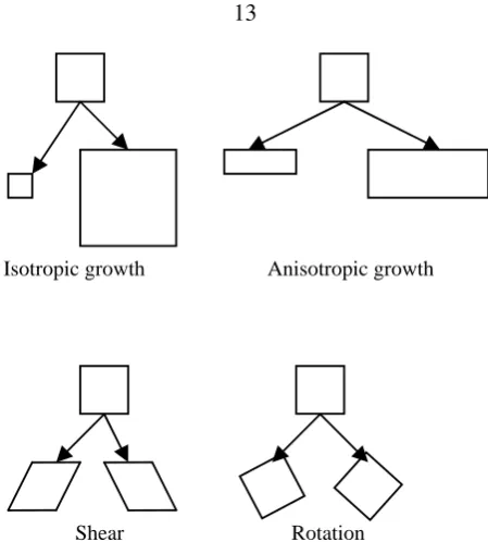
Figure 2.6: The four basic geometric operations observed in sub-regions of plants.
Three major steps are executed during the cell adhesion process; first determine the correspond-ing faces to be adhered; second determine the pairs of nodes to be merged, and third optimize the positions of the merged nodes, as shown in figure 9.1.
A detailed explanation of the adhesion process can be found in appendix 9.
2.5.3 Geometric Actions
The idea of formalizing the geometrical rules arises from studies of the development processes of plants. Plants are remarkable engineering structures that sustain high dynamic loads, for example, those generated by wind. The topological structure of plants and their material complexity provide them with the ability to sustain high mechanical stresses. During the natural embryogeny of plants, every 3D region (which is a collection of several cells) can deform according to nine different geometric operations: one for isotropic growth, two for anisotropic growth, three for shear and three for rotation [40], illustrated in figure 2.6. Every cell in the model presented here represents a 3D region that can be deformed according to these geometrical operations. Every geometric operation, excluding rotation, corresponds to a geometric rule.
Fig-a b
Figure 2.7: (a) 3D hexahedral linearlly conformal mesh [41]. (b) 3D rectilinear grid mesh [42].
ure 2.7b. Even a simple arc has a crude representation in the fixed mesh-grid approach.
The action of a geometrical rule is always applied in the reference configuration. Since there is a one-to-one mapping between the local and the reference configuration, it will be more conve-nient to execute the geometrical operations locally and then map the result back to the reference configuration. In order to be consistent with the next derivations, the faces of the cell in the local configuration have been numbered according to Figure 2.8.
2.5.3.1 Growth
The action of this rule is to expand the cell by an amount in all directions. Assuming the cell is in the local configuration, as shown in Figure 2.3, the following mapping is defined by equation 2.2. Every pointR, S, T, corresponding to a point inside the cell before applying the geometrical rule, is mapped to a pointr, s, tafter the geometrical rule has been applied. Both points are defined in the coordinate system of the local configuration.
r =α1R ; s=α2S ; t=α3T (2.2)
The coefficientsα1, α2, α3representing the expansions along each of the three orthogonal axes.
Whenα1=α2 =α3, the growth is isotropic.
The deformation gradient tensor for this mapping is defined in equation 2.3.
F= ∂r
∂R =
α1 α2
α3
Figure 2.8: Face numbering - Local configuration.
The volume change of any infinitesimal point dV todv can be computed according to equa-tion 2.4.
dv
dV = det (F) =α1α2α3 (2.4)
Using equation 2.4, the volume change of the entire cell can be computed according to equa-tion 2.5.
vcell
Vcell
=J= det (F) =α1α2α3 (2.5)
The mapping in equation 2.2 is applied to the nodes of the cell in the local configuration. Since the mapping is homogeneous, mapping the nodes will set the map of the entire cell. By settingα
and applying this mapping, the change in volume of a cell in the local configuration will beα1α2α3.
DefineV˜ to be the volume of the cell in the reference configuration prior to this mapping. A unit volume1of the cell in its reference configuration prior to the application of this mapping is given in equation 2.6. The quantitiesR,S,Tare defined as material fibers in the local configuration.
dV˜ =Ni(dR)Xi×Ni(dS)Yi×Ni(dT)Zi (2.6) 1
A unit volume of the cell in its reference configuration, after this mapping has been applied, is given in equation 2.7, wherer,s,tare material fibers in the local configuration after the mapping has been applied.
d˜v=Ni(dr)Xi×Ni(ds)Yi×Ni(dt)Zi (2.7) Again using the definition of the gradient deformation tensorFshown in equation 2.3, equation 2.7 can be written in a new form, shown in equation 2.8.
dv˜=Ni(FdR)Xi×Ni(FdS)Yi×Ni(FdT)Zi (2.8)
SinceNiis a linear operator, equation 2.8 can be rewritten into the form of equation 2.9.
dv˜ = FNi(dR)Xi×FNi(dS)Yi×FNi(dT)Zi = JNi(dR)Xi×Ni(dS)Yi×Ni(dT)Zi =JdV˜
(2.9)
The volume ratio of the cells in the reference configuration, after the mapping in equation 2.2 has been applied, is equal to the volume ratio of the cells in the local configuration, after the mapping in equation 2.2 has been applied. This conclusion enables the growth operation to be applied in the local configuration of the cell.
2.5.3.2 Shear
(1 2 ,1,1 2+ κ1 + κ2)
a
(1,-1,1)
Figure 2.9: Shear operation.
The second step is to deform the cell in the local configuration such that the edges which are perpendicular to the selected face become parallel to a, as shown in figure 2.9. The mapping, defined in equation( 2.10) shears the cell in a predetermined direction such that the volume of the cell remains the same. The number below each box in equation 2.10 corresponds to a particular face with respect to the notation defined in Figure 2.8.
r=R+κ1(S+ 1) s=S
t=T +κ2(S+ 1)
r=R+κ1(T−1) s=S+κ2(T −1) t=T
r =R
s=S+κ1(S−1) t=T+κ2(S−1)
1 2 3
r =R+κ1(T + 1) s=S+κ2(T + 1) t=T
r =R+κ1(S+ 1) s=S
t=T+κ2(S+ 1)
r =R+κ1(S−1) s=S
t=T+κ2(S−1)
4 5 6
(2.10)
It is easy to show that each of the mappings in equation 2.10 is isochoric (volume preserving), by following the same derivation as in equations 2.3, 2.4, and 2.5.
The relation between the coefficientsκ1, κ2 and the target direction vectora ={a1, a2, a3}is
κ1 = √ a2 1−a2
2−a23
κ2 = √ a3 1−a2
2−a23
κ1= √ −a1 1−a2
1−a22
κ2= √ −a2 1−a2
1−a22
κ1 = √ −a2 1−a2
2−a23
κ2 = √ −a3 1−a2
2−a23
1 2 3
κ1 = √ a1 1−a2
1−a22
κ2 = √ a2 1−a2
1−a22
κ1= √ a1 1−a2
1−a23
κ2= √ a3 1−a2
1−a23
κ1 = √ −a1 1−a2
1−a23
κ2 = √ −a3 1−a2
1−a23
4 5 6
(2.11)
2.6
Environment
The environment in which the individuals are grown contains factors which every cell can sense, and which can affect the way rules are expressed. The environment can trigger the execution of rules and control their expression. Biologists studying growth and development have found that the concentration of morphogens [43] and mechanical stresses [44] are two crucial factors which influence the growth of a phenotype. Various mathematical models illuminate the role the two effects play in determining the size and shape of tissues [45, 46]. In natural systems, information from the environment is transferred to the cells through proteins known as receptors. The receptors transfer the information by generating chemicals that diffuse through the cell membrane at some level of concentration. This concentration stimulates the action of rules at the local cell level during the developmental stage.
In the simulated evolutionary embryogenesis here, as well as in nature, the relationship between the information that cells receive from the environment and the development of the phenotype is not predetermined. Rather, conditionalsare available to the evolutionary process that sense the concentration or gradient of each morphogen. In this way, the evolutionary process establishes the relationship between information and growth and development.
The morphogens represent points, surfaces or volumes in space, with associated engineering requirements. In the artificial embryogeny presented here, two kinds of morphogens are present. The first morphogen represents an external load to be supported by the phenotype. The morphogen is located at a predetermined point and produces a chemical which continuously diffuses in space according to equation 2.12. The parametersrepresents the concentration of the morphogen, whiled
which cells adhere when they intersect the surface.
s=e−d (2.12)
The phenotype is subjected to gravity effects and an external load. These two effects generate internal mechanical stresses within the cells, which can be represented by the Cauchy-Green tensor given in equation 2.13.
σ=
σxx σxy σxz
σxy σyy σyz
σxz σyz σzz
(2.13)
By solving a finite element scheme at every time step, the mechanical stress distribution within the cells can be calculated [37]. There are six independent parameters which can be derived from the Cauchy stress tensor and added as environmental factors. The parameters are: the three principal values and the three principal directions of the Cauchy stress tensor. Since every point inside the cell has a different stress tensor, only the point which has the maximum principal stress is considered. The calculations are outlined in appendix 8.2.
Two additional environmental factors correspond to the volume and the age of the cell. The volume of a cell is simply the value of the Jacobian, defined in equation( 8.2.7) in appendix 8.2. The age of the cell corresponds to the number of time steps that have passed since the cell was created. Cells also maintain information about their distance from neighboring cells. This information is used to trigger the execution of the cell adhesion rule.
2.7
Genome Structure
Table 2.1: Geometric Rules
ID Name N Optional Parameters
A Shear 1 (d,e,f,h)×fractional coefficient B Anisotropic 3 (a,b,c,g,i)×fractional coefficient
growth
C Isotropic 1 (a,b,c,g,i)×fractional coefficient growth
S Isotropic shrink 1 (a,b,c,g,i)×fractional coefficient
N =number of parameters
2.7.1 Syntax Rules
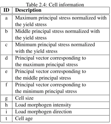
Every rule comprises one capital letter and several lower case letters, each with a fractional coefficient. The capital letter identifies the type of a rule. The lower case letters correspond to the environmental factors which guide the action of the rule within the cell. The fractional coefficient is a number between 0 and 100 which represents the level of expression of the rule with respect to the environmental factor that follows it (a mechanism analogous to transcription factors in nature). Tables 2.1, 2.2, and 2.3 contain four columns, the first column corresponds to the identifying let-ter, and the second column corresponds to the name of the rule. The third column specifies how many additional parameters each rule has while the fourth column specifies the type of additional parameters, as listed in Table 2.4.
The rule execution process begins by reading the identifying letter of the rule, followed by a set of environmental factors each with its fractional coefficient. Each environmental factor is normalized to a nominal value.
aim of the normalization process is to equally scale all of the factors. The following normal-ization are used here: the mechanical stress is normalized to the yield stress of the material, the volume of the cell is normalized to the initial volume of the first cell, the intensity of the mor-phogen is normalized with the mormor-phogen intensity impinging on the first cell at the initiation of the growth process. at the first time step, and the age of the cell is normalized with the maximum age allowed. The product of the environmental factor and the fractional coefficient specifies the level of expression of the rule. For instance, the set of letters S30g reduces the volume of the cell by 30 percent.
Table 2.2: Cell-Type Operations
ID Name N Optional Parameters
D Cell division U (d,e,f,h)
K Cell death 0 none
F Cell differentiation 0 none
N =number of parameters U=Unlimited number
Table 2.3: Veto (conditional) operations
ID Name N Optional Parameters
V Suppress below 1 (a,b,c,g,i)×fractional coefficient W Suppress above 1 (a,b,c,g,i)×fractional coefficient
[image:34.595.211.439.435.690.2]N =number of parameters
Table 2.4: Cell information
ID Description
a Maximum principal stress normalized with the yield stress
b Middle principal stress normalized with the yield stress
c Minimum principal stress normalized with the yield stress
d Principal vector corresponding to the maximum principal stress e Principal vector corresponding to
the middle principal stress f Principal vector corresponding to
the minimum principal stress g Cell size
2.8
Metabolism and Thermodynamics
A thermodynamic energy model which balances the energy required to maintain the organism mass with the energy required to create a new mass [47], is incorporated in the growth and develop-ment process used here. The amount of energyEc that each cell consumes in a given time step, is proportional to its metabolic rateBc. Part of this energy is used for maintaining the existing pheno-type while the remaining energy may be used for creating new mass, as shown in equation 2.14.
Ec =E0Bc∆t (2.14)
Using Kleiber’s Law [48, 49], and assuming small variation in the volume of the cells( Small variation of the volume of cells is a requirement in the fitness function), the metabolic rate Bc of each cell is proportional to the size of the phenotypeS(the total volume of the phenotype) divided by the number of cells, Nc, as shown in equation 2.15. The parameter E0 is a proportionality
constant which sets the energy scale.
Bc ∝
S3/4 Nc
(2.15)
By combining equations 2.14 and 2.15, and by settingE0 = 1, a thermodynamic size limit can
be specified for the phenotypes, as shown in equation 2.16. At the beginning of every time step, each cell contains an amount of energyEc. This energy is utilized by the cell to execute its genome. Every rule (operation) may consume a different amount of energy.
Ec =
S3/4 Nc
(2.16)
The following scheme addresses the process of assigning energies to rules. First, consider a scenario where there is non-stop equally sized cell production. Assuming E0 = 1, Ec can be plotted, as shown in figure 2.10. The total amount of energy,Ec, is reduced as the number of cells increases since the volume of the phenotype increases. Setting the energy consumption of the cell-division rule to be aboveEc(N), forces a weak upper limit to the size of the phenotype. All the other energies are set to be less than the division energy. This enables the phenotype to change its topology without adding new mass.
Figure 2.10: The amount of energyEcavailable to each cell during growth, as a function of the total number of cells in the growing phenotype.
approach will permit new mass to be created at the expense of removing existing mass. This po-tentially changes the topology of the phenotype. However, the thermodynamic balance will not prevent phenomena such as unlimited cell division or extermination of the entire phenotype. These last phenomena are addressed by evolution and disease mechanisms.
2.9
Time Increments
The growth and development processes in nature proceed continuously. In order to simulate these processes numerically, a time step has been defined. A time step starts when the first cell executes its first rule and ends when the last cell executes its last rule.
2.10
Diseases
Individuals may suffer from a disease during growth and development. A disease only occurs as a consequence of a defective genome, and diseases adversely affect the growth process of the phenotype. When a developmental disease is detected in an individual, a penalty is applied to the measure of its performance. The following diseases are present.
High cell division rate : an upper limit to the number of divisions at one time step is set. If the number of cell divisions exceeds the threshold value, it is identified as a disease.
Self extermination : A defective genome might contain instructions that will eliminate all of the cells in that phenotype at some point during its development. This is identified as a disease.
Morphology of the cell : As part of the repair process (which is a subprocess of the growth and development process illustrated in Figure 2.2) every cell is regularly tested with equations 2.17 and 2.19 to determine whether it is “tangled” or highly deformed. An automatic repair mechanism (which is described in the following section) attempts to fix any cell that exceeds threshold values. If the repair mechanism fails to repair the cell, then the growth process is stopped. The phenotype is then evaluated, and a performance measure is assigned to the phenotype based on its current state. Since the phenotype fails to reach maturity, the performance measure is penalized (reduced by a factor). This process produces a comparative benefit for individuals that reach maturity, but will not eliminate phenotypes that have good properties but fail to reach maturity.
2.10.1 Repair Process
Figure 2.11: The average usage of the repair mechanism.
Figure 2.12: The average usage of the repair mechanism with respect to time for one phenotype during the growth and development process.
to these changes. Figure 2.11 shows the average usage of the repair mechanism during the process of evolution. The average usage is defined as the total number of times the repair mechanism is used by all cells through all of the time steps for the phenotype to reach maturity, divided by the sum of the number of cells in the phenotype at each time step. The use of the repair mechanism generally decreases in the beginning evolutionary process. Figure 2.12 shows the utilization of the repair mechanism during the growth process of one phenotype. Theyaxis represents the average use of the repair mechanism with respect to the cells. On average, 1.27 cells were repaired at each time step.
equation 2.17, wherex(1)m ,x(2)m ,x(3)m correspond to the coordinates of three nodes which are adjacent to nodex(0)m , wheremis a dummy index, and a negative value ofαmcorresponds to a tangled node which needs to be untangled. The untangling process is performed using the conjugate gradient method with a global function that is to be minimized defined in equation 2.18. This process is described in detail in [53].
αm=
x(1)m −x(0)m ×x(2)m −x(0)m ×x(3)m −x(0)m (2.17)
f0 =
1 2
M
X
m=1
{|αm| −αm} (2.18)
The second restriction corresponds to deformation level. A conditional number,gm, is defined in equation 2.19, wherexm,kare the adjacent coordinates to nodex,gm ≥1.
em,k = xm,k−x
Jm = [em,1, em,2, em,3]
gm = det
J
T mJm
(2.19)
The value of gm represents the degree of deformation of the cell. A high conditional number corresponds to a highly deformed cell that needs repair. The repairing mechanism is to minimize the objective functionf0 defined in equation 2.20, whereαm is defined in equation 2.17. Further details may be found in [52].
f0 =|Jm| |Adj(Jm)|/|αm| (2.20) Each of the repair processes is an iterative optimization process. If either process fails to con-verge after a large number of iterations, a disease will be identified
2.11
Maturity
0 50 100 150 0
5 10 15 20 25 30 35 40
Time
[image:40.595.212.436.62.282.2]Number of Cells
Figure 2.13: A typical development process.
of stable size.
Figure 2.13 shows a typical growth process of a representative phenotype. The y-axis marks the number of cells in the phenotype while thex-axis represents the development time. During the initial stage of the growth process, the production rate of new cells is relatively high. As time evolves, this rate decreases and stabilizes. There are two stabilization regions (plateaus) in which no new mass is created. The first plateau is unstable since the phenotype continues to produce new mass after some time. The second plateau is stable. The phenotype has reached stability such that no additional mass is created.
2.12
Fitness Evaluation
2.12.1 Fitness Description
cells intersects with the location of the source of a morphogen then this distance is zero. The age of the phenotype corresponds to the number of time steps a particular individual has been growing without developing a disease. The parameter that establishes the maximum volume of a single cell puts constraints on the size of the individual cells, preventing extremely large cells in the phenotype.
2.12.1.1 Aggregation
In order to establish the fitness of individuals in the population, two approaches have been used here: aggregation of the multiple values into a single scalar [55, 56], and the Pareto optimization method [57]. In both cases, the objective is to minimize the fitness value(s).
The aggregation approach builds on prior engineering design work of Scott and Antonsson [58], where both importance weighting and degree of compensation among the variables are utilized. The degree of compensation specifies how a strong value of a particular performance variable may compensate for a deficiency of another variable.
To begin, the value of each performance variable is mapped to a preference value between 0 and 1 by a preference function, where a preference value of 1 corresponds to a perfectly acceptable value of the performance variable; a preference of 0 corresponds to a completely unacceptable value of the performance variable. A preference functionµi, maps every variableSito a value on the real interval line[0,1]using equation 2.21, as illustrated in Figure 2.14. The variablearepresents the value such that any value below it will be considered to have a preference value of 1. The variable
brepresents the maximum value such that any value above will be considered to have a preference value of 0. Settingaandbcontrols the range of feasible solutions and also provides the ability to put constraints on the phenotype.
The slope of the function specifies the improvement rate which corresponds to a particular vari-able. One of the major concerns which must be taken into account in choosing the preference function corresponds to the volatility of the individuals within the population. A single mutation in the genome may turn an individual with high performance into a non feasible one. While this phe-nomena provides the ability to explore a large span of the space of possible solutions, its drawback is that it significantly penalizes individuals with poor performance. This phenomena of poor behav-ior is often observed at the early stages of the evolutionary process where most of the population has low measures of performance.
1
0
b
a Crisp set
Figure 2.14: A representative preference function.
a preference mapping in the form of an exponentially decaying function, shown in equation 2.22, whereαsets the slope. By reducing the value ofα, the preference corresponding to the variableb
is increased. The value ofbcan be increased such that a wider range of values will be considered and thus, individuals that are poorly performing can be distinguished.
µi :Si→[0,1] (2.21)
µi =
1 Si< a
e−α(Si−m) a≤S
i < b
ε Si≥b
(2.22)
Once all the preference functions have been defined, the weight and the degree of compensa-tion of these values are used in the relacompensa-tion 2.23. The weight for theµi performance variable is represented byωi, andsrepresents the degree of compensation. Observing equation 2.23, it can be seen [58] thats = 1corresponds to a weighted sum, thelims → 0 corresponds to the weighted product (µω11 µω22 . . . µωn
n ) 1
ω1+ω2+...+ωn, and lims → −∞ corresponds to min (µ
1, µ2, . . . , µn). Here, only compensation valuess≤0are used.
Ps((µ1, ω1),(µ2, ω2), . . . ,(µn, ωn)) =
ω
1µs1+ω2µ2s+. . .+ωnµsn
ω1+ω2+. . .+ωn
1s
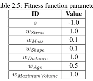
Table 2.5: Fitness function parameters
ID Value
s -1.0
wStress 1.0
wMass 0.1
wShape 0.1
wDistance 1.0
wAge 0.5
wMaximumVolume 1.0
2.13
Example
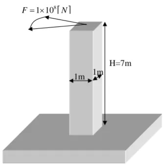
The approach described above has been applied to problems similar to one observed in engi-neering and nature. The configuration of a structure to be synthesized is one that is capable of supporting a highly variable load 7 meters above the ground. In addition, the structure is to be as lightweight as possible.
In order to provide a basis for comparison, a simple solution has been constructed to serve as a reference, illustrated in Figure 2.15. The solution is a straight vertical beam with a 1 meter by 1 meter cross section. The solution in Figure 2.15 corresponds to a fitness value of6.2054, by using equation 2.23, with the weightswand the degree of compensationsset according to Table 2.5.
Equation 2.23 provides an aggregate measure of performance between0and1, such that better performance corresponds to higher fitness such that the goal is to minimize the aggregated function. The inverse of equation 2.23 is used here, shown in equation 2.24 for fitnessFs.
Fs((µ1, ω1),(µ2, ω2), . . . ,(µn, ωn)) =
1
ω1µs
1+ω2µs2+...+ωnµsn
ω1+ω2+...+ωn
1
s
(2.24)
Nature has evolved phenotypes that address this problem in different ways. Trees, for instance, in addition to other functions, support loads generated by the their own structure and the wind. Bones support gravity and muscle loads.
H=7m [ ]
8
1 10
F= × N
1m 1m
[image:44.595.240.407.128.298.2]Figure 2.15: A simple reference solution.
Figure 2.17: The evolution of fitness values with respect to the number of generations. The vertical dashed lines show when the height of the load was increased.
As mentioned previously, the height of load morphogen is periodically increased during the evolutionary process.
2.14
Results
The simulated evolution was run in parallel on 70 processors for 24 hours. The initial population contained 400 individuals, each one starting with a random genome. Figure 2.17 shows the fitness value of the best phenotype in the population with respect to the number of generations, the dashed lines correspond to times during the evolution when the height of the load was increased. It can be seen that the fitness value oscillates during the evolutionary process. This phenomena corresponds to the increasing increments of the height of the load. After every increase, it takes several generations to evolve the phenotypes with respect to the new location of the load and thus to minimize fitness.
Figure 2.18 shows the fitness evaluation of the best phenotype once the load has reached the desired height of 7 meters. The dashed line corresponds to the fitness value of the reference solution. The evolved phenotype is approximately 3 times better in performance than the reference solution.
Figure 2.18: The evolution of fitness values once the phenotype has reached the desired height.
2.14.1 Phenotype Analysis
A typical developmental process of an evolved phenotype is shown in Figure 2.19. The devel-opment begins with a single cell and two morphogens (Figure 2.19a). The load is simulated by a vector force that randomly changes direction within the pink sector. Prior to the phenotype growing to reach the height of the load, it is only subjected to gravity (Figure 2.19b). Once the phenotype grows to reach the final height of the source of the load morphogen, the phenotype is subjected to the full load. The colors of the cells represent mechanical stress. Green corresponds to low stresses (below the yield stress), and red corresponds to high stresses (above the yield stress) (Figure 2.19c). The topology is similar to a pyramid, but unfortunately, almost all of the cells in the phenotype are over stressed (and are therefore colored red) indicating that this phenotype does not perform well in supporting the load (fitness = 102.54). As a result, this genome is unlikely to be selected for crossover, and therefore its genetic information is likely to be eliminated from the evolution.
a b c
Figure 2.19: Three stages during the developmental process of a single evolved phenotype. The colors represent mechanical stress. Green corresponds to low stresses (below the yield stress), and red corresponds to high stresses (above the yield stress). The white arrow represents the magnitude and principal direction of the load. The pink sector represents the range of variation of the direction of the load.
double helix (Figures 4.2a and b). This phenotype contains two primary modules (distinct structural elements) that are wrapped together and connected at multiple locations. The helix has a unique structural topology which makes it able to support loads that vary in direction.
Characteristics of modularity (i.e., distinct structural elements) can be observed in the evolved phenotypes. At this stage of the research the degree modularity of each phenotype cannot be quanti-fied, and therefore no measure is calculated or reported. However, both of the modular characteris-tics shown here have spontaneously emerged without directly imposing them in the fitness function or constraining the configuration of the phenotype.
2.14.2 Development Analysis
Figure 2.22 illustrates the embryogenesis of the helically shaped phenotype shown in Figure 4.2. Beginning with a single cell attached to the ground, the evolved set of rules guide the growth and development of the phenotype, as described below.
Figure 2.22e. Figure 2.22a. Initially, cell division occurs along the axis of the original cell facing towards the load morphogen, creating a vertical stack of 3 cells. Then the top cell in the stack divides laterally.
a b
Figure 2.20: Two views of a first phenotype (fitness value = 2.11), which is able to support the load, as indicated by the predominantly green color of the cells.
a b
Figure 2.22c. Growth of both elements continues. The 3rdcell from the top of the right-hand element divides laterally, creating the starting point for the 3rdmodular element.
Figure 2.22d. Growth of all three modular elements continues, approaching the load mor-phogen. Note that all cells are colored green, indicating that they are lightly stressed. A fourth modular element begins to grow diagonally into the ground near the left-hand side of the base of the structure.
Figure 2.22e. Growth of the composite structure continues and reaches the load morphogen, inducing load onto the structure, as reflected in the red color of many of the cells. The bright red color indicates cells that are carrying stress above the yield stress of the material. The second and third modular elements have merged (through the action of cell adhesion). The fourth modular element continues to grow diagonally upwardly and can be seen as the green cells extending to the right of the structure, near its base.
Figure 2.22f.Additional growth and adhesion of cells near the top of the two principal modular elements, results in reduction of the stress in all of the cells to levels below the yield stress of the material.
Figure 2.23 shows four different phenotypes which have been developed from the same geno-type. The first three have similar fitness values and similar topology with some degree of variation. The fourth phenotype has different topology, since it has not completely developed. Most of the cells are over stressed, which results in a higher fitness evaluation (and therefore lower performance).
Figure 2.24 shows the fitness evaluations of hundreds of phenotypes which were developed from the same genotype. Two peaks of the fitness values can be observed, with nearby distributions similar to a Gaussian distribution. Phenotypes with fitness values near the lower peak have topology similar to the phenotypes in Figures 2.23a, b, and c. The second group corresponds to phenotypes that perform more poorly (and hence have a higher fitness value) and are similar to the phenotype shown in Figure 2.23d. Due to variability in the environment, some phenotypes cannot complete their development process properly at some time step. The phenotypes which are able to continue developing after this time step usually continue to develop into successful mature phenotypes similar to those shown in Figure 2.23a, b, and c.
2.14.3 Genome Analysis
a b
c d
[image:50.595.134.515.110.654.2]e f
a b
c d
Figure 2.23: Four different phenotypes, growing from the same genome. The topologies of pheno-types a, b, and c, are almost identical, aside from small variations which result from the environment. The phenotype d has a visibly distinct topology.
0 1 2 3 4 5 6 7 8 9 10
0 10 20 30 40 50 60 70 80 90 100
Log (Fitness Evaluation)
[image:51.595.115.529.75.419.2]Number of Individuals
R1Z0S3hC7aV95gB9b6c6hC5gC0cB1h9b6cB2c4b0gDidiS5cDi R1113Z2W158tV72gB3b2c3bDiiiK
R1Z2W110bK
R1Z2A1dC0gB1g2c8gV72gB3b2c3bDiii R1Z0C5hV95gDifS2cC2hK
R2Z1W5tV102aS5a R1Z1W135gKC9g
Figure 2.25: The genome for the phenotype shown in figures 4.2 and 2.22 contains 9 different words.
contains four major characteristics: veto rules, anisotropic growth, cell division and cell death. The veto rules suppress the execution of this word when the phenotype reaches a certain age, which means that this word is executed frequently at the beginning of the developmental stage and pro-duces a large number of cells. The cell death rule separates a group of cells and promotes the creation of two struts in the phenotype. The shearing operation turns the struts into two helices which wrap around each other.
The mechanism of rapid cell production at the initial stage of development has also been ob-served in nature. Embryo cells divide much more frequently at the beginning of development than at maturity. The repetition of rules in the genome may be one of the factors that produces a degree of modularity in the phenotype [1].
2.14.4 Additional Runs
2.14.5 Constraints
As in practical engineering, where constraints play a major role during the design process, sev-eral physical constraints are active here, including thermodynamics and cell intersections,etc. An internal constraint to not grow ill-conditioned mesh configurations is imposed through the disease mechanism, which repairs or eliminates solutions with high numerical error. Additional constraints could be incorporated in the fitness function, for example phenotypes that exceed predetermined geometric limits can be given low fitness values. The advantage of not including such external constraints is that the evolutionary process is able to freely explore the design space, and synthe-size solutions that provide high levels of performance without being constrained to a predetermined configuration.
2.14.6 Robustness
Figure 2.26: Maximum mechanical stress, normalized to the material yield stress (σ/σy) vs. angle of the load vector.
Chapter 3
Asynchronous Scheme
The genetic algorithm in general uses a synchronize selection where the selection process is performed only after all the individuals are been evaluated prior to the mating scheme. In the direct encoding approach no development process is done and thus the variation in terms of evaluation between individuals is relatively small. In our model, the development process of every individ-ual is highly computationally intensive. In addition, there is a high variation in the development-computational time between different individuals within the population. Using a synchronization scheme in our model resulted in a low computational efficiency since the individual with the slow-est development process set the time of a single generation. Instead we have chosen to use an asynchronous evolutionary scheme which turns out to be much more computationally efficient and also increases the variability of the individuals during evolution, which eventually results in higher convergence rate. Unlike the synchronize scheme we do not wait until the last individual has been developed and evaluated. Instead, our only concern is to keep the nodes at a maximum capacity all the time. The number of nodes has to be smaller than the population size. For each time increment, an individual is been developed and evaluate on a single node, its fitness value is sent back to the master node. The master node will then send a new genotype for evaluation to the slave node. This process stops when there are no more genotypes to evaluate in the population. At this point the total number of individuals is given by,P opulationSize−N umberof N odes, whereP opulationSize
Chapter 4
Inhomogeneous Structures under Wind
Load
Inhomogeneous structures can be useful in many areas including optics, mechanics and thermal management, etc. In optics, for instance, several layers of thin films create an optical filter. Each layer has different properties which make the design of such filters highly complex. Different meth-ods have been developed for the synthesis of such filters. J. Skaar [7] has shown a way to synthesize optical thin-film filters with inhomogeneous properties such that each layer in the film has a differ-ent number of reflectors. Yang and Kao [8] introduced a way to evolve the structure of a thin film with inhomogeneous optical coatings such that the evolved structure has the functionality of a beam splitter and a narrow-band reflector.
In addition to the large variety of applications, new techniques have been introduced with the ability to fabricate highly inhomogeneous structures. These methods include molding and molding techniques [9] which enable inhomogeneity to be produced at the scale of a single micro-drop.
Our model provide the evolutionary process a tool to create inhomogeneous phenotypes, using the cell differentiation mechanism. In the following example, cells can be either made from steel or from aluminum.
4.1
Wind Load
which describes the behavior of a structure subjected to a wind as shown in equation 4.1. The parameterFi represents the load on nodei,F0is the total maximum load on the entire structure,S
is the structure’s volume andN is the number of cells. Equation 4.1 shows that an increase in the total volume will results in an increase of the total load in an exponential manner, this behavior is roughly describes a structure which is subjected to a wind. All the other parameters such as, gravity evolutionary scheme remains the same.
Fi =
F0
1− 1 S1/3
N (4.1)
4.2
Results, Inhomogeneous Structures under Wind Load
Figure 4.1 and Figure 4.2 show four different views of two phenotypes that have been evolved for several hundreds of generations. The colors of the cells in Figure 4.1a and 4.2a represent the dis-tribution of mechanical stresses inside the cells. Green represents low stress, graduates to red which represents high stresses. We can see that none of the phenotypes are over stressed. figures 4.1b andfigure 4.2b show the cell’s materials distribution in the phenotypes. We can see that both phe-notypes are inhomogeneous such that there exists regions of adjacent aluminum cells and regions of adjacent steel cells. A distinction between these regions are presents in figure 4.1c,figure 4.1d and figures 4.2c, and figures 4.2d.
The difference between both phenotypes in terms of performances is small. Both phenotypes have lower stresses and are relatively light. They also grew to the desired height. From a topological view, both phenotypes are completely different. The phenotype in figure 4.1 looks similar to a bar. The bar contain cross-sections with areas that ranged from high to low, from bottom to the top, respectively. We can also see that the inner part of the bar is made from aluminum Figure 4.1c, while the outer part made from steel Figure 4.1c. The second phenotype in Figure 4.2 has a topology which is similar to a two piece arc. The arc has two regions, upper and lower. The upper region is made from aluminum Figure 4.2c and the lower region is made from steel Figure 4.2d.
a b
[image:60.595.106.544.189.554.2]c d
a b
[image:61.595.109.542.192.546.2]c d
t = 0 t = 15
t = 30 t = 40
t = 50 t = 62
Chapter 5
Robustness
We present two different types of robustness mechanisms which have been spontaneously evolved
in silicoin a model of artificial embryogenesis. The first type provides robustness at the phenotype level, which is the ability of the phenotype to function in the presence of uncontrolled variations in the environment. The second type provides robustness of the growth process itself, which is the ability to grow a successful phenotype from a genome subject to environmental changes.
In our model, phenotypes grow in a stochastically changing environment from a simple set of rules (encoded in its genome) which are triggered by the environment, and have been evolved with evolutionary selection determined only by the fitness of the phenotypes to function in this environ-ment. We show that our evolutionary process is cable of evolving genomes which are robust in both ways. These types of robustness are critical for evolutionary synthesis of novel phenotype config-urations for two reasons. The environment, which serves as the trigger mechanism for regulation of the growth rules, changes significantly during the growth process. Additionally, the order of execution of the growth rules in a genome is random in our model.
a b c
Figure 5.1: Three different phenotypes from three different stochastic environment experiments (SEE).
5.1
Results
The asynchronous evolutionary scheme was run with an initial population of 400 individuals which corresponds to 400 different randomly generated genotypes. All genetic operations (se-lection, crossover, and mutation) have been performed at the genotype level at the end of every generation or “mating season”.
In the first three experiments the environment had high variability. We call this kind of exper-iment a “Stochastic Environment Experexper-iment” (SEE). We define the second kind of experexper-iments as “Fixed Environment Experiment” (FEE). In this experiment the environment (the external load) is held fixed. In all the SEE experiments, the same highly variable environmental effects were ap-plied, and the same evaluation scheme was used. In all experiments, the initial location of the load morphogen was 6 meters above the ground and the load was translated and scaled to the phenotype during grow