Beyond the KdV: Post-explosion development
L.Ostrovsky,1,2,a)E.Pelinovsky,2,3V.Shrira,4and Y.Stepanyants3,5,b) 1
NOAA Earth System Research Laboratory, Boulder, Colorado 80305, USA
2
Institute of Applied Physics, Nizhny Novgorod 603950, Russia
3
Department of Applied Mathematics, Nizhny Novgorod State Technical University, Nizhny Novgorod 603950, Russia
4
Department of Mathematics, Keele University, Keele ST5 5BG, United Kingdom
5
School of Agricultural, Computational, and Environmental Sciences, University of Southern Queensland, West St., Toowoomba, Queensland 4350, Australia
(Received 6 January 2015; accepted 24 March 2015; published online 5 August 2015)
Several threads of the last 25 years’ developments in nonlinear wave theory that stem from the classical Korteweg–de Vries (KdV) equation are surveyed. The focus is on various generalizations of the KdV equation which include higher-order nonlinearity, large-scale dispersion, and a non-local integral dispersion. We also discuss how relatively simple models can capture strongly nonlinear dynamics and how various modifications of the KdV equation lead to qualitatively new, non-trivial solutions and regimes of evolution observable in the laboratory and in nature. As the main physical example, we choose internal gravity waves in the ocean for which all these models are applicable and have genuine importance. We also briefly outline the authors’ view of the future development of the chosen lines of nonlinear wave theory.VC 2015 AIP Publishing LLC.
[http://dx.doi.org/10.1063/1.4927448]
In the aftermath of the revolutionary development in the theory of nonlinear waves in the 1960s–1970s, the inten-sity of studies in this field does not show signs of decreas-ing. Here, several lines of studies related to the KdV equation are surveyed. Focusing on generalizations of the KdV equation, we trace the development of main ideas and concepts of nonlinear wave theory yielding qualita-tively new solutions such as “fat” and table-top solitons, breathers, and slowly radiating solitons. The reasons underpinning the unmatched universality of the KdV equation as a mathematical model applicable in many physical contexts are quite natural: for long waves the model combines the most typical, small quadratic nonli-nearity and weak, small-scale dispersion. The balance between the nonlinearity and dispersion allows the possi-bility of solitary waves possessing astonishing particle-like properties such as robustness and persistence in colli-sions not only with each other but also with other pertur-bations. This particle-like behavior is at the origin of the term soliton introduced to emphasize the affinity of such waves with elementary particles (electrons, protons, etc). As the understanding of nonlinear waves matured, the limitations of the KdV model and necessity to go beyond it became apparent; hence, the trend towards developing more general and rich models which generalize the KdV equation and yield many new and non-trivial results. Here, we briefly discuss their appearance in various mathematical and physical contexts and some of the results which follow, such as qualitatively new types of solitons, their limiting shapes and parameters, and inter-actions. It is also demonstrated that these features are not
mathematical artefacts, which is illustrated by examples mainly related to nonlinear internal gravity waves in the ocean.
I. INTRODUCTION: MODEL EVOLUTION EQUATIONS
The basic equations describing evolution of long nonlin-ear dispersive waves were first derived in the end of the 19th century by Boussinesq (1872) and Korteweg and de Vries (1895). They were nearly forgotten until the 1960s, when the interest in these equations exploded. They proved central in the revolution in the understanding of nonlinear waves. The revolution was unfolding in several different, albeit related, directions. First, the “wave theory” supported by experi-ments began to establish itself as an important branch of mathematics and physics in the sense that various physical (as well as chemical, biological, and other) phenomena can be described by similar mathematical models, depending on such general characteristics as dispersion and nonlinearity. This, in turn, has resulted in identifying the key universal “model” equations, such as the KdV equation and many others. It has been realized that these asymptotically derived model evolution equations are universal and represent a powerful tool for studying nature. The surge in interest coin-cided and was partly caused by the discovery of remarkable mathematical properties of the key evolution equations: many of these nonlinear partial differential equations were found to be exactly solvable, and a new branch of mathemat-ical physics, often referred to as integrable systems, was born. These radically new mathematical techniques comple-mented by numerical simulations and novel asymptotic approaches have revealed the key role of solitary waves in the wave field evolution. Solitary waves first observed in a)Author to whom correspondence should be addressed. Electronic mail:
b)
All authors contributed equally to this work.
nature by Scott Russell in 1834 proved to be far from the structurally unstable homoclinic solutions such as separatri-ces in the ODE theory; on the contrary, they proved to be ro-bust solutions representing asymptotic behavior of a wide class of initial conditions. Moreover, the solitary solutions exhibited particle-like properties: in integrable equations sol-itary waves collide elastically, which gave rise to the term “soliton.”
At the same time, new asymptotic methods of solution of nonlinear evolution equations were developed, allowing to examine many physically important cases which cannot be reduced to integrable equations.
The revolutionary phase of the sixties and seventies of the last century was followed by a period of very extensive development characterized by an explosive growth of publi-cations in which the primary ideas were further developed and numerous new model equations, mostly integrable ones, were suggested and analyzed (many of them were written just as examples of integrability, without any asymptotic der-ivation from physically meaningful equations). Then, start-ing shortly before 1990, a deeper and more systematic development of the nonlinear wave theory began; both inte-grable and non-inteinte-grable equations found broader physical applications and, due to the progress in numerical modeling, were verified versus primitive physical equations.
The present paper aims to outline some of the latter developments related to the KdV-like systems, mainly those of the last 25 years. Note that nonlinear Schr€odinger equation could have been the subject of an equally interesting story, but here we concentrate entirely on the KdV and its “close rel-atives.” Here, we follow several key lines. One is studying broader classes of equations that describe wave fields with dif-ferent dispersion and nonlinearity as compared to the KdV equation. Second, we trace the enormous extension of the family of fundamental localized solutions which are often qualitatively different from those of KdV. Third, we discuss new applications. We mostly use as examples those taken from the context of internal gravity waves in the ocean; all main types of equations discussed below have established applications in the internal wave context. Moreover, for now the most numerous and diverse observations of solitons in na-ture apply to the oceanic internal waves.
Thus, what happened beyond the studies of the KdV equation? The universality of the latter is due to the simple physical approximation of generic weak (quadratic) nonli-nearity and generic weak dispersion represented by the third-order derivative
@u
@t þc
@u
@xþe au
@u
@xþb
@3u
@x3
¼0; (1)
wherecis the speed of long linear waves,aandbare con-stant coefficients, ande1 is a small parameter, character-izing smallness of nonlinear and dispersive terms. By making the Galilean transformation x0¼xct and t0¼et, this equation can be reduced to the canonical form
@u
@tþau
@u
@xþb
@3u
@x3 ¼0; (2)
where primes are omitted and all terms are of the same order. The balance between the nonlinear and dispersive terms in this equation leads, in particular, to stationary soli-tary waves—the solitons (we use here the term “stationary” for a translational wave of a permanent form, uðxVtÞ; in the coordinate system moving with the wave speedVsuch wave is indeed stationary as it depends only on spatial coor-dinate). The remarkable mathematical properties of this equation have been exhaustively studied (e.g., Refs.1–4).
To capture different wave dynamics, the first natural step is a straightforward extension of the nonlinearity and dispersion by retaining the next-order terms in the asymp-totic expansion. A rather general form of this extension, which has been derived by many authors to describe nonlin-ear waves in different physical contexts (see, e.g., Ref.5for surface and internal waves) is
@u
@tþau
@u
@xþb
@3u
@x3
þe a1u2 @u
@xþc1u
@3u @x3þc2
@u
@x
@2u @x2þb1
@5u @x5
¼0:
(3)
This equation combines quadratic and cubic nonlinear terms, linear dispersion of the 3rd and 5th order, and also nonlinear dispersion with the coefficients c1 and c2. In general, the
equation is not exactly integrable. However, Fokas and Liu6 found an asymptotic transformation of solutions of the extended KdV equation(3)for functionuto solutions of the KdV equation for a new auxiliary functionv
u¼vþe k1v2þk2vxxþk3vx
ðx
x0
vdxþk4xðavvxþbvxxxÞ
2 6 4
3 7 5;
(4)
where the coefficientskiare rational functions of coefficients
of Eq.(3). Thus, approximate solutionsu(x,t) to Eq.(3)can be obtained from the appropriate solutionsv(x,t) of the KdV equation(2)that are valid up toO(e2). Inasmuch as the KdV equation is completely integrable, one can say, that Eq.(3)is asymptotically integrable, i.e., it tends to an integrable one when e ! 0. This approach, although interesting, was not exploited thus far; the termsO(e) in Eq.(4)actually give just small corrections to the KdV solutions.
KdV solitons have a single free parameter apart from the “phase” specifying its position. The examples considered below are much richer in this respect.
For example, keeping the fifth-order derivative term results in the non-integrable equation known as the Kawahara equation7
@u
@t þau
@u
@xþb
@3u @x3þb1
@5u
@x5 ¼0: (5)
It possesses solitary waves with oscillating and decaying asymptotics which can form fairly complicated multisolitonic structures. Moreover, the Kawahara equation demonstrates important extensions of the very notion of a solitary wave. It possesses a class of coupled solitons also with more degrees of freedom than the classical KdV-type solitons.8 It also admits a class of “non-local” steady solitary waves consisting of a central “core” which resembles a classical soliton, and oscillatory, non-damping small amplitude “wings” which extend to both infinities. Such solutions were christened “nanopterons,”9which means “dwarf-wing”; the name is not often used, however. These objects can be viewed as solitary waves simultaneously radiating and absorbing a linear wave of small amplitude. These and other “quasi-solitons” which cannot be exactly localized or slowly attenuate due to radia-tion form a broad class beyond the scope of KdV; even in the case of slow damping they can form a useful intermediate asymptotics in the process.10Various aspects of their descrip-tion are often a mathematical challenge; they attracted a lot of attention in the literature (see, e.g., Ref.11). Some aspects of radiating solitary waves are discussed below in Sec.III.
Another generalization of KdV is adding a comparable cubic term to obtain the so-called Gardner equation which also exhibits important new classes of solitary waves, table-top solitons, and breathers. It will be considered in more detail in Sec.II.
The form of Eq.(3), even without a small parameter, is not universal. A more general form of a one-dimensional weakly nonlinear and weakly dispersive evolution equation resulting from asymptotic derivation can be written as
@u
@t þC uð Þ
@u
@xþG
@u
@x ¼0; (6)
where C(u) is the quadratic polynomial and G is a differential-integral operator obtained by the inverse Fourier transform of the linear dispersion relationc(k)1
G¼ ð 1
1
K xð zÞ@u @zðz;tÞdz;
K xð Þ ¼ 1
2p ð 1
1
c kð Þ c0
½ eikxdk; (7)
andc0 c(0) is the linear long-wave velocity. Evidently,
the KdV equation, as well as other evolution equations men-tioned above, are just particular cases of Eq.(6). For exam-ple, for the KdV equation C(u)¼au and G¼b@2/@x2. A more complicated example of an integral-differential
equation for which the very existence of a solitary wave is a non-trivial problem, is considered in Sec.III.
Finally, generalizations are also possible for some strongly nonlinear cases, although the applicability of “one-wave” evo-lution equations cannot be taken for granted. In these cases, the nonlinearity and dispersion cannot be completely sepa-rated, and the term responsible for the long-wave dispersion remains nonlinear. In Sec.IVwe show how much insight can be obtained using the understanding provided by weakly non-linear models even for strongly nonnon-linear dynamics.
The paper is organized as follows. In Sec.II, we discuss solitary solutions and long wave evolution in the Gardner equation. Sec. IIIdeals with the models containing two dis-persions, the short-scale (KdV-type) and long-scale (integral) dispersion, and discusses some peculiar properties of their solutions. Sec.IVdescribes strongly nonlinear model equa-tions, their limitations and applications. Finally, Section V summarizes the present state of understanding and gives some thoughts regarding the future of development in non-linear wave theory and applications.
II. GARDNER EQUATION: SOLITONS, KINKS, BREATHERS
A. Solitons
The Gardner equation
@u
@tþau
@u
@xþa1u 2@u
@xþb
@3u
@x3 ¼0 (8)
appeared in mathematical physics at the end of 1960s as an important example of completely integrable equations (e.g., Refs.2and3). Later, Lee and Beardsley5used this equation as the model describing strongly nonlinear internal waves observed in the ocean. Solitary solutions to the Gardner equation can be very different and depend on the sign of the cubic coefficient a1. Nonetheless, they can be presented as
the one-parameter family12
u xð ;tÞ ¼ A
1þBcoshðxVtÞ=D;
A¼ 6b aD2; B
2¼1þ6a1b a2D2; V¼
b
D2; U0¼ A 1þB;
(9)
whereVis the soliton speed,Dis its characteristic width, and U0 is the amplitude. The parameter B is in the limits
0<B<1 for a1<0 and B2>1 for a1>0. Soliton shapes
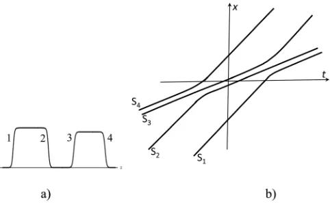
are shown in Fig.1fora>0 andb>0. At fixed signs of coef-ficients a and b, the soliton characteristics are qualitatively different for different signs of the cubic nonlinear term.
The first important qualitative departure from the KdV solitons is that whena1<0, the shape of solitons changes
sig-nificantly with increase of amplitudeU0from zero to the
lim-iting valueUlim¼ a/a1; namely, it goes from the bell-shaped
KdV soliton (B ! 1), to the table-top pattern (B ! 0, D2! 6a1b=a) with the infinitely increasing width (see Fig.
is always positive. The edges of this soliton are close to step-like transitions (kinks, or non-dissipative shock waves)13
u¼6 a
2a1
17tanhxVt 2D
; V¼ a
2
6a1 ;
D¼
ffiffiffiffiffiffiffiffiffiffiffiffiffiffi 6a1b a2 r
; (10)
where the signs correspond to the frontal (descending in space) kink and the rear (ascending) “anti-kink.” Note that these pat-terns are different from the kinks and anti-kinks in the sine-Gordon equation2,3where they are the only solitary solutions, whereas here they exist as the limit for a family of solitons.
In the case ofa1>0 (see Fig.1(b)), there exist two
dif-ferent families of solitons: “positive” solitons which, with increase in amplitude, vary from the KdV soliton to the soli-ton of the modified KdV (mKdV) equation2,3(Eq. (8) with a¼0), with no limitation on its amplitude; and “negative” solitons with the amplitudeU0<Umin¼ 2a/a1. In the case
ofU0¼Umin, the Gardner soliton(9)reduces to its limiting
form having algebraically (rather than exponentially) decay-ing asymptotics (u1/x2, when x! 1). This “algebraic” soliton has zero speedVin(8)(i.e., in the coordinate frame propagating with the linear long-wave velocity.) With the increase of amplitude jU0j Gardner solitons transform into
the mKdV solitons. In the range 0>U0>Umin, there are no
stationary solitons at all, instead there are more complicated nonstationary wave patterns calledbreathers2,3,73which are discussed below in more detail.
B. Interaction of solitons and kinks. Formation of soliton trains
Two-soliton interaction processes in Gardner equation are also quite peculiar.14 The interaction of solitons of the same polarity is similar to that in the KdV equation. This result can be interpreted within the framework of the approx-imate theory of interaction of solitons as particles with repulsing potential.15 If solitons have different polarities in the case of positive a1, the result is more interesting, since
the solitons can attract each other and form breathers, i.e., localized waves pulsating in the course of propagation. In this case, the breather solution can be found analytically.16 Depending on their parameters, they can take the form of ei-ther bound states of solitary waves of opposite polarity peri-odically interacting with each other (see Fig.2(a)), or in the form of envelope solitons whose carrier wave moves with a different velocity than the envelope wave, as in the nonlinear Schr€odinger (NLS) equation (see Fig. 2(b)). We emphasize that breathers exist only in the case of a positivea1and has
no analogues in the KdV equation.
[image:4.612.139.476.58.184.2]As mentioned, a non-trivial feature of the Gardner soli-ton close to the flat-top one is that it can be considered as a compound of kink and anti-kink (see above). The kinks behave quasi-independently in the process of interaction of two such solitons. In Ref.17, this problem was studied using asymptotic theory. As a result, the “double Toda” equation was derived for interacting kinks (the parameters a¼ a1¼6 andb¼1 were used):
FIG. 1. Soliton shapes in the Gardner equation(5)witha¼b¼1 for different soliton amplitudes. (a)a1¼ 1: line 1—KdV-like soliton, 2—“fat” soliton, 3—
table-top soliton with kink and anti-kink edges. (b)a1¼1: lines in the upper half-plane—“positive” solitons, line 4—one of the family of “negative solitons,”
[image:4.612.59.504.644.762.2]line 5—the limiting case of “negative” solitons: the algebraic soliton. Reprinted with permission from Grimshawet al., Physica D132, 40 (1999). Copyright 1999 Elsevier.
d2S
n dt2 ¼4 e
SnSnþ2eSn2Sn
ð Þ; (11)
whereSnare coordinates of kinks and anti-kinks; even
num-bersn correspond to frontal kinks, odd numbers n—to rear anti-kinks. If a kink–anti-kink pair belongs to the same Gardner soliton, then they are linked by the Katz–van Moerbeke equation realizing the degenerated B€acklund trans-form for the Toda equation.2,3,73 The main new element of this process as compared to interaction of solitons considered as a whole object is that, along with their behavior as par-ticles, they reveal the wavelike features. Figure 3illustrates this by showing trajectories of soliton fronts and rears in two interacting solitons having almost limiting amplitudes: the front of the rear soliton (numbered by 2) first affects the front of the first soliton (numbered by 4) rather than the much closer rear anti-kink(3)of the latter, and vice versa; this testi-fies to the remote action between the kinks.
When Eq.(11)is applied to chains of kinks, slow modu-lation of the chain can again be described by the Toda sys-tem, and the modulating envelope propagates with the “group” velocity three times greater than the “phase veloc-ity” of the carrier.
As can be expected from the integrability of the Gardner equation, its multisoliton solutions can be found by the inverse scattering method.14,18For negativea1and small
ini-tial amplitudes (<0.5Umin), the process of the solitons’
for-mation from a long initial pulse is similar to that in the KdV equation. For larger initial amplitudes, a leading table-top sol-iton is formed followed by smaller KdV-type solsol-itons and dis-persive tails.
C. Internal waves in the ocean: Solibores
Along with the KdV equation, the Gardner equation is being actively applied to various physical problems, in par-ticular, to studies of oceanic internal waves.27,65The coeffi-cients of the KdV and Gardner equations are determined by the integrals over depth of products of eigenfunctions of the linear boundary value problem. These eigenfunctions, in turn, depend on the vertical profiles of water density q(z) through the Brunt–V€ais€al€a (buoyancy) frequency
N zð Þ ¼
ffiffiffiffiffiffiffiffiffiffiffiffiffiffi g
q dq dz s
(12)
and shear flowU(z).
In coastal oceanic areas, nonlinear internal waves are typically generated by tides and often have a form of oscil-lating fronts (undular bores orsolibores) close to a sequence of solitons. Disintegration of a long initial perturbation into the Gardner solitons can be described using quasi-periodic solutions of the Gardner equation which have been found for both signs ofa1. As in the case of the KdV equation, these
solutions are expressed in terms of Jacobi elliptic functions. The periodic, slowly varying solutions are used to analyze the evolution of an initial front within the framework of the “dam break” problem, as disintegration of an initial stepwise perturbation. This approach was earlier suggested by Gurevich and Pitaevsky22for the KdV equation based on the Whitham equations1for a cnoidal wave with slowly varying parameters. It was then effectively applied to many physical problems, including the Gardner equation.23 If a1<0, a
weak initial step develops similarly to that in the KdV equa-tion; for a larger step, the leading wave is the table-top soli-ton. If a1>0, the evolution of a front is qualitatively
different. Both these cases are studied by Kamchatnov et al.23The Gardner-like solibores were observed, in particu-lar, by Henyey and Hoering.24
Unlike solitons, it is not easy to observe breathers in the ocean; still there exists some indirect indications of their occurence in the ocean.25Meanwhile, direct numerical simu-lations within the fully nonlinear Euler equations for three-layer water flow suggest the existence of long-lived internal wave breathers.26
In the context of internal waves in the ocean, the disper-sion coefficient bis always positive, whereas the nonlinear-ity coefficients aanda1can be of either sign. The mapping
of all coefficients of the Gardner equation was undertaken in Ref. 27 for the World Ocean based on the available hydro-logical data.
III. DOUBLE-DISPERSION MODELS. ROTATIONAL KdV: CAN IT SUPPORT SOLITONS?
A. Rotation modified KdV equation
Now we consider another extension of the KdV model which makes the equation non-integrable. As mentioned, the KdV equation combines the effects of weak nonlinearity and weak, “small-scale” dispersion (the dispersion which mani-fests itself in the short wavelength range). In the linear limit, it corresponds to the dispersion relation in the form x¼ckbk3 where the last term is small. Another practi-cally interesting class of waves includes the “large-scale” dispersion in addition to the small-scale one. If it is also weak, then the dispersion relation takes the form x¼ckbk3þc/k.This kind of dispersion is characteristic of waveguides in electrodynamics, acoustics, optics, and, as will be discussed here, waves in rotating fluids.28The corre-sponding generalization of the KdV equation contains an in-tegral dispersive term
[image:5.612.54.295.57.206.2]@u
@tþc0
@u
@xþau
@u
@xþb
@3u @x3 ¼c
ðx
1
udx0: (13)
After differentiation with respect tox, this equation takes a more convenient form
@ @x
@u
@tþc0
@u
@xþau
@u
@xþb
@3u @x3
¼cu: (14)
As with the Gardner equation, this equation was obtained long before the 1990s for oceanic waves experienc-ing the influence of Earth rotation28 and then has attracted much attention of both mathematicians and physicists due to its unusual properties; later it was dubbed the “Ostrovsky equation” (see, e.g., Refs.29–31); here we call it the rKdV equation. Similar equations were derived in other contexts, in particular, for waves in random media32and for waves in rotating plasmas.33
Note first that in its general form Eq. (14) is non-integrable; moreover, even its stationary solutions have not been obtained in the analytical form thus far. However, some interesting rigorous results were formulated for this equation from the very beginning. It is easy to see that any finite per-turbation described by this equation has zero total “mass”: MÐuðx;tÞdx¼0, where the integration is taken either over the period of a periodic wave or over the entire axisx for localized perturbations. This zero-mass restriction, appa-rently, has no grounds in basic physics and appears only as a consequence of the approximations adopted in derivation of Eq.(14); there is no such constraint within the set of primi-tive equations. An interesting issue of how an arbitrary initial perturbation with the non-zero total mass adjusts to suit Eq. (14)has been considered by Grimshaw.29
Another important rigorous result is the “anti-soliton theorem” established in Ref. 34 and then reproduced in numerous other papers. The theorem states that whenb>0 (which is the oceanic case) there are no stationary solitary solutions to Eq.(14). However, the existence of such solu-tions is not prohibited ifb<0; the specific solitary solutions with zero total mass were constructed numerically in Ref. 33. It was shown that they can form stationary bound states in the form of multisolitons and even regular or random chains of solitons (cf. notes about the Kawahara equation(5) above). The phase space of the stationary version of Eq.(14) can be fairly complicated; some stationary solutions were studied in Refs.35 and 30. The detailed description of all possible stationary solutions is a challenge which, hopefully, will be resolved in forthcoming studies.
B. Reduced rKdV
More successful were analytical studies of the reduced case of Eq.(14)which is valid if the wave is long enough to neglect the short-wave (KdV-type) dispersion
@ @x
@u
@t þc0
@u
@xþau
@u
@x
¼cu: (15)
The stationary solutions of Eq.(15) depending on one variablef¼xV t,V¼const, satisfy a second order ODE and thus can be studied relatively easily. It was shown28 that there exists a class of smooth “fast” (V>0) periodic waves, limited in amplitude by a wave of parabolic shape; evidently, an unlimited parabola is also a solution of the full equation (14). The “slow” stationary waves are non-smooth and limited in space. Later, stationary solutions of Eq. (15) were classified in Ref. 36. Among them there are singular solitary waves with sharp crests dubbed peakons and cuspons. Even more complicated loop soliton solutions were constructed and their interaction was studied (see, e.g., Ref. 37 and references therein), but all such non-smooth solutions are structurally unstable; they disappear as soon as any of neglected physical factors such as dissipa-tion or small-scale dispersion are taken into account;36 on the contrary, solutions of the full equation are smooth as long as the initial condition is smooth.
Thus, a non-trivial problem concerning the reduced rKdV equation(15)is to find the condition under which the initial perturbation eventually becomes singular (breaks) or, on the contrary, remains smooth at all times in the process of wave propagation. It has been shown in Ref. 38 that if the initial condition u(x, 0)¼u0(x) is such thatd2u0(x)/dx2>c/
3aat somex, then wave breaking eventually occurs and the solution becomes singular. Ifd2u0(x)/dx2<c/3afor allx, the
solution remains smooth at all times. Note that earlier a pa-rameter39 Os¼3aK/c dubbed as the “Ostrovsky number” was introduced, where K is the maximum curvature in the initial condition; on the basis of this parameter, the authors estimated the possibility of wave breaking in Eq. (15). The physical basis for that is a “competition” between wave steepening due to nonlinearity (as in non-dispersive simple waves) and its deformation due to the long wave dispersion which, unlike the small-scale dispersion in the KdV equa-tion, is not always able to prevent wave breaking. Moreover, in the non-breaking case, Eq. (15) can be reduced to the completely integrable Tzitzeica equation (known also as the Dodd–Bullough–Mikhailov equation) (for details and further references see Ref.39).
C. Soliton evolution in rKdV
Rather non-trivial are non-stationary solutions of Eq. (14). According to the aforementioned “antisoliton theorem,” an initial KdV soliton cannot exist infinitely; it gradually decays due to radiation.42 As a result its amplitude A(t) attenuates adiabatically as (t0t)
2
where t0 /
ffiffiffiffiffiffiffiffiffiffiffiffiffiffiffiffiffi Aðt¼0Þ p
, and at tt0 the soliton is extinct, being completely
con-verted into a radiated wave (terminal damping). The situa-tion can, however, radically change if a KdV soliton interacts with a long wave close to the solution of Eq.(15). These two waves exchange energies, and the losses due to radiation from a soliton can be compensated by pumping from a long wave so that a solitary wave can exist in this environment. In the numerical example shown in Fig.4, the soliton amplitude periodically changes due to the energy exchange with a long wave.
In particular, a stationary wave can be formed in which a soliton is sitting on the long wave crest or trough. As fol-lows from the numerical modeling, the former configuration is stable and the latter is unstable. It is interesting that, as our preliminary studies show, ifonly onesoliton is traveling on a periodic wave, the result is the opposite: the soliton equilib-rium position on the crest is unstable, whereas its position at the trough is stable. This difference is due to the fact that in the latter case, soliton radiation is a pure loss, whereas in the fully periodic case the soliton radiation can be compensated by that from the solitons ahead of it.
The important outcome of these studies is that, notwith-standing the “anti-soliton theorem,” waves close to solitons can exist on a variable background such as a long periodic wave co-propagating with them. Chen and Boyd41 found some other non-trivial wave shapes; among them are solitary
waves of alternative polarity sitting on the crests of a back-ground long wave.
The list of non-trivial features of rKdV equation (14) can be continued. Recently, it was shown that in the long-term evolution, the initial KdV soliton in Eq. (14) with bc>0 ends up as a specific envelope soliton which looks similar to that in the NLS equation, but its carrier sinusoid frequency always corresponds to the inflection point of the dispersion curve x(k) where the group velocity has a local maximum.31 The same phenomenon was observed also in the context of waves in periodic lattice structures.44Figure5 demonstrates the evolution of the KdV soliton into the NLS envelope soliton. At the beginning, the KdV soliton experi-ences a terminal decay as described above, but after a long time it evolves into a stable NLS-like soliton whose phase and group speeds are different. If bc<0 in Eq. (14), then one can construct a stationary NLS-like soliton33 whose phase and group speeds are equalVp¼Vg¼2(bc)1/2;
more-over, the phase speed is maximal on such a soliton.
It is noteworthy that the effect of transformation of a KdV soliton into an NLS-like soliton was observed in the laboratory experiment in a rotating tank.45 Furthermore, a general analysis of the modulation stability of quasi-harmonic waves in the NLS equation following from Eq. (14) has shown that the modulational instability occurs for waves with wavenumbersk>kc, wherekc¼(c/3b)1/4. In the
[image:7.612.52.297.462.720.2]case of KdV equation (c¼0), quasi-harmonic waves are always stable with respect to modulational instability for any wavenumbers.2There is an apparent paradox in that the rota-tion effect (c6¼0) leads to modulation instability at large rather than at small wavenumbers. This phenomenon is explained by the suppression of a zero harmonic by rotation. It appears in higher orders and cannot contribute to the
FIG. 4. Adiabatic interaction of a strong KdV soliton with a periodic wave of quasi-parabolic profile satisfying Eq.(14).43From bottom to topt¼0 (a),
[image:7.612.324.548.488.718.2]t¼0.4 (b),t¼1 (c). Reprinted with permission from Gilmanet al., Dyn. Atmos. Oceans23, 403 (1996). Copyright 1996 Elsevier.
nonlinear coefficient of the NLS equation making the equa-tion modulaequa-tionally unstable fork>kc.
D. Generalizations of rKdV
Similar to the KdV case, Eq. (14)can be supplemented by cubic nonlinearity to obtain the rotation modified Gardner equation
@ @x
@u
@t þc0
@u
@xþau
@u
@xþa1u 2@u
@xþb
@3u @x3
¼cu: (16)
This equation, currently known as the Gardner–Ostrovsky equation, was suggested in Ref.50 for internal waves in a rotating ocean when the interface between two layers (the pycnocline) is located at the depth close to the half of the fluid depth. The terminal decay of solitons ata1<0 due to
large-scale dispersion was studied in Ref.46. It was revealed that solitons of relatively small amplitude (quasi-KdV soli-tons) decay in accordance with the prediction of adiabatic theory, whereas the decay of large amplitude solitons having a table-top shape can occur non-adiabatically from the very beginning. The direct numerical modeling of Eq.(16)shows that the shape of table-top solitons distorts at the very early stage of evolution. The influence of large-scale dispersion on decay of another kind of solitons (whena1>0) and breathers
has not been studied thus far.
The particular case of Eq. (16) with a ¼ 0 (rotation modified mKdV equation) has been studied more thor-oughly. This equation was derived and studied in a different physical context, in particular, for ultrashort optical impulses in nonlinear dielectrics (see, e.g., Ref. 47 and references therein). The large-scale dispersion in this case is caused by the polarization effect.
The reduced version of Eq. (16)witha¼b¼0 can be integrable, but the criterion for integrability is rather intri-cate. This problem was studied by Johnson and Grimshaw.48 They thoroughly studied the wave breaking conditions depending on the initial wave steepness and found a link of that equation to the sine-Gordon equation.
E. Oceanic applications
Equations (14) and (15) are often applied in physical oceanography where, as mentioned, soliton-like groups of internal gravity waves are common. In particular (e.g., Refs.49 and 50) it was shown that rotation decreases the number of solitons formed in a given tidal cycle. Later, Grimshawet al.51analyzed non-stationary processes for re-alistic oceanic parameters. Li and Farmer39 made specific calculations within the framework of these equations to-gether with the direct numerical simulations of the corre-sponding hydrodynamic equations to analyze the data of experiments in the South China Sea. In particular, they con-firmed the aforementioned result regarding suppressing sol-iton formation by rotation.
IV. STRONGLY NONLINEAR KdV-TYPE MODELS
A. Stationary waves: History
Can KdV and its modifications be extended to strongly nonlinear waves? A measure of nonlinearity can be, for example, the ratio of maximal fluid velocity in a wave to its propagation velocity in linear approximation; this ratio cor-responds to the Mach number in gas dynamics. Classical examples are non-dispersive waves in mechanics of com-pressible media where the important basic classes of solu-tions are the simple (Riemann) and shock waves. The theory of strongly nonlinear dispersive waves is not well developed, especially for multi-dimensional waves such as internal waves in the ocean. In many cases, the direct numerical sim-ulation (DNS) of the basic equations is used for each specific problem. Still, a noticeable progress in derivation and appli-cation of strongly nonlinear model equations can be reported. We consider this problem in the context of stratified fluid flows, including internal waves.
An additional difficulty in obtaining model equations as compared with the weakly nonlinear waves considered above is that the dependence on vertical coordinatezcannot be sep-arated from the horizontal ones and, consequently, there is no fixed modal structure. The early results were obtained for stationary 2D motions in which all variables depend onzand f¼xVt where V¼const. For these flows, the hydrody-namic equations can be reduced to one equation52 for the stream functionw
WffþWzzþV2N2ðzW=VÞW¼0; (17)
whereN(z) is the Brunt–V€ais€al€a frequency (see Eq.(12)). Equation(17)has been widely used in numerical model-ing. A remarkable feature of this equation is that it evidently becomes linear ifN(z)¼const. Therefore, stationary progres-sive waves (but only stationary!) are described by a linear equation and hence, can have, in particular, a sinusoidal pro-file of arbitrary amplitude. The majority of other analytical results were obtained for stationary waves in a two-layer fluid with a density jump between the homogeneous layers. The first study using this approach was, apparently, made in Ref.53. It was found that there exists maximal possible soli-tary wave amplitude at which it acquires a flat-top shape and tends to two infinitely separated kinks. Qualitatively this pat-tern is similar to the solutions of the Gardner equation dis-cussed above, but now it is valid for an arbitrarily strong wave. For a two-layer fluid limited by immovable horizontal surfaces from top and bottom, with upper layer thicknessh1
and lower h2and densitiesq1andq2>q1, the amplitude of
the interface displacementg(x,t) and propagation velocity of such a limiting soliton are
Amax¼
h1h2 ffiffiffia p
2
h1h2
2 ;
Vmax¼
ffiffiffiffiffiffiffiffiffiffiffiffiffiffiffiffiffiffiffiffiffiffiffiffiffiffiffiffiffiffiffiffiffiffiffi gð1aÞðh1þh2Þ p
1þpffiffiffia
ffiffiffiffiffiffiffiffiffiffiffiffiffiffiffiffiffiffiffiffiffiffi g0 h
1þh2
ð Þ
p
2 ; (18)
where a¼q1/q2,g0¼g(1a)a. The approximate equalities
close to unity; this so-called Boussinesq approximation is well-suited to oceanic conditions where density variations in water are always small. Moreover, in the same case, the free water surface can still be assumed immovable (rigid lid approximation) since surface waves do not significantly affect internal motions (not vice versa, though). In what fol-lows for simplicity we consider this case.
From Eq. (18) follows a significant result: the polar-ity of a soliton (the sign of Amax) is specified entirely by
the difference h1h2. As a consequence of that in the
oceanic solitons, the displacement is always directed towards the thicker layer. There are no solitary solutions whenh1¼h2; for smalljh1h2j nonlinearity is weak and
solitary solutions can be described by the Gardner equa-tion. Figure 6 illustrates shapes of solitary waves at dif-ferent amplitudes.54
B. Non-dispersive waves
Subsequently, effective numerical codes for directly solv-ing the fully nonlinear 2D problems were developed both for stationary and non-stationary solutions. Our goal, however, is to answer the same question as above: is it possible to reduce the 2D problem to one-dimensional equations (or the 3D problem to 2D equations) by separating thez-dependence? As mentioned, the strict answer is no: one cannot separate verti-cal dependence from horizontal. However, some effective long-wave equations have been obtained for strong nonlinear-ity, primarily for the two-layer model, where at least one exact result can be obtained. For very long waves, dispersion can be completely neglected (the quasi-hydrostatic approximation). In this case, as expected, the interface wave can propagate as a simple wave with the local velocity55
cð Þ ¼g 6c0 1þ3
h1h2
ð Þðh1h22gÞ h1þh2
ð Þ2
ffiffiffiffiffiffiffiffiffiffiffiffiffiffiffiffiffiffiffiffiffiffiffiffiffiffiffiffiffiffiffiffiffi h1g
ð Þðh2þgÞ h1h2 s
h1h22g h1h2 2
4
3 5 8
< :
9 =
;; (19)
wherec0 c(0) is the long linear wave velocity. The
de-pendence(19)on local displacementgis shown in Fig.7for three depth ratios corresponding to available observational data.
Here, the long wave velocity non-monotonically depends on the local displacement. Thus, unlike the classical dynamics of compressible fluid, the waves of “compression” and “rarefaction” can exist for any sign of displacement gra-dient. It is interesting thatcðgÞreturns to its linear value at g¼(h2h1)/2, which coincides with the maximal amplitude
of the soliton given in(18). As in the 1D dynamics of com-pressible fluids based on simple waves, the full description
of bi-directional non-dispersive internal waves can be devel-oped using Riemann invariants.
[image:9.612.332.540.528.717.2]Recently, a 2D generalization of the notion of a sim-ple wave for a continuously stratified fluid was found.57 These solutions have the form f(n,b), where bis the ver-tical coordinate of a fixed isoline of density (isopycnal line), and n¼xc(x)t is the implicit variable. In such waves all perturbations in a fixed vertical cross section propagate at the same velocity, but vertical structure of the field is different in each cross-section. This solution was validated by comparison with the direct numerical simulation.
FIG. 6. Displacement profiles in a soliton,g(x)/h1 vsx/h1 for two-layer fluid withh2/h1¼3,q2/q1¼0.997 (surface is atþ1, and bottom is at3
[image:9.612.67.284.531.685.2]on the vertical axis).54The lines depict the pycnocline depressions caused by a soliton from 0.05 to 0.99 at the center. The dashed line marks the level of limiting amplitude. Reprinted with permission from W. Evans and M. Ford, Phys. Fluids8, 2032 (1996). Copyright 1996 American Institute of Physics.
FIG. 7. Simple wave velocity versus local interface displacement for h1/
C. Model equations for dispersive waves
When the dispersion, albeit weak, is crucial (which is always true for solitary waves), it is natural to try to obtain model equations generalizing the weakly nonlinear models such as Boussinesq, KdV, and Benjamin–Ono equations. For these cases, a long-wave approximation can be constructed using the corresponding expansion of dispersive terms while keeping the nonlinearity strong. Actually, this basic approach was first suggested by Whitham58 for surface waves based on the expansion of the Lagrangian; the later work by Green and Naghdi59includes a sloping bottom. For internal waves in a two-layer case, Miyata60 suggested Boussinesq-type long-wave equations for strongly nonlinear, weakly dispersive waves in a two-layer fluid, and con-structed a stationary solitary solution of these equations. A comprehensive analysis of this problem for a two-layer fluid was performed by Choi and Camassa.61 Thus, we call the corresponding equations the MCC system. They have the form
gt¼ ½ðh2h1Þu2; ðu1u2Þtþu1u2xu2u1xþg0gx¼D; (20)
where
D¼ 1
3ðh1þgÞ
h1þg
ð Þ3 u1xtþu1u1xxu21x
n o
1
3ðh2gÞ
h2g
ð Þ3 u2xtþu2u2xxu22x
n o
: (20a)
The termDis responsible for the weak nonlinear dispersion (non-quasistatic approximation); it is obtained by expansion of the higher-order terms in hydrodynamic equations. Even earlier, Choi and Camassa62 obtained similar equations for the case of an infinitely deep lower layer, in the approxima-tion analogous to that used for the Benjamin–Ono equaapproxima-tion.
Within the framework of Eqs. (20), the description of stationary waves can be reduced to a second-order ODE. In particular, the velocityffiffiffiffiffiffiffiffiffiffiffiffiffiffiffiffiffiffiffiffiffiffiffiffiffiffiffiffiffiffiffiffiffiffiffiffiffiffiffiffiffiffiffiffiffiffiffiffiffiffiffiffiffiffiffiffiffiffiV of a soliton of amplitude A is
g0ðh
1AÞðh2þAÞ=ðh1þh2Þ p
:
Equations (20) were generalized to include a bilinear shear current profile.63 For stationary waves, an interesting development was suggested by Voronovich:64 stationary long-wave solitary solutions were found for a two-layer fluid in which each layer is exponentially stratified so that the buoyancy frequency N is constant in each layer (the “2.5-layer model”). According to Eq. (17), the solution in each layer is still linear which allows a relatively simple descrip-tion. Note that in this case the solution may include an inter-nal vortex core.
The above models, however, have a common inconsis-tency. They assume a weak dispersion (long-wave approxi-mation), whereas the nonlinearity can be arbitrarily strong. On the other hand, a soliton can exist in the case of essential balance between the nonlinearity and dispersion so that the corresponding approximations should be verified in each case. Fortunately, the direct numerical modeling shows that they work well in a rather broad range of wave parameters.56
The next step was to write a one-directional evolution equation generalizing the KdV and BO equations in which the nonlinear long-wave velocity for the two-layer model is taken in the exact form(19), whereas the dispersion parame-ter corresponds to a local instantaneous displacement at each point of the wave profile.56Thus, the strongly nonlinear ana-log of the KdV equation (the “b-model”) has the form
@g
@t þcð Þg
@g
@xþ
@ @x b gð Þ
@2g @x2
¼0; (21)
whereb¼cðgÞðh1gÞðh2þgÞ=6 is the dispersion
parame-ter which locally corresponds to the KdV dispersion at each point of the wave. A modification of the “b-model”(21), the so-called “E-model,” as well as a similar generalization of the Benjamin–Ono (BO) equation, were also suggested in Ref.56.
D. Oceanic observations
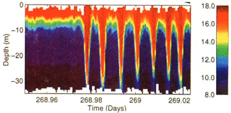
From the 1990s experimental observations of strongly nonlinear internal solitons became ubiquitous,65 although some single observations were reported even earlier. In cer-tain cases, weakly nonlinear models such as the KdV and Gardner equations describe them well. In general, however, strongly nonlinear models are necessary. A characteristic example is the Coastal Ocean Probing Experiment (COPE) off the coast of northern Oregon performed in 1995 (Fig.8), which shows a long sequence of tide-generated solitary impulses.66As seen from Fig.8, the depression of the sharp pycnocline (often approximated by a density jump in theory) reaches a depth 5–6 times its initial position (from 5 to 30 m in Fig.8). Although even stronger solitons were observed in the ocean, this ratio is, perhaps, the “world record of nonlinearity.”
[image:10.612.321.554.602.716.2]In Ref. 66, the Gardner equation was used beyond its formal range of applicability as a fit for the shape of an indi-vidual soliton. In Ref. 17, the kink interaction model (11) was applied to the same data to predict evolution of a group of strong solitons. A more consistent and detailed theoretical analysis of these and other data was performed in Ref. 56 using the MCC equations and the b- and E-models. Remarkably, the dependencies of soliton velocity on its am-plitude provided by these models are close to those obtained from the direct numerical simulation. For the soliton width,
these results are close for moderate ratiosq¼h2/h1; for the
case ofq>10–12, significant discrepancies occurred; how-ever, even in these cases the agreement with the DNS and experimental results is much better than with those using the KdV solitons.
Numerous other observations of strong internal solitons and their groups have been reported in different areas of the ocean.65,67
V. CONCLUSIONS AND PERSPECTIVES
From a close distance, a panorama of any scientific field might look chaotic, but a quarter of a century span allows us to choose and follow up upon a few coherent threads in the recent phase of our chosen corner of nonlinear wave theory. Here, we will briefly summarize the key points and ideas described above and try to make a guess about their possible development in the future.
It has been demonstrated how the account of higher-order nonlinearity and/or dispersion allows one to capture qualitatively new wave dynamics as compared to the classi-cal KdV model. The point to be emphasized first is that for a qualitative change to occur in a weakly nonlinear model, a mere degeneracy of coefficients of the quadratic nonlinearity and/or leading order dispersion is quite often sufficient to obtain these new dynamics. The Gardner equation provides an excellent example of such an extension: its solitary solu-tions vary from bell-shaped to “fat” and table-top solitons; kinks are also solutions; solitons of any polarity and breath-ers can co-exist when the cubic term coefficient is positive. Integrability of the Gardner equation made it possible to ana-lytically obtain the full picture of interactions between soli-tons of various types and between solisoli-tons and non-localized waves. Further development of asymptotic methods made it possible to describe multisoliton and multikink ensembles in both integrable and non-integrable systems, including the “hierarchy” of such ensembles allowing one to build a high-order ensemble as an envelope over the previous one.
Extensions of the KdV equation with higher-order dis-persion and integral disdis-persion considerably enrich the fam-ily of solitary waves and possible scenarios of wave dynamics. They provide examples of solitons with non-monotonic structures, coupled solitons, multisoliton fronts and groups, as well as stationary random sequences of coupled solitons. When steady solitary waves cannot exist on a constant background due to radiation losses, they can propagate long enough in the form of gradually decaying “radiating solitons” and serve as intermediate asymptotics, possibly evolving into wave packets—the envelope solitons mentioned in Sec.III. Solitons, which asymptotically decay in the absence of a background can, exist indefinitely if they exchange energy with a variable background. The richness of the evolution scenarios provided by the evolution equa-tions with integral dispersion seems to be limitless, but to advance in their understanding new methods of analysis have to be developed. We definitely expect this thread to continue well into the future.
The generalizations of KdV mentioned above still corre-spond to weakly nonlinear and weakly dispersive waves in
physical applications. The theory of “genuinely” strongly nonlinear waves in dispersive media is an extremely difficult and not very well developed part of the wave theory. Direct numerical simulations of the evolution of strongly nonlinear waves are necessarily computationally expensive and not always easy for interpretation, which makes it practically impossible to sweep a multidimensional parameter space. Remarkably, relatively straightforward modifications of weakly nonlinear equations including KdV have proved able to capture strongly nonlinear patterns in good agreement with the DNS and experiments.
We want to emphasize that all, sometimes bizarre, prop-erties of the soliton zoo described above are not exotic: such waves do exist in many real physical environments as exem-plified by internal waves in the oceans. It is essential that, in the latter case, the 1D (2D) evolution equations describe 2D (3D) waves with an appropriate depth distribution. For weak nonlinearity, these waves are multimodal, and the results are different for different vertical modes. For strongly nonlinear waves, which cannot be presented by a few fixed modes, manageable results have so far been either for non-dispersive (simple) waves or for a two-layer model of stratification. Nonetheless, in all cases considered above, not only a quali-tative but also a quantiquali-tative (albeit approximate) agreement with observation was obtained in a number of cases.
Let us now briefly speculate about what can be expected in short- and long-term perspectives in the corner of the non-linear wave theory visited in this paper, and beyond that.
A shortage of room forced us to leave aside many prom-ising threads related to our main topics. Among them is the development of a statistical description of ensembles of essentially non-sinusoidal waves whose deterministic evolu-tion we have discussed above. One of the developing direc-tions is “soliton turbulence” for integrable models where substantial progress has been made in kinetic description of soliton ensembles (“soliton gas”).19 In contrast to hydrody-namic turbulence where there are clear sources and sinks of energies providing universal turbulence spectra (such as in the Kolmogorov turbulence), in the integrable models the random soliton ensembles can produce various scenarios of very complex dynamics, but retain dependence on the initial distribution of their parameters. Studies of evolution of the wave field momenta during elementary interactions of soli-tons carried out within the KdV and mKdV equations20,21 will certainly be extended for other models, including non-integrable ones.
of a second wave which leads to modification of the instabil-ity domain. Coupled equations describing vector solitons in plasmas and chains of particles70yield a new type of solitary waves—helical solitons. Study of their properties, unusual features of interaction, the role in the energy transport in bio-molecules represents intriguing issues which are likely to attract attention in the nearest future.
We were unable to survey significant progress in studies of two-dimensional generalizations of the KdV equation, the Kadomtsev–Petviashvili, Zakharov–Kuznetsov, and other equations which possess multidimensional fully localized solitons, the lumps.2,3,73 Returning to the area of our main physical example, the oceanic internal waves, we only very superficially mentioned a rich body of field observations and totally passed over laboratory modeling of internal solitons. We expect all these threads we barely mentioned here and some others which were not mentioned to flourish and bring important new results yet in the next decade. We also antici-pate progress in derivation and numerical justification of strongly nonlinear evolutional models.
Much more difficult is to forecast, even roughly, the subsequent development in the upcoming decades. What shall a reader see in the Chaos issue dedicated to the 50th an-niversary of the journal in 2041? All we dare to predict is a series of “Grand Unifications” (borrowing the terminology from quantum field theory).
The firstof them is a much closer intertwining of analyt-ical models, computations, and physanalyt-ical experiments. We believe that, in spite of the increasing prominence of the lat-ter two, model equations will retain their key role as the first step in identifying and qualitative understanding of new phe-nomena, as well as selection of the most promising future directions of research. We will see increasing numerical efforts applied to both the model evolution equations and primitive equations.
Second is the overlapping of different effects and mod-els in nonlinear wave theory. We have already seen that the long-wave soliton can be transformed to an envelope soliton due to radiation in a rotational system. An opposite process can be represented by super-short (femtosecond) laser impulses which can have a length of only a few carrier wave periods47and their description as “envelope waves” becomes insufficient.
Thirdis the merging of various approaches originated in different areas of nonlinear wave theory. In particular, lack of space forced us to abandon touching a very important class of “autowaves” existing, in particular, in biological media such as nerve fibers and in some chemical reactions (e.g., Ref.72). They are typically considered separately from quasi-conservative waves like KdV solitons and even from oscillating waves in active media such as laser impulses. We will see development and adaptation of relevant asymptotic methods for description of such processes; in fact, such a de-velopment has already started.74
Fourth, the progress of experimental techniques with application of new methods and equipment can provide sur-prising discoveries in nonlinear waves (a good recent exam-ple is the development of the method of direct observation of
the dispersion relation of surface water waves in a laboratory45).
And it is most easy to predict that there will be many unpredictable events in both theory and experiment. We are looking forward to seeing these events and hope that young generation of scientists will bring them forward.
ACKNOWLEDGMENTS
E.P. and Y.S. were supported by the Russian State Project No. 5.30.2014/K; E.P. was also supported by Volkswagen Foundation and RFBR Grant No. 14-05-00092.
1
G. B. Whitham,Linear and Nonlinear Waves(Wiley, New York, 1974).
2M. J. Ablowitz and H. Segur, Solitons and the Inverse Scattering Transform(SIAM, Philadelphia, 1981).
3
R. K. Dodd, J. C. Eilbeck, J. D. Gibbon, and H. C. Morris,Solitons and Nonlinear Wave Equations (Academic Press, London, 1982); A. C. Newell, Solitons in Mathematics and Physics (SIAM, University of Arizona, 1985).
4
A. R. Osborne, Nonlinear Ocean Waves and the Inverse Scattering Transform(Academic Press, Boston, 2010).
5
Ch.-Y. Lee and R. C. Beardsley, J. Geophys. Res. 79, 453 (1974); R. Grimshaw, E. Pelinovsky, and O. Poloukhina, Nonlinear Processes Geophys.9, 221 (2002); A. Karczewska, P. Rozmej, and E. Infeld,Phys. Rev. E90, 012907 (2014).
6
A. S. Fokas and Q. M. Liu,Phys. Rev. Lett.77, 2347 (1996).
7
T. Kawahara,J. Phys. Soc. Jpn.33, 260 (1972).
8
K. A. Gorshkov, L. A. Ostrovsky, V. V. Papko, and A. S. Pikovsky,Phys. Lett. A 74, 177 (1979); K. A. Gorshkov, L. A. Ostrovsky, and Yu. A. Stepanyants, “Dynamics of soliton chains: From simple to complex and chaotic motions,” in Long-Range Interactions, Stochasticity and Fractional Dynamics, edited by A. C. J. Luo and V. Afraimovich (Springer, 2010), pp. 177–218.
9
J. P. Boyd,Physica D48, 129 (1991).
10V. Voronovich, I. Sazonov, and V. Shrira,J. Fluid Mech.568, 273 (2006). 11
S. Kichenassamy and P. J. Olver,SIAM J. Math. Anal.23, 1141 (1992); T. R. Akylas and R. H. J. Grimshaw,J. Fluid Mech.242, 279 (1992); V. I. Karpman,Phys. Rev. E47, 2073 (1993); E. S. Benilov, R. Grimshaw, and E. P. Kuznetsova, Physica D 69, 270 (1993); D. J. Kaup and B. A. Malomed,ibid.184, 153 (2003).
12
R. Grimshaw, E. Pelinovsky, and T. Talipova,Physica D132, 40 (1999).
13T. L. Perelman, A. Kh. Fridman, and M. M. El’yashevich, Sov. Phys.
JETP39, 643 (1974).
14
A. Slyunyaev and E. Pelinovskii,JETP89, 173 (1999); A. V. Slyunyaev, ibid.92, 529 (2001).
15
L. A. Ostrovsky and K. A. Gorshkov, “Perturbation theories for nonlinear waves,” inNonlinear Science at the Dawn of the XXI Century, edited by P. Christiansen and M. Soerensen (Elsevier, Amsterdam, 2000), pp. 47–66.
16D. E. Pelinovsky and R. H. J. Grimshaw,Phys. Lett. A229, 165 (1997). 17K. A. Gorshkov, L. A. Ostrovsky, I. A. Soustova, and V. G. Irisov,Phys.
Rev. E69, 016614 (2004).
18R. Grimshaw, D. Pelinovsky, E. Pelinovsky, and A. Slunyaev,Chaos12,
1070 (2002); R. Grimshaw, A. Slunyaev, and E. Pelinovsky, ibid.20, 013102 (2010).
19
G. A. El and A. M. Kamchatnov,Phys. Rev. Lett.95, 204101 (2005); V. E. Zakharov,Stud. Appl. Math.122, 219 (2009).
20E. N. Pelinovsky, E. G. Shurgalina, A. V. Sergeeva, T. G. Talipova, G. A.
El, and R. H. J. Grimshaw, Phys. Lett. A 377, 272 (2013); E. N. Pelinovsky and E. G. Shurgalina,Radiophys. Quantum Electron.57, 737 (2015).
21E. Pelinovsky and A. Sergeeva,Eur. J. Mech. - B/Fluids25, 425 (2006). 22
A. V. Gurevich and L. P. Pitaevskii, Sov. Phys. JETP38, 291 (1974).
23
A. M. Kamchatnov, Y.-H. Kuo, T.-C. Lin, T.-L. Horng, S.-C. Gou, R. Clift, G. A. El, and R. H. J. Grimshaw,Phys. Rev. E86, 036605 (2012).
24
F. S. Henyey and A. Hoering,J. Geophys. Res. C102, 3323 (1997).
25
J. H. Lee, I. Lozovatsky, S.-T. Jang, Ch. J. Jang, Ch. S. Hong, and H. J. S. Fernando, Geophys. Res. Lett.33, L18601, doi:10.1029/2006GL027136 (2006).
26
27
R. Grimshaw, E. Pelinovsky, and T. Talipova, Surv. Geophys.28, 273 (2007).
28
L. A. Ostrovsky, Oceanology18, 119 (1978).
29R. H. J. Grimshaw,Eur. J. Mech. - B/Fluids18, 535 (1999). 30J. P. Boyd and G. Y. Chen,Wave Motion
35, 141 (2002).
31
R. Grimshaw and K. Helfrich,Stud. Appl. Math.121, 71 (2008); IMA J. Appl. Math.77, 326 (2012).
32E. S. Benilov and E. N. Pelinovsky, Sov. Phys. JETP67, 98 (1988). 33M. A. Obregon and Yu. A. Stepanyants, Phys. Lett. A
249, 315 (1998).
34
A. I. Leonov,Ann. N.Y. Acad. Sci.373, 150 (1981); V. M. Galkin and Yu. A. Stepanyants,J. Appl. Math. Mech.55, 939 (1991).
35L. A. Ostrovsky and Yu. A. Stepanyants, “Nonlinear surface and internal
waves in rotating fluids,” in Nonlinear Waves 3, Proceedings of 1989 Gorky School on Nonlinear Waves, edited by A. V. Gaponov-Grekhov, M. I. Rabinovich, and J. Engelbrecht (Springer-Verlag, Berlin–Heidelberg, 1990), pp. 106–128.
36
Y. A. Stepanyants,Chaos, Solitons Fractals28, 193 (2006); E. J. Parkes, ibid.31, 602 (2007).
37V. O. Vakhnenko and E. J. Parkes, Chaos, Solitons Fractals13, 1819
(2002).
38
R. H. J. Grimshaw, K. R. Helfrich, and E. R. Johnson,Stud. Appl. Math.
129, 414 (2012).
39D. Farmer, Q. Li, and J.-H. Park,Atmos.-Ocean47, 267 (2009); Q. Li and
D. M. Farmer,J. Phys. Oceanogr.41, 1345 (2011).
40
O. A. Gilman, R. Grimshaw, and Yu. A. Stepanyants, Stud. Appl. Math. 95, 115 (1995).
41G.-Y. Chen and J. P. Boyd,Physica D155, 201 (2001). 42
R. H. J. Grimshaw, J.-M. He, and L. A. Ostrovsky,Stud. Appl. Math.101, 197 (1998).
43
O. A. Gilman, R. Grimshaw, and Yu. A. Stepanyants, Dyn. Atmos. Oceans23, 403 (1996).
44D. Yagi and T. Kawahara,Wave Motion
34, 97 (2001).
45
R. H. J. Grimshaw, K. R. Helfrich, and E. R. Johnson,Phys. Fluids25, 056602 (2013).
46M. Obregon, N. Raj, and Y. Stepanyants, “Numerical study of nonlinear
wave processes by means of discrete chain models,” in Proceedings of 4th International Conference on Computational Methods (ICCM2012), 25–27 November 2012, Gold Coast, Australia, seewww.ICCM-2012.org.
47S. A. Kozlov and C. V. Sazonov,JETP84, 221 (1997); S. P. Nikitenkova,
Yu. A. Stepanyants, and L. M. Chikhladze,J. Appl. Math. Mech.64, 267 (2000); A. A. Balakin, A. G. Litvak, V. A. Mironov, and S. A. Skobelev, JETP104, 363 (2007).
48E. R. Johnson and R. H. J. Grimshaw,Phys. Rev. E88, 021201 (2013). 49
T. Gerkema,J. Mar. Res.54, 421 (1996); R. Grimshaw, E. Pelinovsky, Y. Stepanyants, and T. Talipova,Mar. Freshwater Res.57, 265 (2006).
50
P. Holloway, E. Pelinovsky, and T. Talipova, J. Geophys. Res. C104, 18,333 (1999).
51
R. H. J. Grimshaw, C. Guo, K. R. Helfrich, and V. Vlasenko, J. Phys. Oceanogr.44, 1116 (2014).
52
L. Dubreil-Jacotin, Atti della Reale Acad. Nat. dei Lincei15, 44 (1932); R. R. Long,Tellus5, 42 (1953).
53C. J. Amick and R. E. L. Turner,Trans. Am. Math. Soc.
298, 431 (1986); R. E. L. Turner and J.-M. Vanden-Broeck,Phys. Fluids31, 2486 (1988).
54
W. A. B. Evans and M. J. Ford,Phys. Fluids8, 2032 (1996).
55H. Sandstr€om and C. Quon,Fluid Dyn. Res.11, 119 (1993); N. Zahibo, A.
Slunyaev, T. Talipova, E. Pelinovsky, A. Kurkin, and O. Polukhina, Nonlinear Processes Geophys.14, 247 (2007).
56
L. A. Ostrovsky and J. Grue,Phys. Fluids15, 2934 (2003).
57L. A. Ostrovsky and K. R. Helfrich,Nonlinear Processes Geophys.18, 91
(2011).
58
G. B. Whitham,Proc. R. Soc. London, Ser. A299, 6 (1967).
59
A. E. Green and P. M. Naghdi,J. Fluid Mech.78, 237 (1976).
60M. Miyata, “Long internal waves of large amplitude,” inNonlinear Water Waves, edited by K. Horikawa and H. Maruo (Springer-Verlag, 1988), pp. 399–406.
61
W. Choi and R. Camassa,J. Fluid Mech.396, 1 (1999).
62W. Choi and R. Camassa,Phys. Rev. Lett.77, 1759 (1996). 63W. Choi,Phys. Fluids
18, 036601 (2006).
64
A. G. Voronovich,J. Fluid Mech.474, 85 (2003).
65
L. A. Ostrovsky and Yu. A. Stepanyants, Rev. Geophys. 27, 293, doi:10.1029/RG027i003p00293 (1989); J. Apel, L. A. Ostrovsky, Y. A. Stepanyants, and J. F. Lynch,J. Acoust. Soc. Am.121, 695 (2007).
66
T. P. Stanton and L. A. Ostrovsky, Geophys. Res. Lett. 25, 2695, doi:10.1029/98GL01772 (1998).
67V. Vlasenko, N. Stashchuk, and K. Hutter,Baroclinic Tides: Theoretical Modeling and Observational Evidence (Cambridge University Press, Cambridge, 2005).
68
R. H. J. Grimshaw, inWithout Bonds: A Scientific Canvas of Nonlinearity and Complex Dynamics(Springer, 2013), pp. 317–334; A. Alias, R. H. J. Grimshaw, and K. R. Khusnutdinova,Chaos23, 023121 (2013); Phys. Fluids26, 126603 (2014).
69
M. Onorato, D. Ambrosi, A. Osborne, and M. Serio,Phys. Fluids15, 3871 (2003); A. J. Whitefield and E. R. Johnson,Chaos25, 023109 (2014).
70C. F. F. Karney, A. Sen, and F. Y. F. Chu,Phys Fluids
22, 940 (1979); O. B. Gorbacheva and L. A. Ostrovsky, Physica D 8, 223 (1983); S. P. Nikitenkova, N. Raj, and Y. A. Stepanyants, Commun. Nonlinear Sci. Numer. Simul.20, 731 (2015).
71S. Badulin, V. Shrira, C. Kharif, and M. Ioualalen,J. Fluid Mech. 303, 297 (1995).
72
B. S. Kerner and V. V. Osipov, Autosolitons: A New Approach to Problems of Self-Organization and Turbulence(Springer, 1994).
73
S. Novikov, S. V. Manakov, L. P. Pitaevskii, and V. E. Zakharov,Theory of Solitons: The Inverse Scattering Method(Springer, 1984).
74