Selection of representative feature training sets with self-organized maps for optimized time series modeling and prediction: application to forecasting daily drought conditions with ARIMA and neural network models

446

Chapter 20

DOI: 10.4018/978-1-5225-4766-2.ch020

ABSTRACT

While the simulation of stochastic time series is challenging due to their inherently complex nature, this is compounded by the arbitrary and widely accepted feature data usage methods frequently applied during the model development phase. A pertinent context where these practices are reflected is in the forecasting of drought events. This chapter considers optimization of feature data usage by sampling daily data sets via self-organizing maps to select representative training and testing subsets and accord-ingly, improve the performance of effective drought index (EDI) prediction models. The effect would be observed through a comparison of artificial neural network (ANN) and an autoregressive integrated moving average (ARIMA) models incorporating the SOM approach through an inspection of commonly used performance indices for the city of Brisbane. This study shows that SOM-ANN ensemble models demonstrate competitive predictive performance for EDI values to those produced by ARIMA models.

Selection of Representative

Feature Training Sets With

Self-Organized Maps for

Optimized Time Series

Modeling and Prediction:

Application to Forecasting Daily

Drought Conditions With ARIMA

and Neural Network Models

Elizabeth McCarthy

University of Southern Queensland, Australia

Ravinesh C. Deo

University of Southern Queensland, Australia

Yan Li

University of Southern Queensland, Australia

Tek Maraseni

Selection of Representative Feature Training Sets With Self-Organized Maps

INTRODUCTION

The quality of data-driven forecasts generated for environmental variables is greatly influenced by the nature of the training data used (Nelson, Hill, Remus, & O’Connor, 1999; Zhang, & Qi, 2005), par-ticularly when operating at daily intervals where the stochastic nature of raw environmental behaviour is more apparent. The data used for training, validating and testing data-intelligent models have a pro-found impact on the model’s ability to detect the characteristics of the features and the consequential predictive performance of models (Bowden, Maier, & Dandy, 2002). Checks to compare the statistical characteristics of training and testing data sets for consistency and representativeness of the whole set are rarely performed and reported in literature. Accordingly, the resulting models may have significant capacity for performance optimization.

A literature review revealed that data sets are typically allocated based on the divisions along the chronologically-ordered time series at arbitrarily defined intervals (Dayal, Deo, & Apan, 2017; Deo, Byun, Adamowski, & Kim, 2014; Deo, Kisi, & Singh, 2017; Djerbouai, & Souag-Gamane, 2016; Nury, Hasan, & Alam, 2017; Shirmohammadi, Vafakhah, Moosavi, & Moghaddamnia, 2013; Zhang, 2003). Such approaches may fail to recognise the potential for more subtle, lower frequency trends, and hence may also compromise the performance of the models due to the statistically unrepresentative training data sets.

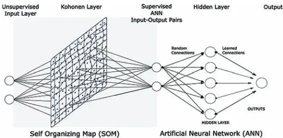
An alternative approach which has limited applications in drought forecasting is the optimal con-figuration of data-driven models in an ensemble with Kohonen’s self-organizing map (SOM) (Kohonen, 1998; 2014). SOM is a popular neural network tool offering an unsupervised method of clustering the feature data set values (Kalteh, Hjorth, & Berndtsson, 2008; Nourani, Baghanam, Adamowski, & Kisi, 2014). SOM can be applied to simplify the input series by identifying the underlying trends in the fea-ture datasets to be modelled, thus reducing the need for an intact data series. The feafea-ture dataset is then constructed from the simple random sampling of each of the clusters (Wu, May, Dandy, & Maier, 2012; Wu, May, Maier, & Dandy, 2013). The implementation of SOM for training and testing data set selec-tion incidentally provides a means to manage time series staselec-tionarity and linearity issues, both of which reduce the efficacy of stochastic models for forecasting purposes in climate applications. Hence, the more deliberate selection of training and testing data sets through SOM offers a convenient and effective method to optimize the architecture and improve the performance of data-driven forecasting models.

Optimization of the features in model input data with a SOM using the neural network clustering and random sampling approach can assist modelers in creating robust and statistically consistent training, validating and testing of data sets. This can lead to high-performing and efficient data-driven models. Such model optimization attributes are highly desirable in drought management and drought forecasting decision-support tools.

Selection of Representative Feature Training Sets With Self-Organized Maps

BACKGROUND

The implementation of measured and timely responses for proper management of drought requires spatially and temporally refined information, which is difficult to access from raw model input data (Sayers, Yuanyuan, Moncrieff, Jianqiang, Tickner, Gang, & Speed, 2017). However, there is a great potential for drought models to determine the daily evolution of precipitation related events (Kaur, & Jothiprakash, 2013; Mohanbhai, & Kumar, 2016; Nastos, Paliatsos, Koukouletsos, Larissi, & Moustris, 2014). Forecasting techniques can support the precise determination of the onset and termination of drought events, the detection of any fluctuations in drought severity, and accordingly, provide the op-portunity for appropriate action in response to anticipated exacerbation on water resources.

In a large municipal region such as the city of Brisbane, classified as one of the largest councils in Australia by its population and household size (Sinnewe, Kortt, & Dollery, 2015), empirical appraisal of the affliction brought about by drought is necessary for water resource management and drought risk mitigation (Sayers, Yuanyuan, Moncrieff, Jianqiang, Tickner, Gang, & Speed, 2017). In the search for sustainable management measures, the Brisbane City Council (BCC) is also required to appropriately manage water resources whilst serving the interests of its community members spread over an area of

about 1367.0km2_{. The study region is important as severe droughts have previously inflicted significant}

economic costs to Brisbane region, partly due to reactive large-scale infrastructure investments, which were relegated to expensive post-drought stranded assets (White, Turner, Chong, Dickinson, Cooley, & Donnelly, 2016). As a broader example, water restrictions imposed by local councils in response to severe drought conditions have been previously estimated to cost Australia up to a billion dollars per year (Radcliffe, 2015). Therefore, development of optimal models for drought forecasting is paramount for the future drought management of.

Informed decision-making and more measured approaches to the management of drought requires access to spatially and temporally refined information. A significant potential for the management of water resources exists in the predictive ability of hydrologists to forecast the daily evolution of drought parameters. This enables them to…, detect the onset and termination of drought events, the fluctuations in the drought severity, and accordingly, to provide the opportunity for actions to be taken in response to the anticipated exacerbation on water resources and relief of drought conditions. An operation of this magnitude thus requires precise and accurately forecasted drought parameters to inform decision-makers in the lead-up to, and through the duration of, drought conditions as has been experienced in recent history. Consequently, a predictive model communicating the evolution of drought parameters at short-term periods (e.g. daily time scales) presents an advantage to hydrologists for detecting and quantifying drought events, and for the development of early warning systems.

Selection of Representative Feature Training Sets With Self-Organized Maps

Various approaches used to model and predict drought behaviour exist in current literature. Data-driven models, such as Artificial Neural Networks (ANN), are valued for their demonstrated ability to detect and mimic non-formulated patterns in feature data (Elshorbagy, Corzo, Srinivasulu, & Solomatine, 2010). ANN have been recognized for their skill in forecasting the nonlinear inter- and intra-seasonal fluctuations in climate variables (Abbot, & Marohasy, 2012; Hosseini-Moghari, & Araghinejad, 2015; Tiwari, Adamowski, & Adamowski, 2016). Another commonly appraised approach to hydrological time series modeling is the classical linear stochastic Autoregressive Integrated Moving Average (ARIMA) model. Existing studies have demonstrated superior performance of ARIMA models over other statistical models used in short-term forecasting of hydrological time series (Abbot, & Marohasy, 2012; Hosseini-Moghari, & Araghinejad, 2015; Mishra, & Desai, 2005; Tiwari, Adamowski, & Adamowski, 2016). Both ANN and ARIMA are often considered as baseline models for predicting hydrological time series.

In this research, we propose a forecasting model for daily EDI using an ANN model for the City of Brisbane, Australia. We then incorporate the Kohonen’s SOM as an optimization tool for the ANN model and compare the performance with classical stochastic time series modeling techniques based on a standalone ARIMA model. SOM ensemble models offer the advantage of using statistically consistent data sets to build the ANN models, in addition to having time series stationarity issues removed, and managing non-continuous data sets, such as those disrupted by collection errors.

MATERIALS AND METHODS

Study Area and Climate Data

Daily precipitation data required to calculate the EDI were obtained from the Queensland Government Environmental Protection Agency (SILO) patched point values for specific stations (Jeffrey, S. J., Carter, Moodie, & Beswick, 2001). The data selected for this study is Amberley Authorised Maintenance Organisation (AMO) station within the vicinity of Wivenhoe Dam (White, Turner, Chong, Dickinson, Cooley, & Donnelly, 2016). The development of a predictive model for this site is appealing as the dam is a major water source for the City of Brisbane and sustainable measures for water resources need to be implemented in the face of drought conditions. The daily precipitation data were obtained for January 2017 from the SILO database at www.longpaddock.qld.gov.au/silo (Jeffrey, Carter, Moodie, & Bes-wick, 2001). This site was also selected based on the quality of the data, being a long time series with few missing values, to compare the veracity of the proposed models. Statistics capturing the nature of precipitation trends are provided in Table 1.

For this analysis, only data from 1970 to 2016 is being considered, where the earliest data in this set coincides with the onset of the first major drought affecting eastern Australia as identified in Mpelasoka et al. (2008).

Selection of Representative Feature Training Sets With Self-Organized Maps

Effective Drought Index (EDI)

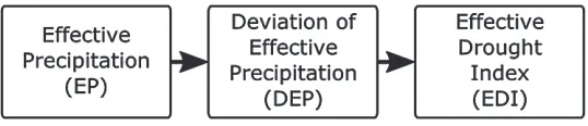
A concise overview of the EDI is presented here but readers can refer to the original work of Byun et al. (1999) for more refined detail. Figure 1 shows a summary schematic of how the EDI was calculated.

Based on daily precipitation data, the effective precipitation (EP) per day was calculated in terms of the depletion of daily water resources (Byun, & Wilhite, 1999), where:

EP = P

n

m m n

n D

=

=

∑

∑

    



     1 1

In the EP calculation, D is the duration of summation over an annual cycle (365 days), which is the most common precipitation cycle worldwide (Byun & Wilhite, 1999). The deviation of effective precipitation from the climatological mean (i.e., DEP) is the deficit of stored water quantity from the climatological mean (base period). It follows that:

DEP =EP MEP -

Note that MEP is the mean of each calendar day’s EP based on the 30-year baseline data series. The MEP has the potential to be affected by a strong daily variation in precipitation, and is therefore not helpful for practical use. As such, a 5-day running mean is normally applied (Byun & Wilhite, 1999) to smooth the trends.

EDI = DEP

DEP

SD( )

where SD(DEP) is the standard deviation of each calendar day’s EP on the 30-year baseline period.

Table 1. Study area climate statistics

Station,

BOM ID Location Elevation (m)

Climatological Precipitation, P (mm day-1₎

Mean Min Max Std. Dev.

Amberley AMO ID

40004 152.71

o_E,

-27.63o_S 24 2.30 0 240 8.54

Selection of Representative Feature Training Sets With Self-Organized Maps

Following these calculations, the EDI produces daily standardized values of water deficits relative to the base period. These have been interpreted as measures of severity of drought with nearly normal conditions (-1> EDI >1), moderate drought (-1.5> EDI ≥ 1), severe drought (-2 > EDI ≥ -1.5), and extreme drought EDI ≤ -2 (Morid, Smakhtin, & Moghaddasi, 2006).

Auto-Regressive Moving Average (Stochastic) Model

As commonly used representations of hydrological time series, stochastic models have been proven as systematic characterizations of time series for past, current and future trends in the data. Generally, stochastic models consist of autoregressive (AR), integrated (I) and moving average (MA) components of varying denominations, which may be identified in seasonal and/or non-seasonal occurrences (Box, Jenkins, Reinsel, & Ljung, 2015).

The general form of the seasonal ARIMA (or SARIMA) model is:

ARIMA (p, d, q) (P,D,Q)_S

which is the product of polynomials derived from:

• Non-seasonal autoregressive AR(p), relating the current value of the time series to past values of order p.

• Non-seasonal moving average MA(q), relating to past forecast errors of order q. • Differencing d, to adjust for non-seasonal non-stationarity.

• Seasonal autoregressive AR(P), relating the current value of the time series to regular (period S) past values of order P.

• Seasonal (period S) moving average MA(Q) relating to regular (period S) past forecast errors of order Q.

• Differencing D, to adjust for seasonal (period S) non-stationarity.

Requirements for using linear ARIMA models is that the time series is free of any deterministic structures such as pulses, level shifts, local time trends and seasonal pulses (Harvey, Jan Koopman, & Penzer, 1999). The assumptions of the ARIMA models also stipulate that the series has constant error variance and that the parameters of the proposed model remain constant over the course of time.

The most appropriate ARIMA model may be determined through three stages of model fitting: identification, estimation and diagnostic check (Box, Jenkins, Reinsel, & Ljung, 2015). The first stage, which is the selection of the set of more appropriate models, is achieved by examining the autocorrela-tion funcautocorrela-tion (ACF) and partial autocorrelaautocorrela-tion funcautocorrela-tion (PACF) distribuautocorrela-tions of the original time series of the daily EDI. The best model is recommended based on the combined testing for minimum values of Akaike Information Criterion (AIC) and Schwarz Bayesian Criterion (SBC), also called Bayesian Information Criterion (BIC) (Mishra, & Desai, 2005).

For AIC (Akaike, 1974) the mathematical formulation is defined by:

Selection of Representative Feature Training Sets With Self-Organized Maps

and the mathematical formulation for the BIC (Schwarz, 1978) is defined by:

BIC =m ln(n) - 2 log L

Artificial Neural Network (ANN) Model

The ANN model has been extensively researched in many meteorological applications and may be con-sidered for producing a standard baseline set of predictions. ANN requires iterative tuning of parameters to develop a proposed network architecture and may not always produce a global solution. Mathemati-cally, the ANN algorithm can be written as (Deo, R. C., & Şahin, 2015a; 2015b):

y x( )=

F

(

∑

)

where x_i(t) = feature variable(s) in discrete time space t, y(x) = forecasted EDI in test data set, L =

hid-den neurons determined iteratively, ω_i (t) = weight that connects the ith _{neuron in the input layer, b =}

neuronal bias and F(.)is the hidden transfer function.

A three-layer multilayer feedforward (MLFF) was developed, trained and tested for estimating EDI from the significant inputs. The network is trained from a portion of the data’s observed inputs and output or target vector set. During the training stage, the weights and biases of the data are adjusted to minimise the error between the target and the predicted output. The proposed three-layer feed-forward model uses features EDI_t, EDI_t-1, .., EDI_t-n which are the previous lagged observations. The output EDI_t+L provides the forecast for the future value where L is the lead time, with the preceding EDI value being considered in this study.

The training algorithm used, Levenberg-Marquardt, is a variant of the Newton Raphson method and relies on having a quality initial estimate of the hidden layer parameters for ultimate success. Poor initial conditions may result in an algorithm that has slow and difficult training, and does not produce a unique global solution.

As noted by Deo, R. C., Byun, et al. (2016), traditional models such as ANN have also been criticized for their poor handling of stochastic nature of meteorological processes. The implementation of wavelets in pre-processing of the training data enabled the capturing of underlying frequency information, thus dramatically improving the performance of the model (as seen by the analysis of the test data statistics).

Predictive Model Development

Selection of Representative Feature Training Sets With Self-Organized Maps

Typically, these subsets are defined by data splitting operation at arbitrary points. An example is 80% for model development (60% training, 20% validating) and 20% for? testing, based on the commonly and diversely applied phenomena known as the Pareto principle for model development and evaluation.

Maier et al. (2000) suggest using a SOM to ensure that training, validating and testing data sets are representative of the same population and demonstrate similar statistical properties. This results in/can result in improved quality of the characterizations and predictions.

During intelligent learning processes, neurons in the network enhance their sensitivity to detect changes in the behaviour of feature sets. A data-intensive approach uses classification to create separate classes of data sharing similar properties (Kalteh, Hjorth, & Berndtsson, 2008; Maier, Jain, Dandy, & Sudheer, 2010). An unsupervised method is Kohonen’s SOM, which separates the feature set’s values into a predetermined number of denominations using clustering.

The simple random sampling of data from each cluster also diminishes the risk of over training, while still demonstrating the ability to capture the nature of the feature sets considered (Figure 2).

The EDI values are classified based on the clustering of lags of the daily EDI values using SOM.

The sequence of EDI values forms a series

{ }

broadcast to a set of models Mi, of which Mc fits the best. The values of the other sequences

{

}

of n-dimensional real vectors are iteratively computed approximations to the model m_i, with i denoting

the index of the node.

The SOM algorithm mechanisms are based on the convergence of the following function, which would produce a set of ordinal values for the model,

m_i(t + =1) m_i( )t +h t_ci( )[ ( )mt −m_i( )]t

where h t_ci( ) is the neighborhood function, performing the defining role in the self-organization process.

This function resembles kernel-based smoothing processes, except in the SOM, c is the index of a

nominated node (winner) in the array with the model m_c(t) determined to have minimum Euclidean

distance from x(t):

Selection of Representative Feature Training Sets With Self-Organized Maps

c=arg min_i

{

}

A commonly applied neighbourhood function is:

h t c,i

t

ci( )= _{( )}



  



   α

σ

(t) exp -sqdist( ) 2 2

where α(t) < 1 is a monotonic (e.g., hyperbolically, exponentially, or piecewise linearly) decreasing scalar function of t, sqdist(c, i) is the square of the geometric distance between the nodes c and i in the array, and σ(t) is another monotonically decreasing function of t, respectively. According to Kohonen (2014), the true mathematical form of σ(t) is not crucial, while the value is on the order of 20% of the longer dimension of the SOM array which is then gradually reduced after several thousand iterations.

Currently there is no standard for determining the optimum size of the Kohonen layer for unsuper-vized training, and hence the Kohonen layer dimensions adopted by Bowden et al. (2002) were used, that is 10 rows x 10 columns grid clusters, to find a balance between computation time and maximise data dispersion.

This was achieved using MATLAB’s in-built selforgmap function, utilizing the default settings for

all other input parameters. Two trials were performed, with up to 120 and 150 data values respectively (randomly selected without replacement) being selected from each of the resulting 100 clusters and assigned as training, validating or testing data subsets. A visual quality check was made possible by

inspecting the distribution of samples from each cluster using MATLAB’s plotsomhits function.

Performance Evaluation

In the absence of a standard evaluation framework to measure the efficacy of all simulations, Dawson et al. (2007) suggests that a variety of indices be used. Model performance metrics typically present assessments of bias and variability.

There are common model accuracy assessment metrics (Legates, & McCabe, 1999) which have been widely adopted to determine the performance of a model. Expressions of the formulation for each were

customized to suit EDI data driven forecasting by Deo, R. C., Tiwari, et al. (2016) where EDI_o and EDI_p

are the observed and forecasted ith _{EDI which are then averaged over the baseline period (1971-2000),}

N is the number of data points, and EDI_opeak _{and EDI}

ppeak are the peak EDI values in observed and

fore-casted sets, respectively.

• Coefficient of Determination (r2₎

Selection of Representative Feature Training Sets With Self-Organized Maps

r2 ₌ EDI EDI EDI EDI

EDI EDI

o,i o,i p,i p,i

o,i o,i −

(

)

(

)

(

)

∑

∑

∑

∑

(

)

= EDIp,i EDIp,i 2

1

2

i N

• Wilmott’s Index of Agreement (d)

In Wilmott’s Index of agreement, the maximum possible sum of squared simulation error (numera-tor) is compared to the variance of the observation data set (denomina(numera-tor). Issues with this metric lie in the squaring of errors before adding them, which will magnify skew and extreme data significantly and overweigh the influence of these errors.

d = 1 1

2

1

2

- EDI EDI

EDI EDI

o,i p,i o,i o,i −

(

)

(

)

∑

∑

, 0 ≤ d ≤1

• Nash-Sutcliffe Coefficient

Nash-Sutcliffe coefficient, E_NS, is an alternative metric for goodness of fit which is sensitive to additive and proportional discrepancies between the simulated and observed values (Legates, & McCabe, 1999)

E_NS = 1 1

2

- EDI EDI

EDI EDI EDI EDI

o,i p,i

p,i o,i o,i o,i −

(

)

(

)

∑

i==

∑

N , -∞ ≤ ENS ≤1

• Percentage Peak Deviation (P_dv)

By quick inspection of P_dv, the presence and direction of bias in the model may be detected, with

positive P_dv and negative P_dv potentially indicating overestimate and underestimate biases respectively.

Values of P_dv close to zero could potentially indicate either a well-fitting model or an aggregately

neu-tral model, where the peak deviations are cumulatively balanced out, and hence this performance index should not be used in isolation.

P_DV = 100

1

EDI EDI

Selection of Representative Feature Training Sets With Self-Organized Maps

• Root Mean Square Error (RMSE) and Mean Absolute Error (MAE)

Both RMSE and MAE quantify the average deviation of simulated values from the observed values. MAE gives equal weighting the deviations, whereas the RMSE amplifies errors proportionally to their size through the squaring operation. Hence this recommends MAE to situations where the error has a uniform distribution and the RMSE to normally shaped (Gaussian) approximating error distributions (Chai, & Draxler, 2014)

RMSE = 1 ₁ 2

N i

N

EDI_p,i− EDI_o,i

(

)

=

∑

MAE = 1 ₁

N i

N

EDI_p,i− EDI_o,i

=

∑

Due to the squaring mechanism in their respective formulations, r2_{, E}

NS and RMSE are sensitive to

the effects of extreme values.

RESULTS AND DISCUSSION

An initial inspection of the time series of the EDI for Amberley AMO (at SILO station number 40004) reveals the presence of several uncharacteristic and influential pulses. These spikes each result in EDI>4 and coincide with the timing of significant precipitation events and regional flooding.

ARIMA model selection:

An inspection of AIC and BIC values associated with each ARIMA daily EDI model for minimum values is presented in Table 2. The corresponding ACF and PACF is provided in Figure 3.

Despite the high likelihood of annually reoccurring seasonal variations being present in the time series, a resolution coarser than daily units would be needed for their precise detection over the duration of a year. Hence, no seasonal differencing will be applied.

Each model has been trained, validated and tested individually on model-specific data subsets sourced from 1 January 1970 and 31 December 2015. A secondary independent subset (1 Jan 2016 – 8 Jan 2017) was reserved for comparative testing between the different models.

An inspection of the distribution statistics for the aforementioned subsets (Table 3 and Table 4) reveals a notable difference. When using the 60:20:20 chronologically segmented approach, the training, vali-dating and testing distributions convey inconsistent characteristics, resulting in a less optimally trained model. In contrast, the SOM ensemble ANN models use random sampling from the entire time series

Table 2. Comparison of AIC and SBC for selected candidate models

Model AIC BIC

Selection of Representative Feature Training Sets With Self-Organized Maps

producing highly representative consistent training and testing data sets. This demonstrates the disparity between training and testing data sets that potentially occurs when data is arbitrarily split.

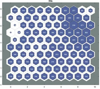
The SOM ANN application to the data set is further tested to include the bulk of the data available, by considering larger training, validating and testing data sets, to include 4593 values in each. Figure 4 provides a visualization of the distribution of the samples across the SOMs, which indicates a good spread of the data between the clusters.

While these metrics measure the individual model’s capacity to capture and replicate the nature of the corresponding data sets’, shown in Table 3 and 4, another test is required to equitably compare them against each other. Hence, each model has also been tested on an independent and previously untested common data subset (Table 5), with the results presented in Table 7.

At first inspection of the model performance metrics presented (Table 6), there appears to be little discernible difference between the models’ performances. The ARIMA model and the lag driven ANN implemented to provide a direct comparison to the ARIMA model are deeply connected to the individual linear effects of incremented values for the modelled variable, and both demonstrate an affinity with the similarly lagged value dependent nature of the daily EDI.

Generally, all models performed strongly, with high correlations between actual and predicted EDI. This is highly complementary to the optimized sampling methods used in the development of the SOM ensemble models which are training on less than half of the data used in the traditional ARIMA and ANN models.

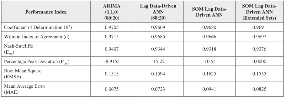
These performances are repeated for the second verification set (Table 7) which exposes the models to a previously reserved feature data from 1 January 2016 – 8 January 2017.

Overall these results demonstrate the strong potential for SOM to overcome issues with available data, and to develop a representative training set from a minimum number of samples.

Selection of Representative Feature Training Sets With Self-Organized Maps

Figure 4. An examination of the distribution of the net simulated samples using MATLAB’s plotsomhits for the extended SOM data sets

Table 3. Statistics of the Lagged EDI Training, Testing, and Validation Data Sets (arbitrary chronologi-cal 60:20:20 division) for ANN and ARIMA

Sample Size Mean _DeviationStandard Max Min IQR

Input: EDIt-1

Training 10073 0.13 1.05 8.70 -2.14 1.29 Validating 3358 -0.57 0.55 2.30 -1.76 0.68 Testing 3358 0.21 1.02 6.76 -1.94 0.10

Output EDIt

Selection of Representative Feature Training Sets With Self-Organized Maps

The second verification data set used produced some lower metrics (Table 7) than the first set (Table 6) for the SOM models as the new regions of data demonstrated unfamiliar behaviour to the model’s expectations. Understandably, there can be no assurance of the predictive capability of data-intensive models under untried circumstances. However, as Bowden et al. (2002) suggests SOM-aided models may overcome this shortcoming by implementing a sporadic retraining regime for the model.

FUTURE RESEARCH DIRECTION

Further enhancement of the SOM methodology would involve developing an algorithm which helps to decide the optimal number of clusters based on smoothing the distribution of samples about the SOM.

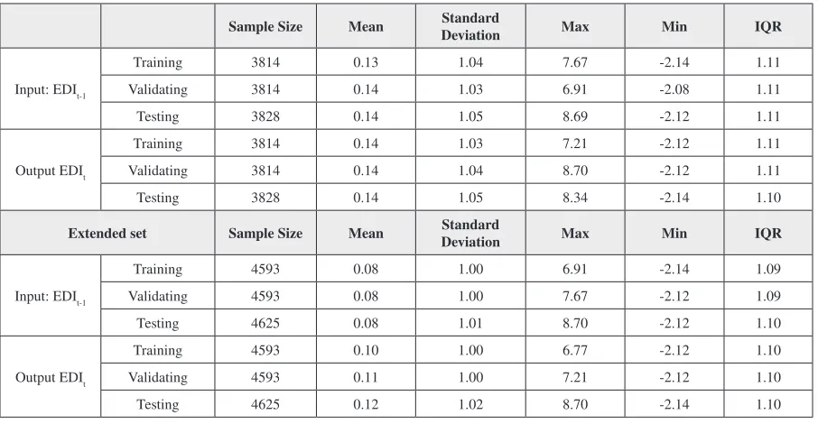
Table 4. Statistics of the Lagged EDI Training, Testing, and Validation Data Sets (Data Divided Using a SOM using an extended data set for testing performance alongside the ARIMA models. Note that the output EDI is not used in the self-organizing mapping process, but shown here as a comparison between the statistics of the subsets.

Sample Size Mean DeviationStandard Max Min IQR

Input: EDIt-1

Training 3814 0.13 1.04 7.67 -2.14 1.11 Validating 3814 0.14 1.03 6.91 -2.08 1.11 Testing 3828 0.14 1.05 8.69 -2.12 1.11

Output EDIt

Training 3814 0.14 1.03 7.21 -2.12 1.11 Validating 3814 0.14 1.04 8.70 -2.12 1.11 Testing 3828 0.14 1.05 8.34 -2.14 1.10

Extended set Sample Size Mean _DeviationStandard Max Min IQR

Input: EDIt-1

Training 4593 0.08 1.00 6.91 -2.14 1.09 Validating 4593 0.08 1.00 7.67 -2.12 1.09 Testing 4625 0.08 1.01 8.70 -2.12 1.10

Output EDIt

Training 4593 0.10 1.00 6.77 -2.12 1.10 Validating 4593 0.11 1.00 7.21 -2.12 1.10 Testing 4625 0.12 1.02 8.70 -2.14 1.10

Table 5. Statistics of the common data subset (1 Jan 2016 – 8 Jan 2017) used for testing on all models to allow a fair comparison of models

Sample Size Mean DeviationStandard Max Min IQR

Input EDIt-1

Common

Selection of Representative Feature Training Sets With Self-Organized Maps

On a broader scale, further investigation is warranted to determine the cost in performance and ef-ficiency that is associated with using poorly considered data sets for training and validating data-driven models.

CONCLUSION

Daily drought forecast models provide insightful information into the evolution of precipitation deficit events; this allows policy makers for municipals such as the Brisbane City Council to take appropriate management actions. Typically, the focus of model development involves the mechanisms of the model itself, rather than considering the simple optimizations that may be made possible through inspection and strategic selection of data.

Table 6. Performance indices for the respective models, each using customized test data sets for assess-ment. Values reported here will indicate individual model performance only and cannot be compared across columns, to other models.

Performance Index ARIMA (1,1,0) (80:20)

Lag Data-Driven ANN (80:20)

SOM Lag Data- Driven ANN

SOM Lag Data- Driven ANN (Extended Sets)

Coefficient of Determination (R2_{) 0.9841 0.9830 0.9878 0.9847}

Wilmott Index of Agreement (d) 0.9789 0.9776 0.9826 0.9779 Nash-Sutcliffe

(ENS) 0.9680 0.9663 0.9757 0.9664

Percentage Peak Deviation (PDV) -3.3082 4.2622 0.0055 -0.0000

Root Mean Square

(RMSE) 0.1823 0.1871 0.1640 0.1837 Mean Average Error

(MAE) 0.0761 0.0780 0.0766 0.0781

Table 7. Performance indices for the respective models, using a common test data set for assessment (1 Jan 2016 – 8 Jan 2017). Values reported here may be used in an across column model comparison.

Performance Index ARIMA (1,1,0) (80:20)

Lag Data-Driven ANN (80:20)

SOM Lag Data- Driven ANN

SOM Lag Data- Driven ANN (Extended Sets)

Coefficient of Determination (R2_{) 0.9705 0.9669 0.9680 0.9691}

Wilmott Index of Agreement (d) 0.9715 0.9685 0.9666 0.9697 Nash-Sutcliffe

(ENS) 0.9407 0.9344 0.9318 0.9376

Percentage Peak Deviation (PDV) -8.9155 -15.22 -10.54 0.0000

Root Mean Square

(RMSE) 0.1515 0.1594 0.1625 0.1555 Mean Average Error

Selection of Representative Feature Training Sets With Self-Organized Maps

SOM-ANN ensemble models demonstrate competitive predictive performance for daily EDI values to those produced by ARIMA models. Aside from computational costs, the additional benefit lies in the SOM pre-processed ANN performing robustly and competitively with reduced data or incomplete data sets.

The best measurement of the quality of the data-interrogative model relies on having training data sets which resemble the testing data set, rather than using the widely accepted arbitrary chronological division selection methods in literature. Hence self-organizing mapping techniques which use unsuper-vised clustering and subsequent sampling from those clusters to create training and testing sets for model development is a rational choice.

REFERENCES

Abbot, J., & Marohasy, J. (2012). Application of artificial neural networks to rainfall forecasting in

Queensland, Australia. Advances in Atmospheric Sciences, 29(4), 717–730. doi:10.100700376-012-1259-9

Akaike, H. (1974). A new look at the statistical model identification. IEEE Transactions on Automatic

Control, 19(6), 716–723. doi:10.1109/TAC.1974.1100705

Bowden, G. J., Maier, H. R., & Dandy, G. C. (2002). Optimal division of data for neural network models

in water resources applications. Water Resources Research, 38(2), 2-1–2-11. doi:10.1029/2001WR000266

Box, G. E., Jenkins, G. M., Reinsel, G. C., & Ljung, G. M. (2015). Time series analysis: forecasting

and control. John Wiley & Sons.

Byun, H.-R., & Wilhite, D. A. (1999). Objective quantification of drought severity and duration. Journal

of Climate, 12(9), 2747–2756. doi:10.1175/1520-0442(1999)012<2747:OQODSA>2.0.CO;2

Cai, W., Borlace, S., Lengaigne, M., Van Rensch, P., Collins, M., Vecchi, G., ... Wu, L. (2014).

Increas-ing frequency of extreme El Niño events due to greenhouse warmIncreas-ing. Nature Climate Change, 4(2),

111–116. doi:10.1038/nclimate2100

Chai, T., & Draxler, R. R. (2014). Root mean square error (RMSE) or mean absolute error

(MAE)?–Ar-guments against avoiding RMSE in the literature. Geoscientific Model Development, 7(3), 1247–1250.

doi:10.5194/gmd-7-1247-2014

Dawson, C. W., Abrahart, R. J., & See, L. M. (2007). HydroTest: A web-based toolbox of evaluation

metrics for the standardised assessment of hydrological forecasts. Environmental Modelling & Software,

22(7), 1034–1052. doi:10.1016/j.envsoft.2006.06.008

Dayal, K., Deo, R. C., & Apan, A. A. (2017). Drought Modelling Based on Artificial Intelligence and Neural Network Algorithms: A Case Study in Queensland, Australia. In Climate Change Adaptation in Pacific Countries (pp. 177-198). Springer.

Deo, R. C., Byun, H., Adamowski, J., & Kim, D. (2014). Diagnosis of flood events in Brisbane

Selection of Representative Feature Training Sets With Self-Organized Maps

Deo, R. C., Byun, H.-R., Adamowski, J. F., & Begum, K. (2016). Application of effective drought index

for quantification of meteorological drought events: A case study in Australia. Theoretical and Applied

Climatology, 1–21.

Deo, R. C., Kisi, O., & Singh, V. P. (2017). Drought forecasting in eastern Australia using

multivari-ate adaptive regression spline, least square support vector machine and M5Tree model. Atmospheric

Research, 184, 149–175. doi:10.1016/j.atmosres.2016.10.004

Deo, R. C., & Şahin, M. (2015a). Application of the artificial neural network model for prediction of monthly standardized precipitation and evapotranspiration index using hydrometeorological

pa-rameters and climate indices in eastern Australia. Atmospheric Research, 161, 65–81. doi:10.1016/j.

atmosres.2015.03.018

Deo, R. C., & Şahin, M. (2015b). Application of the extreme learning machine algorithm for the

pre-diction of monthly Effective Drought Index in eastern Australia. Atmospheric Research, 153, 512–525.

doi:10.1016/j.atmosres.2014.10.016

Deo, R. C., Tiwari, M. K., Adamowski, J. F., & Quilty, J. M. (2016). Forecasting effective drought index

using a wavelet extreme learning machine (W-ELM) model. Stochastic Environmental Research and

Risk Assessment, 1–30.

Djerbouai, S., & Souag-Gamane, D. (2016). Drought forecasting using neural networks, wavelet neural

networks, and stochastic models: Case of the Algerois Basin in North Algeria. Water Resources

Man-agement, 30(7), 2445–2464. doi:10.100711269-016-1298-6

Ebi, K., Mearns, L., & Nyenzi, B. (2003). Weather and climate: changing human exposures. In A. J.

McMichael, D. H. Campbell-Lendrum, C. F. Corvalan, K. L. Ebi, A. Githeko, & ... (Eds.), Climate

Change and Health: Risks and Responses. Geneva: World Health Organization.

Elshorbagy, A., Corzo, G., Srinivasulu, S., & Solomatine, D. (2010). Experimental investigation of the predictive capabilities of data driven modeling techniques in hydrology-Part 1: Concepts and

methodol-ogy. Hydrology and Earth System Sciences, 14(10), 1931–1941. doi:10.5194/hess-14-1931-2010

Guttman, N. B. (1998). Homogeneity, data adjustments and Climatic Normals. National Climatic Data

Center.

Harvey, A., Jan Koopman, S., & Penzer, J. (1999). Messy time series. In Messy Data (pp. 103–143).

Emerald Group Publishing Limited. doi:10.1108/S0731-9053(1999)0000013007

Hosseini-Moghari, S. M., & Araghinejad, S. (2015). Monthly and seasonal drought forecasting using

statistical neural networks. Environmental Earth Sciences, 74(1), 397–412. doi:10.100712665-015-4047-x

Jeffrey, S. J., Carter, J. O., Moodie, K. B., & Beswick, A. R. (2001). Using spatial interpolation to

con-struct a comprehensive archive of Australian climate data. Environmental Modelling & Software, 16(4),

309–330. doi:10.1016/S1364-8152(01)00008-1

Kalteh, A. M., Hjorth, P., & Berndtsson, R. (2008). Review of the self-organizing map (SOM) approach

in water resources: Analysis, modelling and application. Environmental Modelling & Software, 23(7),

Selection of Representative Feature Training Sets With Self-Organized Maps

Kaur, H., & Jothiprakash, V. (2013). Daily precipitation mapping and forecasting using data driven

techniques. International Journal of Hydrology Science and Technology, 3(4), 364–377. doi:10.1504/

IJHST.2013.060337

Kohonen, T. (1998). The self-organizing map. Neurocomputing, 21(1), 1–6.

doi:10.1016/S0925-2312(98)00030-7

Kohonen, T. (2014). MATLAB Implementations and Applications of the Self-organizing Map. Helsinki:

Unigrafia Oy.

Legates, D. R., & McCabe, G. J. Jr. (1999). Evaluating the use of “goodness‐of‐fit” measures in hydrologic and

hydroclimatic model validation. Water Resources Research, 35(1), 233–241. doi:10.1029/1998WR900018

Maier, H. R., & Dandy, G. C. (2000). Neural networks for the prediction and forecasting of water

re-sources variables: A review of modelling issues and applications. Environmental Modelling & Software,

15(1), 101–124. doi:10.1016/S1364-8152(99)00007-9

Maier, H. R., Jain, A., Dandy, G. C., & Sudheer, K. P. (2010). Methods used for the development of neural networks for the prediction of water resource variables in river systems: Current status and future

directions. Environmental Modelling & Software, 25(8), 891–909. doi:10.1016/j.envsoft.2010.02.003

Masinde, M., & Bagula, A. (2011). The role of ICTS in quantifying the severity and duration of climatic

variations—Kenya’s case. Paper presented at the Kaleidoscope 2011: The Fully Networked Human?-Innovations for Future Networks and Services (K-2011).

Mishra, A., & Desai, V. (2005). Drought forecasting using stochastic models. Stochastic Environmental

Research and Risk Assessment, 19(5), 326–339. doi:10.100700477-005-0238-4

Mishra, A. K., & Singh, V. P. (2010). A review of drought concepts. Journal of Hydrology (Amsterdam),

391(1), 202–216. doi:10.1016/j.jhydrol.2010.07.012

Mohanbhai, K. P., & Kumar, P. (2016). Application of Artificial Neural Networks for Short Term Rainfall

Forecasting. Academic Press.

Morid, S., Smakhtin, V., & Moghaddasi, M. (2006). Comparison of seven meteorological indices for

drought monitoring in Iran. International Journal of Climatology, 26(7), 971–985. doi:10.1002/joc.1264

Mpelasoka, F., Hennessy, K., Jones, R., & Bates, B. (2008). Comparison of suitable drought indices for

climate change impacts assessment over Australia towards resource management. International Journal

of Climatology, 28(10), 1283–1292. doi:10.1002/joc.1649

Nastos, P., Paliatsos, A., Koukouletsos, K., Larissi, I., & Moustris, K. (2014). Artificial neural networks

modeling for forecasting the maximum daily total precipitation at Athens, Greece. Atmospheric Research,

144, 141–150. doi:10.1016/j.atmosres.2013.11.013

Nelson, M., Hill, T., Remus, W., & O’Connor, M. (1999). Time series forecasting using neural

net-works: Should the data be deseasonalized first? Journal of Forecasting, 18(5), 359–367. doi:10.1002/

Selection of Representative Feature Training Sets With Self-Organized Maps

Nourani, V., Baghanam, A. H., Adamowski, J., & Kisi, O. (2014). Applications of hybrid

wavelet–Ar-tificial Intelligence models in hydrology: A review. Journal of Hydrology (Amsterdam), 514, 358–377.

doi:10.1016/j.jhydrol.2014.03.057

Nury, A. H., Hasan, K., & Alam, M. J. B. (2017). Comparative study of wavelet-ARIMA and wavelet-ANN

models for temperature time series data in northeastern Bangladesh. Journal of King Saud

University-Science, 29(1), 47–61. doi:10.1016/j.jksus.2015.12.002

Radcliffe, J. C. (2015). Water recycling in Australia–during and after the drought. Environmental

Sci-ence. Water Research & Technology, 1(5), 554–562. doi:10.1039/C5EW00048C

Sayers, P. B., Yuanyuan, L., Moncrieff, C., Jianqiang, L., Tickner, D., Gang, L., & Speed, R. (2017).

Strategic drought risk management: Eight ‘golden rules’ to guide a sound approach. International Journal

of River Basin Management, 1-17.

Schwarz, G. (1978). Estimating the dimension of a model. Annals of Statistics, 6(2), 461–464. doi:10.1214/

aos/1176344136

Shirmohammadi, B., Vafakhah, M., Moosavi, V., & Moghaddamnia, A. (2013). Application of several

data-driven techniques for predicting groundwater level. Water Resources Management, 27(2), 419–432.

doi:10.100711269-012-0194-y

Sinnewe, E., Kortt, M. A., & Dollery, B. (2015). Is biggest best? a comparative analysis of the financial

viability of the Brisbane City Council. Australian Journal of Public Administration.

Stern, H., De Hoedt, G., & Ernst, J. (2000). Objective classification of Australian climates. Australian

Meteorological Magazine, 49(2), 87–96.

Tiwari, M., Adamowski, J., & Adamowski, K. (2016). Water demand forecasting using extreme learning

machines. Journal of Water and Land Development, 28(1), 37–52. doi:10.1515/jwld-2016-0004

White, S., Turner, A., Chong, J., Dickinson, M., Cooley, H., & Donnelly, K. (2016). Managing drought:

Learning from Australia. Academic Press.

Wu, W., May, R., Dandy, G. C., & Maier, H. R. (2012). A method for comparing data splitting approaches

for developing hydrological ANN models. International Environmental Modelling and Software Society (iEMSs).

Wu, W., May, R. J., Maier, H. R., & Dandy, G. C. (2013). A benchmarking approach for comparing

data splitting methods for modeling water resources parameters using artificial neural networks. Water

Resources Research, 49(11), 7598–7614. doi:10.1002/2012WR012713

Zargar, A., Sadiq, R., Naser, B., & Khan, F. I. (2011). A review of drought indices. Environmental

Reviews, 19, 333-349.

Zhang, G. P. (2003). Time series forecasting using a hybrid ARIMA and neural network model.

Neuro-computing, 50, 159–175. doi:10.1016/S0925-2312(01)00702-0

Zhang, G. P., & Qi, M. (2005). Neural network forecasting for seasonal and trend time series. European