Dimension-deficient channel estimation of hybrid beamforming based on compressive sensing

Dimension-Deficient Channel Estimation

of Hybrid Beamforming Based on

Compressive Sensing

YU XIAO 1, (Student Member, IEEE), YAFENG WANG 1, (Senior Member, IEEE), AND WEI XIANG 2, (Senior Member, IEEE)

1_{Key Laboratory of Universal Wireless Communications, Ministry of Education, Beijing University of Posts and Telecommunications, Beijing 100876, China} 2_{College of Science and Engineering, James Cook University, Cairns, QLD 4878, Australia}

Corresponding authors: Yafeng Wang (wangyf@bupt.edu.cn) and Wei Xiang (wei.xiang@jcu.edu.au)

This work was supported by the National Key Technology Research and Development Program of China under Grant 2017ZX03001012-003.

ABSTRACT Due to high hardware costs for digital beamforming, hybrid beamforming (HBF) is widely employed in millimeter-wave (mmWave) communications systems. However, the number of radio frequency chains in the analog part of HBF is far less than that of antennas, which causes a serious dimension-deficient problem. In order to overcome this problem, this paper proposes a compressive sensing algorithm using an adaptive overcomplete dictionary to estimate the sparse channel in the HBF-based mmWave system. The algorithm adaptively generates the dictionary by using the received signal to accurately reconstruct the mmWave channel. The simulation results are presented to demonstrate that the proposed algorithm outper-forms its traditional counterparts in terms of the normalized mean square error and the spectral efficiency.

INDEX TERMS Sparse channel estimation, hybrid beamforming, adaptive overcomplete dictionary, compressive sensing.

I. INTRODUCTION

In order to meet the explosive demands of user data growth, the current spectrum scarcity crisis needs to be addressed [1]–[3]. Thanks to abundant spectral resources, mmWave communications are widely studied in the fifth generation (5G) mobile networks. Although offloading data to mmWave spectra can improve channel capacity, it is not without sacrifices. Air is a highly absorptive dielectric with respect to the mmWave spectra, so the resulting path losses are very severe, thereby limiting the coverage of a base station [4]. However, mmWave has shorter wavelengths than the current LTE band, which means it is capable of packing more antennas in a limited physical space. The increased number of antennas will bring about more channel gains through the use of techniques such as precoding. Therefore, massive multiple-input multiple-output (MIMO) technology can be fully utilized in mmWave bands.

For the purpose of overcoming the shortcomings of mmWave communications and taking advantage of the gains brought by multiple antennas, digital beamforming (DBF) technology is widely considered. However, in the number of antennas, hardware costs become the main bottleneck

with the increase in massive MIMO. Then analog beam-forming (ABF) is adopted to reduce hardware costs, which evolves into HBF technology. HBF is adopted by 5G wire-less communication systems to achieve better beamforming gains. Because of the use of analog components, HBF usually cannot attain the same performance of DBF. Nevertheless, it is proved in [4] that HBF is able to achieve almost the same performance as DBF in terms of SE, when the num-ber of RF chains is twice as that of data streams or more. While the algorithm proposed in [4] focuses primarily on the single-user scenario. When extended to the scenario of multiple users, SE will decrease at low signal-to-noise ratios (SNRs). In [5], the algorithm is extended from the single-user scenario to the multi-user one, while it pro-poses a different HBF design method that can maximize system capacity. To address the problem of multiple users, a novel algorithm is proposed in [6]. The proposed HBF matrix for multiple users is not only superior in limited feedback and training overhead, but also helps achieve an excellent system performance. However, it is noted that the HBF performance in [6] is nearly equal to its DBF counter-part, only when data are transmitted with a single antenna.

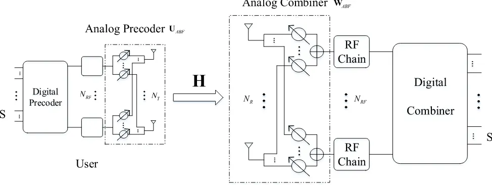
FIGURE 1. Block diagram of the mmWave communications system with full-connection HBF.

System coverage degrades with the increase in the number of channels.

To address the challenges of channel estimation (CE) in HBF, an adaptive algorithm is proposed to estimate the angle of arrival (AoA) and the angle of departure (AoD) for channel reconstruction in [7]. An algorithm is presented in lieu of the singular value decomposition (SVD) for channel estimation, which can reduce the computational complexity and the feed-back overhead [8]. In [9], an asymmetric beam search scheme is used to estimate the channel taking into account the sparsity of the mmWave channel. On one hand, this scheme employs CS to reduce the training overhead at the transmitter. On the other hand, the receiver utilizes exhaustive beam training to ensure a robust performance at low SNRs.

Different from the CS-based method to estimate the AoA

and AoD matrix of channel, Guo et al.[10] present a

two-dimensional multiple signal classification (2-D MUSIC) algorithm used in the beam space to estimate the directions of the mmWave channel. It is different from the conventional MUSIC algorithm used in the element space, which can only estimate one dimension (i.e. AoA or AoD) at a time and also does not consider beamforming. While it is stated in [10] that the beamspace MUSIC algorithm suffers from the problem of spectrum ambiguity, which means the quantized ABF may cause the miss match problem during the process of finding the extreme point of the directional spectrum. The 2-D MUSIC algorithm is also studied in [11], where an efficient 2-D direction-finding MUSIC algorithm based on the double polynomial root finding procedure is proposed to estimate the AoA and AoD jointly.

In most cases, the number of RF chains is far less than that of antennas. Therefore, the received signal does not contain full channel state information (CSI). This phenomenon, which is dubbed dimension-deficient, makes channel estimation in HBF different from conventional

channel estimation. In order to tackle the dimension-deficient challenge, this paper proposes a CS-based channel estimation algorithm for uplink single-user MIMO systems. Compared with conventional channel estimation methods, the proposed algorithm designs an adaptive overcomplete dictionary to improve the reconstruction probability at low SNRs, in an effort to reduce the NMSE.

Contribution:this paper proposes a dictionary-adaptive

compressive sensing channel estimation algorithm to over-come the dimension-deficient problem in HBF. Compared with conventional CS channel estimation methods in massive MIMO systems, the novelty of the proposed algorithm lies in the construction of an adaptive dictionary to deal with the dimension-deficient issue, improve the robustness against noise at low SNRs, minimize the NMSE of channel estima-tion, and achieve nearly identical SE.

Notation:X,xandxrepresent a matrix, vector and scalar, respectively. (∗)T, (∗)H, (∗)−1, (∗)†,vec(∗) andk∗k_F denote the transport, conjugate transport, inverse, pseudo-inverse, vectorize, and Frobenius norm of a matrix, respectively.⊗

indicates the Kronecker product operator.

This paper is organized as follows. SectionIIdescribes the

system and mmWave channel models. SectionIIIproposes

the CS-based channel estimation scheme to cope with the dimension-deficient challenge in HBF. SectionIVpresents the simulation results of the proposed algorithm, and com-pares them with those of the conventional channel estimation algorithms in [8], [10], and [18]. Finally, concluding remarks are drawn in SectionV.

II. SYSTEM MODEL

HBF is connected to every antenna, so all the antennas can be optimized jointly and the transceiver have a finer beam with full beamforming gains. On the other hand, each RF chain in partially connected HBF is connected to a subset of the antennas, so this structure has lower hardware complexity than its fully connected counterpart, while its array gain is lower and the beam width is rougher. Consequently, this paper chooses fully connected HBF as shown in Fig.1. Due to HBF being usually implemented on both uplink and downlink sides, we will only consider the uplink channel estimation at the gNB side for simplicity without loss of generality. The UE is equipped withNT antennas andNRF RF chains, while the gNB is equipped withNRantennas andNRF RF chains. It is noted that the numbers of RF chains are generally different for the UE and gNB. But this fact has no impact on the research under consideration in this paper, so it is assumed that the numbers of RF chains at the UE and gNB are the same. The number of RF chains should be far less than that of antennas, i.e.,NRF NR.

Considering the sparsity of the mmWave channel, the fol-lowing channel model that has be widely considered in the literature is adopted [6]–[9], [16]

H=

r NTNR

L

L

X

l=1

αlar θlr

aH_t θ_lt_,

(1)

whereLis the number of channel paths,αl ∼CN 0, σ_α2is

the channel gain,ar θlr

andat θlt

are the arrival steering and departure steering vectors, respectively.θ_ltandθ_lrare the azimuth angles of departure and arrival uniformly distributed

in [0,2π). Assuming the uniform linear arrays (ULA)

antennas, the steering vectors are shown as ar θ_lr =

1

√

NR

h

1,ej2λπdsin(θlr), . . . ,_ej(NR−1)2_λπdsin(θlr)

iT

andat θlt

₌

1

√

NT

h

1,ej2λπdsin(θlt), . . . ,_ej(NT−1)2_λπdsin(θlt)

iT

, where d =

λ

2 andλis the carrier wavelength. Eqn. (1) can be rewritten in a more compact form as follows

H=ARDαAHT, (2)

where AR = [ar(θ₁r), . . .ar(θ_Lr)], AT = [at(θ₁t), . . . at(θ_Lt)],Dα ∈ CL×L is a square matrix with [α1, . . . αL] in its diagonal line. AsAR andAT is unknown in the channel estimation process, we use virtual channel representation in [17] to rewrite the channel model as

H=VRHVVHT, (3)

where VR and VT are the unitary discrete Fourier

trans-form (DFT) matrices of sizes NR × NR and NT × NT,

respectively. HV is the virtual channel element matrix of dimension NR ×NT. Virtual channel representation trans-forms a channel model in the spatial domain into the beam-space or the wave-number domain. In other words, virtual representation describes the channel by using fixed virtual angles which are decided by the spatial resolution (NR×NT) of the arrays [17]. If it is assumed that the real channel

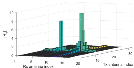
FIGURE 2. Virtual channel matrix without leakage.

FIGURE 3. Virtual channel matrix with leakage.

matrixHis known, the relationship between the virtual chan-nel coefficient matrixHV and the real channel matrix can be written as

HV =VHRHVT, (4)

since VR and VT are DFT matrices and they share

property that VH_R/TVR/T = I, where I is the identity matrix.

It should be noted that HV suffers from leakage from

a specific bin to adjacent bins, which means the number of bins with non-zero values are not L, and the adjacent bins also have relatively large amplitudes. For instance, there is a virtual channel transformed from the real

chan-nel with two chanchan-nel paths (L = 2 in this example) by

using (4). Fig. 2 and 3 compare the difference between the virtual channels with and without leakage. Fig.2 plots the virtual channel with two paths without adjacent leakage. The magnitudes of the two main channel paths are clearly distinct from adjacent bins which have zero or very small magnitudes. However, Fig. 3 illustrates the virtual nel with adjacent leakage. Although the two main chan-nel paths can be seen clearly, the adjacent bins also have non-negligible magnitudes. In other words, the adjacent bins may also contain part of the CSI and should be considered in channel estimation. Consequently, the sparsity of the vir-tual channel is generally more than the number of channel paths.

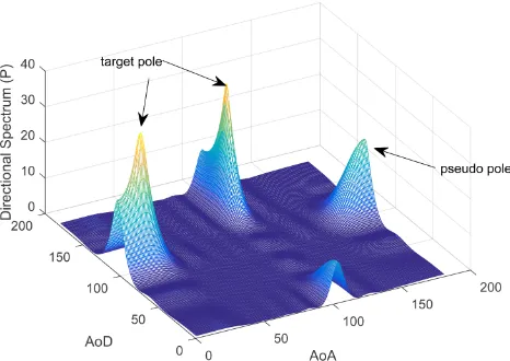
FIGURE 4. Spectrum ambiguity in 2-D MUSIC.

spectrum ambiguity problem mentioned in [10]. As shown in Fig. 4, the spectrum ambiguity problem is that the extreme point of the directional spectrum may be more than the targets we look for. So when searching for the poles of the directional function, the pseudo pole may take the place of the target pole. For the uplink, the UE transmits the pilot signal X∈_CNT×XL_{to the gNB, whereX}

Lis the length of the signal transmitted over each antenna. Then the received signal can be shown as

Y=WH_ABFHUABFX+WHABFZ

=WH_ABFARDαATHUABFX+WHABFZ, (5)

whereUABFandWABFare the analog precoding and combin-ing matrices, respectively. They are obtained from the DFT

codebook. Z is Gaussian white noise with zero mean and

unit variance. Due to the received signal passing through the ABF receiving matrix, the channel information suffers from a certain degree of loss. This dimension-deficient property makes channel estimation in HBF systems more challenging than traditional channel estimation.

III. ALGORITHM DESIGN

Thanks to its wide-ranging applications in sparse signal pro-cessing, compressive sensing is widely used in sparse chan-nel estimation [9], [16], [18], [19]. While CS algorithms may exhibit the floor effect when used in channel estimation [19], the floor effect appears when the channel length is close to or larger than the guard interval (GI). Ding et al.[19] used the prior known pseudo noise (PN) to replace the cyclic prefix (CP) and part of the PN is used to estimate the channel. Consequently, when the channel length (i.e. the maximum channel delay) is close to or larger than the guard interval (the length of the PN), there will be limited PN that can be used to estimate the channel. In other words, the PN during the channel delay time cannot be used for channel estimation, since the PN has been contaminated by the block inter-ferences. So if the channel length is close to or larger than the GI, there will be no more PN left to estimate the channel.

This scenario arises in digital television/terrestrial multime-dia broadcasting (DTMB), which is not common in wireless communication. So, we will only discuss scenarios where the channel length is smaller than the GI.

As can be seen from Fig. 3, mmWave channels are natu-rally sparse, which means CS technology is a nature fit for estimating mmWave channels. The overcomplete dictionary has a major place in CS algorithms. The overcomplete dic-tionary of contrast algorithm in SectionIII-Ais constructed using a universal method, while our proposed algorithm in SectionIII-Bconstructs the dictionary in an adaptive manner. Compared with the contrast algorithm, the proposed adaptive algorithm is slightly more complex, but the system perfor-mance is better, which is shown in SectionIV.

A. CONTRAST ALGORITHM

CS channel estimation needs to first construct an overcom-plete dictionary of the sparse channel. The conventional

overcomplete dictionary2=8Vis composed of a random

measurement matrix8, suh as a Gaussian matrix or a random

±1 matrix, and a basis matrixV[12], [15]. This approach is of low complexity and fast computation.

Based on the approach above, we propose a simple CS algorithm for HBF channel estimation as a contrast. As the arrival and departure steering matrices are unknown, we use virtual channel representation [16], [17]. It follows from the property of Kronecker product that the desired receive signal in (5) can be expressed as

Ydesired =WHABFARDαAHTUABFX

=WH_ABFAR

⊗AH_TUABFX

T

vec(D_α)

=WH_ABFVR

⊗VH_TUABFX

T

hS, (6)

where hS is the vectorization of Dα and a sparse vector containing the elements of the virtual channel matrix HV. Then we vectorize the received signalYas

vec(Y)=GhS+vec WHABFZ

G= WH

ABFVR

⊗ VH TUABFX

T_. (7)

Because matrix G ∈ _CNRFMt×MrXL _{does not satisfy}

the Restricted Isometry Property (RIP), so G cannot be

used as the dictionary for estimating the channel directly.

Baraniuk [12] show that an M ×N i.i.d. Gaussian matrix

can be shown to have the RIP with high probability, if M _> cKlog NKwithcbeing a small constant, whereKis the sparsity of the signal to be estimated. If the Gaussian matrix is multiplied by an orthonormal basis, the product also satisfies the RIP with high probability. So lettingM = NRFNT and

N = NRL, decomposing Gusing SVD, and ignoring the

noise, (7) can be rewritten as

vec(Y)=U1DVH1hS, (8)

whereU1∈ CM,D∈CM×N andV1∈CN. Premultiplying

D†is the pseudo-inverse matrix ofD.VH

1 is an orthonormal

basis, so we premultiply a Gaussian matrix81on the both sides of (8) to obtain

81D†UH₁vec(Y)=81VH₁hS. (9)

Denoting the observation signal byy˜ = 81D†UH

1vec(Y)

and the overcomplete dictionary by21=81VH

1, we have

˜

y1=21hS. (10)

The reconstruction ofh_Sfromy˜can be done via "l0-norm"

minimization, which can be expressed by

ˆ

h_S =arg min hS

kh_Sk_l

0

s.t.y˜1=21hS. (11)

B. ADAPTIVE OVERCOMPLETE DICTIONARY CS

In contrast with the CS algorithm above, we propose an adap-tive overcomplete dictionary for dimension-deficient chan-nel estimation. In order to satisfy the RIP, there is a new way to build the overcomplete dictionary. According to [14], we have the fixed basis matrixV2=VH1. It should be noted

that one can preselect a basis matrixV2different from this

paper. Then matrix82can be designed to satisfy22H22≈I, where22=82V2. We assume that

2H

222=V

H

28

H

282V2≈I. (12)

MultiplyingVH₂ andV2on both sides of (12), we have

V2VH28H282V2VH2 ≈V2VH2. (13)

If V2VH2 has the eigenvalue decomposition V2VH2 =

U23UH₂, then (13) becomes

U23UH₂8H₂82U23UH₂ ≈U23UH₂. (14)

Then letting 0=82U2, where 0 = [τ1,· · · ,τM]T and

τ = [τ1,· · ·τ_N]T, the problem becomes equivalent to optimizing0ˆ

ˆ

0=arg min

3−30

H₀₃

2

F. (15)

Then 82 can be generated from 82ˆ = 0ˆUH₂. Conse-quently, we could obtain the overcomplete dictionary by using22ˆ = ˆ82V2.

Let [λ1,· · ·λ_N] be the eigenvalues of the diagonal matrix3, which are ordered in decreasing order, such that

λ1 > λ2 > ... > λN. Then vi can be expressed as the

elements of diagonal matrix 3 multiplied by the ith row

of0, i.e.,

vi=

λ1τi,1,· · ·, λNτi,N

T

. (16)

DefiningEj=3−

m

P

i=1,i6=j

vivT_i , then (15) can be rewritten

as 3− m X

i=1,i6=j

vivTi −vjvTj

2 F =

Ej−vjv

T j 2

F. (17)

Let matrixEj be eigen-decomposed, i.e.,Ej = Bj6jBT_j ,

where6 = diag(ξ1,· · ·, ξ_M), and B = β1,· · · ,β_MT. Obviously, the objective of the optimization is to minimize the right hand side of (17). So let vj = pξmax,jβmax_,j, whereξmax_,j is the maximum eigenvalue ofEjandβmax_,jis the corresponding eigenvector, and thus the primary gap of Ej−vjvT_j can be eliminated. Thenτj =τj,1,· · ·, τj,N

T is updated as follows

λ1τˆ_j,1,· · · , λ_Nτˆ_j,NT =pξmax_,jβmax_,j. (18)

Then we can obtain the optimal0ˆ usingτj = ˆτj. Further-more, matrix82ˆ and dictionary22are expressed as

ˆ

82=0ˆUH₂

ˆ

22= ˆ82V2. (19)

To construct the newly observed signal according to (19), the original received signal in (8) can be rewritten as

ˆ

0UH₂D†UH₁vec(Y)= ˆ0UH₂V2hS

˜

y2 = ˆ22hS, (20)

wherey˜2 = ˆ0UH2D†UH1vec(Y) and22ˆ = ˆ0UH2V2, which

is calculated inAlgorithm 1,Part I. Through employing the compressive sampling match pursuit (CoSaMP) algorithm for CS reconstruction via (20), we obtain the sparse vectorhS. Thus, the estimated channel can be written as

ˆ

H=VRHˆVVHT, (21)

whereHˆVis the de-vectorization ofhS(inAlgorithm 1,hSis replaced byhˆiK ).

The notation in Part II inAlgorithm 1 is explained as follows.ri is the residual andiis the number of iterations.

i is the set of indexes (i.e., column numbers). 2i is the set of columns from2ˆ, and the columns are selected byi. J0means the set of 2K indexes selected from each iteration.

This is different from orthogonal matching pursuit (OMP). In other words, the traditional OMP algorithm chooses only one maximum value and the corresponding index from each iteration. By contrast, CoSaMP chooses 2Kmaximum values and the corresponding indexes from each iteration. This is an improvement over OMP, which helps reduce the influence of accidental errors such as noise.

To summarize, the proposed algorithm consists of the fol-lowing two steps, which are detailed in Algorithm 1:

(1) Design the overcomplete dictionary2ˆ; (2) Estimate the channel using CoSaMP.

Assuming the number of rows of2ˆ is far less than that of columns, i.e.,M N, the complexity of Algorithm 1 is

O M N3 ≈ O N3 . This complexity is similar to

that in [11].

IV. SIMULATION RESULTS

Algorithm 1 Overcomplete Dictionary Design & CoSaMP-Based Channel Estimation

Require: G,K,M,y˜,AT ,AR

Ensure: Hˆ

1: %Part I— Overcomplete dictionary design

2: Basis matrixV2, a random initial matrix8.

3: Calculate the eigen decompositionV2V2H = U23U2H

;0=8U2.

4: foreachi∈[1,M]do

5: Calculate the eigenvalues ofEj

6: Find the maximum eigenvalue ξmax_,j and the

corre-sponding eigenvectorβmax_,j

7: Update the components ofOτjusing (18)

8: end for

9: Calculate the optimal8=ˆ O0U2H,2ˆ =8ˆV2.

10: %Part II— CE-CoSaMP

11: r0= ˜y,0= ∅,20= ∅. 12: foreachi∈[1,K]do

13: Calculateu= ˆ2Hri−1=

h

ˆ θ1,· · · ˆθ_N

iH ri−1

14: Find the maximum 2K values ofu, and let the corre-sponding column indexesj2K constitute setJ0 15: Leti=i−1∪J0,2i=2i−1∪ ˆθj forall j∈J0

16: Calculatehˆ_i=arg min hi

y˜−2_ih_i

= 2T_i 2_i

−1

2T i y˜

17: Find the maximum K values ofhˆiand let them behˆiK ; the corresponding K columns of2ibe the2iK; the columns indexes of₂ˆ _be

iK

18: Update i = iK, ri = Qy − 2iKhˆiK = Qy −

2iK 2Ti 2i

−1

2T i y˜

19: If ri < 10−15 (which means the residual is small enough).

20: end for

De-vectorize

21: thehˆiK intoHˆV

22: CalculateHˆ =ARHˆVAHT

the number of chainsNRF = 2, . . . ,6. The virtual channel

sparsity is K = L = 6, which means the non-zero value

of HV is 6. We chose the virtual channel without leakage in our simulation, because the sparsity of the virtual channel with leakage is much larger than the number of channel paths (K > L) and usually is not clear. The NMSE is adopted as the performance metric, which is defined as

NMSE=10log₁₀

ˆ

H−H

2

F

kHk2

F

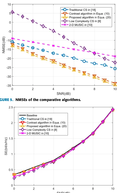
. (22)

Fig. 5 depicts the NMSEs of five comparative channel estimation schemes. The number of RF chains in this sim-ulation case is fixed to 6. The circle, rhombus, star, inverted triangle and triangle lines indicate the performances of the CE algorithm of traditional CS in [18], the 2-D MUSIC algorithm in [10], the low-complexity algorithm in [8], the contrast algorithm based upon (10) and the proposed algorithm based

FIGURE 5. NMSEs of the comparative algorithms.

FIGURE 6. SEs of the comparative algorithms versus the baseline with perfect CSI.

upon (20), respectively. As can be observed from the figure, the algorithm proposed in this paper outstrips the others in the sense of the NMSE. The algorithm in [8] has the worst performance and is almost 15 dB worse than its comparative counterparts at low SNRs. This is because the algorithm in [8] estimates the sparse channel coefficient matrix and the two angle matrices (AOA and AOD) at the same time. The esti-mation errors caused by noise have greater influence than the other algorithms, especially at low SNRs. The 2-D MUSIC and traditional CS algorithms perform very close to the pro-posed two algorithms in this paper at low SNRs, but the gap grows when SNR increases. While 2-D MUSIC is slightly worse than the traditional CS method, because the method to estimate the path gain used in [10] is least-square (LS). In other words, the LS algorithm is sensitive to noise and the estimation results are easily affected by the noise. Further-more, the results demonstrate that the CS algorithm with the adaptive dictionary sees a certain improvement in NMSE over the universal dictionary scheme.

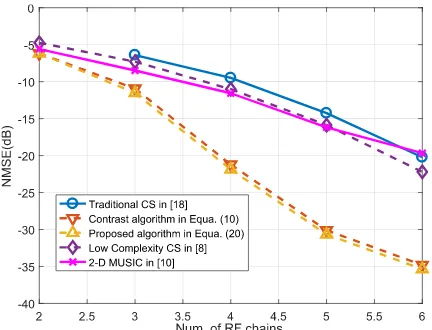
FIGURE 7. NMSEs of the comparative algorithms versus the number of RF chains.

the channel estimation results in [8] are not as good as those of the other methods, which is shown in Fig. 5.

FIGURE 8. SEs of the comparative algorithms versus the number of RF chains.

Fig.7 and 8 show the effects of the number of RF chains on

the NMSE and the SE at SNR=10 dB. We do not consider

the traditional CS algorithm in [18] whenNRF =2, because there are errors in calculatinghˆiwhenNRF = 2. When the number of RF chains is two, the rank of the ABF matrix equals two, i.e.,rank(UT_ABF) =rank(WH_ABF) =2. Then the rank of the sensing matrixrank(8ˆ)=rank(UT_ABF⊗WH_ABF)=

4<K. Consequently, matrix2i(inAlgorithm 1, line 15) is singular matrix when updating it and the calculation ofhˆiwill be wrong because matrix2T_i 2iis not full rank and cannot be inverted. Fig. 7 indicates that the proposed algorithm reaps nearly 30 dB gains in NMSE, when the number of RF chains grows from 2 to 6. While the SE in Fig.8 converges to the upper band after the number of RF chains becomes more than 5. This is because the data streams limit the growth of SE in the network.

V. CONCLUSION

In this paper, we proposed a defective-dimension chan-nel estimation algorithm based on CS technology. Com-pared with non-adaptive algorithms, the proposed algorithm

designed an overcomplete dictionary adaptively with the objective of improving the channel estimation performance in terms of NMSE. The proposed scheme also shows a better noise robustness performance than the existing methods, and the SE is close to the upper bound of perfect CSI. Our future research will focus on two more challenging scenarios. One is CS channel estimation for virtual channels with adjacent leakage, while the other one is when sparsity is nota priori known.

REFERENCES

[1] J. Nightingale, J. M. A. Calero, Q. Wang, and P. Salva-Garcia, ‘‘5G-QoE: QoE modelling for ultra-HD video streaming in 5G networks,’’IEEE Trans. Broadcast., vol. 64, no. 2, pp. 621–634, Jun. 2018.

[2] Z. Pi and F. Khan, ‘‘An introduction to millimeter-wave mobile broadband systems,’’IEEE Commun. Mag., vol. 49, no. 6, pp. 101–107, Jun. 2011. [3] T. S. Rappaportet al., ‘‘Millimeter wave mobile communications for 5G

cellular: It will work!’’IEEE Access, vol. 1, pp. 335–349, 2013. [4] F. Sohrabi and W. Yu, ‘‘Hybrid digital and analog beamforming design for

large-scale antenna arrays,’’IEEE J. Sel. Topics Signal Process., vol. 10, no. 3, pp. 501–513, Apr. 2016.

[5] O. El Ayach, S. Rajagopal, S. Abu-Surra, Z. Pi, and R. W. Heath, Jr., ‘‘Spatially sparse precoding in millimeter wave MIMO systems,’’IEEE Trans. Wireless Commun., vol. 13, no. 3, pp. 1499–1513, Mar. 2014. [6] A. Alkhateeb, G. Leus, and R. W. Heath, Jr., ‘‘Limited feedback hybrid

precoding for multi-user millimeter wave systems,’’IEEE Trans. Wireless Commun., vol. 14, no. 11, pp. 6481–6494, Nov. 2015.

[7] A. Alkhateeb, O. El Ayach, G. Leus, and R. W. Heath, Jr., ‘‘Channel estimation and hybrid precoding for millimeter wave cellular systems,’’

IEEE J. Sel. Topics Signal Process., vol. 8, no. 5, pp. 831–846, Oct. 2014. [8] H.-L. Chiang, T. Kadur, G. Fettweis, and W. Rave, ‘‘Low-complexity spatial channel estimation and hybrid beamforming for millimeter wave links,’’ in Proc. IEEE Int. Symp. Pers., Indoor Mobile Radio Commun. (PIMRC), Valencia, Spain, Sep. 2016, pp. 942–948.

[9] Y. Han and J. Lee, ‘‘Asymmetric channel estimation for multi-user mil-limeter wave communications,’’ inProc. IEEE Int. Conf. Inf. Commun. Technol. Converg. (ICTC), Jeju, South Korea, Oct. 2016, pp. 4–6. [10] Z. Guo, X. Wang, and W. Heng, ‘‘Millimeter-wave channel

estima-tion based on 2-D beamspace MUSIC method,’’IEEE Trans. Wireless Commun., vol. 16, no. 8, pp. 5384–5394, Aug. 2017.

[11] M. L. Bencheikh, Y. Wang, and H. He, ‘‘Polynomial root finding technique for joint DOA DOD estimation in bistatic MIMO radar,’’Signal Process., vol. 90, no. 9, pp. 2723–2730, Mar. 2010.

[12] R. G. Baraniuk, ‘‘Compressive sensing [lecture notes],’’IEEE Signal Process. Mag., vol. 24, no. 4, pp. 118–124, Jul. 2007.

[13] T. E. Bogale, L. B. Le, and X. Wang, ‘‘Hybrid analog-digital channel estimation and beamforming: Training-throughput tradeoff,’’IEEE Trans. Commun., vol. 63, no. 12, pp. 5235–5249, Dec. 2015.

[14] J. M. Duarte-Carvajalino and G. Sapiro, ‘‘Learning to sense sparse signals: Simultaneous sensing matrix and sparsifying dictionary optimization,’’

IEEE Trans. Image Process., vol. 18, no. 7, pp. 1395–1408, Jul. 2009. [15] D. L. Donoho, ‘‘Compressed sensing,’’IEEE Trans. Inf. Theory, vol. 52,

no. 4, pp. 1289–1306, Apr. 2006.

[16] J. Sung, J. Choi, and B. L. Evans. (2017). ‘‘Wideband channel esti-mation for hybrid beamforming millimeter wave communication sys-tems with low-resolution ADCs.’’ [Online]. Available: https://arxiv.org/ abs/1710.10669

[17] A. M. Sayeed, ‘‘Deconstructing multi-antenna fading channels,’’IEEE Trans. Signal Process., vol. 50, no. 10, pp. 2563–2579, Oct. 2002. [18] W. U. Bajwa, J. Haupt, A. M. Sayeed, and R. Nowak, ‘‘Compressed

channel sensing: A new approach to estimating sparse multipath channels,’’

Proc. IEEE, vol. 98, no. 6, pp. 1058–1076, Jun. 2010.

[19] W. Ding, F. Yang, C. Pan, L. Dai, and J. Song, ‘‘Compressive sensing based channel estimation for OFDM systems under long delay channels,’’IEEE Trans. Broadcast., vol. 60, no. 2, pp. 313–321, Jun. 2014.

[20] A. F. Molischet al., ‘‘Hybrid beamforming for massive MIMO: A survey,’’

IEEE Commun. Mag., vol. 55, no. 9, pp. 134–141, Sep. 2017.

YU XIAO received the B.S. degree from Xidian University, Xi’an, China, in 2011, and the M.S. degree from the North China University of Tech-nology, Beijing, China, in 2016. He is currently pursuing the Ph.D. degree with the Key Labora-tory of Universal Wireless Communications, Min-istry of Education, Beijing University of Posts and Telecommunications, China. His research interests include hybrid beamforming, channel estimation, and compressive sensing.

YAFENG WANG (S’00–M’03–SM’09) received the B.Sc. degree from the Baoji University of Arts and Science, in 1997, the M.Eng. degree from the University of Electronic Science and Tech-nology of China, in 2000, and the Ph.D. degree from the Beijing University of Posts and Telecom-munications, in 2003. In 2008, he was a Visit-ing Scholar with the Faculty of EngineerVisit-ing and Surveying, University of Southern Queensland, Australia.

He is currently a Professor of electronic engineering with the School of Information and Telecommunications, Beijing University of Posts and Telecommunications. He leads the Broadband Mobile Communication Engi-neering Laboratory, which is one of the Zhongguancun Science Park Open Laboratories. He has authored or co-authored over 100 peer-reviewed journal and conference papers. His research mainly focuses on wireless communi-cations and information theory.

WEI XIANG (S’00–M’04–SM’10) received the B.Eng. and M.Eng. degrees in electronic engi-neering from the University of Electronic Sci-ence and Technology of China, Chengdu, China, in 1997 and 2000, respectively, and the Ph.D. degree in telecommunications engineering from the University of South Australia, Adelaide, Australia, in 2004. From 2004 to 2015, he was with the School of Mechanical and Electrical Engineering, University of Southern Queensland, Toowoomba, Australia. He is currently the Founding Professor and the Head of the Discipline of the Internet of Things Engineering with the College of Science and Engineering, James Cook University, Cairns, Australia. He has authored or co-authored over 200 peer-reviewed journal and conference papers. His research interests include the broad areas of communications and information theory, particularly the Internet of Things, and coding and signal processing for multimedia communications systems. He is an Elected Fellow of the IET and the Engineers Australia. He was named as a Queensland Inter-national Fellow by the Queensland Government of Australia, from 2010 to 2011, as an Endeavour Research Fellow by the Commonwealth Government of Australia, from 2012 to 2013, as a Smart Futures Fellow by the Queensland Government of Australia, from 2012 to 2015, and as a JSPS Invitational Fellow jointly by the Australian Academy of Science and the Japanese Society for Promotion of Science, from 2014 to 2015. He was a Finalist of the 2016 Pearcey Queensland Award. He was a recipient of the TNQ Innovation Award, in 2016. He was a co-recipient of three best paper awards at 2015 WCSP, 2011 IEEE WCNC, and 2009 ICWMC. He received several prestigious fellowship titles. He is the Vice Chair of the IEEE Northern Australia Section. He was an Editor ofIEEE COMMUNICATIONS LETTERS, from

2015 to 2017. He is an Associate Editor ofTelecommunications Systems