Nonlinear Physics in Soliton Microcombs

(1)

Thesis by

Qifan Yang

In Partial Fulfillment of the Requirements for the Degree of

Doctor of Philosophy

CALIFORNIA INSTITUTE OF TECHNOLOGY

Pasadena, California

2019

(2)

Qifan Yang

ORCID: 0000-0002-7036-1712

(3)

ACKNOWLEDGEMENTS

First and foremost, I am deeply grateful to my advisor, Prof. Kerry Vahala, for his

support and guidance over the years. More than an distinguished scientist, Prof.

Vahala is no doubt the best mentor that I can ever imagine. He has given me complete

freedom to exploit my research interest with valuable instructions. His devotion in science has motivated me to always stay hungry and stay foolish. Prof. Vahala is

the perfect example as a scientist and mentor that I wish to follow throughout my

career. It is a pride and a privilege to have ever been his student.

I would like to express my gratitude to Prof. Oskar Painter, Prof. Paul Bellan, and

Prof. Andrei Faraon for their service as my graduation committee and insightful

input to my thesis. I would also like to thank Dr. Scott Diddams, Prof. Tobias

Kippenberg, Prof. Lan Yang, Prof. John Bowers, Prof. Amnon Yariv, and Prof. Qiang Lin for their support of my research and academic career.

My heartfelt appreciation goes to my colleagues. I would like to offer my special

thanks to Dr. Xu Yi, Dr. Ki Youl Yang and Dr. Myoung-Gyun Suh for their

helpful advice as well as productive collaborations. I gratefully acknowledge Dr.

Seunghoon Lee, Dr. Dongyoon Oh, Dr Hansuek Lee, Dr. Yu-Hung Lai, Dr. Xinbai

Li and Dr. Chengying Bao for their support. I also want to thank Boqiang Shen,

Heming Wang, Xueyue Zhang, Lue Wu, and Zhiquan Yuan for their fidelity in

research. I likewise thank Zhewei Zhang, Yonghwi Kim, Wen Hui Cheng, and Wei-Siang Lin in Caltech, Junqiu Liu from EPFL, and Dr. Minh Tran and Dr. Nicolas

Volet from UCSB, as well as Yang He from Rochester for the exciting collaborations.

Special thanks also to my former advisor, Prof. Yun-Feng Xiao, for his

hand-by-hand training and continuous support. I was fortunate to start my research under his

guidance.

Finally, I owe my deepest gratitude to my family for their continuous and unparalleled love, help, and support. They sparked my curiosity for the world in my childhood,

without which I would have never been a scientist by now. I am also deeply thankful

to my wife, Yi Xin, for the resonance between us which has infinite Q factor. The

journey we have survived has been an invaluable and unforgettable experience. With

(4)

ABSTRACT

Like rulers of light, optical frequency combs consist of hundreds to millions of

coherent laser lines, which are capable of measuring time and frequency with the

highest degree of accuracy. Used to rely on table-top mode-locked lasers, optical

frequency combs have been recently realized in a miniaturized form, namely the microcomb, using monolithic microresonators. Besides a reduction of footprint,

microcombs could also achieve parity with traditional frequency combs in

perfor-mance by mode-locking through the formation of “light bullets” called dissipative

Kerr solitons. These soliton microcombs not only serve as a unique platform to

study nonlinear physics, but also offer scalable and cost-effective solutions to many

groundbreaking applications, spanning spectroscopy to time standards. In this thesis

I will trace the physical origin of soliton microcombs, followed by their experimental

realization in high-Q silica microresonators. The impact of several nonlinear

pro-cess on solitons will be discussed, which leads to novel soliton systems, e.g., Stokes solitons and counter-propagating solitons. Utilizing these nonlinear properties, we

show that soliton microcombs can be adapted for high-precision spectroscopic

appli-cations. In the end, a real-time method for monitoring transient behavior of solitons

(5)

PUBLISHED CONTENT AND CONTRIBUTIONS

[1] Yang He*, Qi-Fan Yang*, Jingwei Ling, Rui Luo, Hanxiao Liang, Mingxiao Li, Boqiang Shen, Heming Wang, Kerry Vahala, and Qiang Lin. A self-starting bi-chromatic LiNbO3 soliton microcomb. arXiv preprint arXiv:1812.09610, 2018. URL: https://arxiv.org/abs/1812.09610

Q.-F.Y conducted the experiment, prepared the data, and participated in the writing of the manuscript.

[2] Seung Hoon Lee*, Dong Yoon Oh*, Qi-Fan Yang*, Boqiang Shen*, Heming Wang*, Ki Youl Yang, Yu-Hung Lai, Xu Yi, Xinbai Li, and Kerry Vahala. Towards visible soliton microcomb generation.Nat. Commun., 8(1295), 2017. DOI: 10.1038/s41467-017-01473-9

Q.-F.Y participated in the conception of the project, conducted the experiment, prepared the data, and participated in the writing of the manuscript.

[3] Xinbai Li*, Boqiang Shen*, Heming Wang*, Ki Youl Yang*, Xu Yi, Qi-Fan Yang, Zhiping Zhou, and Kerry Vahala. Universal isocontours for dissipative kerr solitons. Opt. Lett., 43(11):2567–2570, 2018. DOI: 10.1364/OL.43.002567

Q.-F.Y participated in the experiment.

[4] Myoung-Gyun Suh*, Qi-Fan Yang*, and Kerry J Vahala. Phonon-limited-linewidth of brillouin lasers at cryogenic temperatures. Phys. Rev. Lett., 119(14):143901, 2017. DOI: 10.1103/PhysRevLett.119.143901

[5] Myoung-Gyun Suh*, Qi-Fan Yang*, Ki Youl Yang, Xu Yi, and Kerry J Vahala. Microresonator soliton dual-comb spectroscopy.Science, 354(6312):600–603, 2016. DOI: 10.1126/science.aah651

[6] Nicolas Volet, Xu Yi, Qi-Fan Yang, Eric J Stanton, Paul A Morton, Ki Youl Yang, Kerry J Vahala, and John E Bowers. Micro-resonator soliton generated directly with a diode laser. Laser Photonics Rev., 12(5):1700307, 2018. DOI: 10.1002/lpor.201700307

Q.-F.Y participated in the experiment.

(6)

Q.-F.Y participated in the experiment, prepared the data, and participated in the writing of the manuscript.

[8] Qi-Fan Yang*, Boqiang Shen*, Heming Wang*, Minh Tran, Zhewei Zhang, Ki Youl Yang, Lue Wu, Chengying Bao, John Bowers, Amnon Yariv, et al. Vernier spectrometer using counterpropagating soliton microcombs. Science, 363(6430):965–968, 2019. DOI: 10.1126/science.aaw2317

Q.-F.Y conceived the project, conducted the experiment, prepared the data, and participated in the writing of the manuscript.

[9] Qi-Fan Yang*, Xu Yi*, Ki Youl Yang, and Kerry Vahala. Spatial-mode-interaction-induced dispersive waves and their active tuning in microres-onators. Optica, 3(10):1132–1135, 2016. DOI: 10.1364/OPTICA.3.001132 Q.-F.Y participated in the conception of the project, conducted the experiment, prepared the data, and participated in the writing of the manuscript.

[10] Qi-Fan Yang*, Xu Yi*, Ki Youl Yang, and Kerry Vahala. Stokes solitons in optical microcavities.Nat. Phys., 13(1):53–57, 2017. DOI: 10.1038/nphys3875 Q.-F.Y participated in the conception of the project, conducted the experiment, prepared the data, and participated in the writing of the manuscript.

[11] Qi-Fan Yang*, Xu Yi*, Kiyoul Yang, and Kerry Vahala. Counter-propagating solitons in microresonators. Nat. Photon., 11(9):560–564, 2017. DOI: 10.1038/nphoton.2017.117

[12] Xu Yi*, Qi-Fan Yang*, Ki Youl Yang*, Myoung-Gyun Suh, and Kerry Vahala. Soliton frequency comb at microwave rates in a high-Q silica microresonator. Optica, 2(12):1078–1085, 2015. DOI: 10.1364/OPTICA.2.001078

[13] Xu Yi*, Qi-Fan Yang*, Ki Youl Yang, and Kerry Vahala. Active capture and stabilization of temporal solitons in microresonators. Opt. Lett., 41(9):2037– 2040, 2016. DOI: 10.1364/OL.41.002037

[14] Xu Yi*, Qi-Fan Yang*, Ki Youl Yang, and Kerry Vahala. Theory and measure-ment of the soliton self-frequency shift and efficiency in optical microcavities. Opt. Lett., 41(15):3419–3422, 2016. DOI: 10.1364/OL.41.00341

(7)

[16] Xu Yi*, Qi-Fan Yang*, Xueyue Zhang*, Ki Youl Yang, Xinbai Li, and Kerry Vahala. Single-mode dispersive waves and soliton microcomb dynamics.Nat. Commun., 8:14869, 2017. DOI: 10.1038/ncomms14869

(8)

LIST OF ILLUSTRATIONS

Number Page

1.1 Time and frequency domain representation of an optical frequency

comb. (a) A periodic pulse train with periodT (repetition rate fr).

The carrier wave (red) and envelope (grey) are propagating at phase

velocity and group velocity, respectively, which causes an increasing

carrier-envelope phase offset (∆φo) between consecutive pulses. (b)

The optical spectrum of an OFC. The comb teeth (red) are separated

by fr, while the offset frequency is related to the carrier-envelope phase offset by fo = fr∆φo/2π. The frequency of the comb tooth of orderncan be expressed as fn= fo+n fr. A common method to

deter-mine the offset frequency is called frequency comb self referencing.

Specifically, the low-frequency portion of the OFC is

frequency-doubled and mixed with its high-frequency portion, which gives the

offset frequency fo. (c) The optical spectrum of a fiber mode-locked

laser. The repetition rate is 250 MHz, and the comb teeth are not

resolved by the optical spectral analyzer. The inset shows a fiber

mode-locked laser. . . 3 1.2 Multiple types of microresonators. (a) A Fabry-P´erot-type

microres-onator. (b) A whispegallery-mode microresmicrores-onator. (c) A

ring-shaped microresonator. (d) A silica whispering-galley-mode

mi-croresonator on a chip. The photo is provided in courtesy of Lue

Wu. . . 6

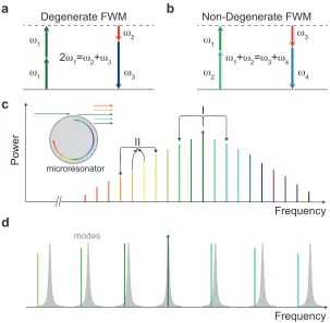
1.3 Principle of microcomb generation. (a)-(b) Level diagrams showing

degenerate and non-degenerate FWM process. (c) The optical

spec-trum of a microcomb, where the central arrow represents the pump.

Process I (II) corresponds to the degenerate (non-degenerate) FWM process. (d) Schematic representation of comb teeth and resonant

modes. When moving away from the pump, the increasing offset

between the comb tooth and the modes is induced by group velocity

(11)

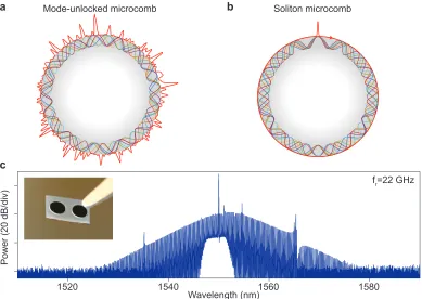
1.4 Soliton microcombs. (a)-(b) Schematic illustrations showing a

mode-unlocked comb and a soliton comb. The oscillations in the resonator represent spectral components of the comb, while the exterior red

lines indicate the intracavity power. (c) A typical spectrum of a

soliton microcomb. The repetition rate is 22 GHz. Inset: silica

microresonators. . . 8

2.1 Schematic illustration of a continuously-driven microresonator. (a)

Coordinates of lab frame. (b) Coordinates of rotational frame. . . 17

2.2 Numerical simulation of LLE. (a) Total intracavity power versus

de-tuning while the pump is tuned across a resonance with increasing

detuning. Parameters used in simulation: f = 50;D2/κ= 0.01. 512 modes are involved. (b) Intracavity intensity versus polar angle at

dif-ferent detunings as marked in (a). I: Turing pattern; II: modulational

instability comb; III: solitons. . . 26

3.1 Silica wedge resonator. (a) Top view of a silica wedge resonator

taken by scanning electron microscope (SEM). The scale bar is 1

mm. Image is from Lue Wu. (b) SEM image showing cross section

of a wedge resonator. The scale bar is 5 µm. Image is from Dr.

Seung Hoon Lee. (c) Finite element method (FEM) simulation of

TM1 mode profile. (d) Typical transmission spectrum while tuning a laser across a high-Q mode in a wedge resonator with 3 mm in

diameter and 8 µm in thickness. The Lorentzian fitting (red) reveals

intrinsic Q factor over 300 million. . . 28

3.2 Dispersion engineering via resonator thickness control. (a) A

ren-dering of a silica resonator with the calculated mode profile of the

TM1 mode superimposed. (b) Cross-sectional SEM images of the

fabricated resonators with different thickness. White scale bar is 5

µm. (c) Simulated regions of normal and anomalous dispersion are shown versus silica resonator thickness (t) and pump wavelength. The zero dispersion wavelength (λZ DW) for the TM1 mode appears

as a blue curve. Plot is made for a 3.2-mm-diameter silica resonator.

Three different device types, I, II, and III, which correspond to top,

mid, and bottom panels in (b), are indicated for soliton generation at

1550 nm, 1064 nm, and 778 nm. The simulation is performed by Dr.

(12)

3.3 Measured frequency dispersion (blue points) belonging to the

soliton-forming mode families are plotted versus relative mode number, µ. To construct this plot, mode frequency relative to a µ = 0 mode

(mode to be pumped) is measured using a calibrated Mach-Zehnder

interferometer (fiber optic based). To second order in the mode

number, the mode frequency is given by the Taylor expansionωµ = ω0+ µD1+ 1₂µ2D2 and the dashed red curves are parabolic fittings with fitted parameters on the top of each panel. In the plot, the mode

frequencies are offset by the linear term in the Taylor expansion to

make clear the second-order group dispersion. The measured modes

span wavelengths from 1520 nm to 1580 nm and µ= 0 corresponds to a wavelength close to 1550 nm. . . 30

3.4 Pump power transmission versus tuning across a resonance used to

generate the solitons. The data show the formation of steps as the

pump tunes red relative to the resonance. Both blue-detuned and

red-detuned operation of the pump relative to the resonance are inferred

from generation of an error signal using a Pound-Drever-Hall system

operated open loop. . . 32

3.5 (a) Simulated intracavity power in which the pump laser scans over

the resonance from the blue side to the red side. The steps on the red-detuned side indicate soliton formation. (b) Schematic of

experimental setup. (c) Four phases of feedback-controlled soliton

excitation: (I) pump laser scans into cavity resonance from

blue-detuned side; (II) laser scan stops and pump power is reduced (∼

10 µs) to trigger solitons, and then increased (∼ 100 µs) to extend soliton existence range; (III) servo-control is engaged to actively lock

the soliton power by feedback control of laser frequency; (IV) lock

sustains and solitons are fully stabilized. The cavity-pump detuning

(13)

3.6 Demonstration of capture and locking of a soliton state. (a)

Soli-ton excitation with "power kicking" but no active locking is shown. The soliton state destabilizes around 22ms due to thermal transients.

Soliton power is shown in red and a Mach Zehnder (MZI) reference

is in blue. (b) Soliton excitation with active locking is shown with

conditions similar to panel (a). (c) Zoom-in view of panel (b). The

four phases are indicated using the same background color scheme

as in Figure 3.5. . . 35

3.7 Continuous soliton measurement over 19 hours. Soliton power are

plotted versus time in hours. The soliton power experiences a slow

drift to lower values which is attributed to a slow variation in either the power set point of the electronic control or in the detected power

(perhaps due to temperature drift). . . 36

3.8 Experiment setup, soliton mode-family dispersion, optical spectrum

and autocorrelation. (a) Experimental setup. EDFA:

erbium-doped-fiber-amplifier; AOM: acousto-optic modulator; PD: photodetector;

ESA: electrical spectral analyzer; OSA: optical spectral analyzer;

FROG: frequency resolved optical gatings. (b) Measured mode

fam-ily dispersion (blue points) belonging to the soliton-forming mode

family is plotted versus relative mode number, µ. The presence of non-soliton forming mode families can be seen through the

appear-ance of avoided mode crossings (spur-like features) that perturb the

parabolic shape. Simulations of the non soliton mode families

be-lieved to be responsible for these spurs are provided (see mode 1

and mode 2 dashed curves). In addition, the normalized transverse

intensity profiles for the soliton and non-soliton spatial modes are

provided at the top of the panel (red indicates higher mode intensity).

The simulation used the Sellmeier equation for the refractive index of

silica. Oxide thickness, wedge angle, and radius were fine-adjusted to produce the indicated fits. (c) Optical spectrum of single soliton state

is shown with a sech2 envelope (red dashed line) superimposed for

comparison. The pump laser is suppressed by 20 dB with an optical

Bragg filter. (d) FROG (upper) and autocorrelation trace (lower) of

the soliton state inc. The optical pulse period is 46 ps and the fitted

(14)

3.9 Detected phase noise and electrical spectra for three devices with

cor-responding mode dispersion and soliton data. Phase noise spectral density function plotted versus offset frequency from the detected

soliton repetition frequency of three different devices. A Rohde

Schwarz phase noise analyzer was used in the measurement.

In-set shows the electrical spectrum of the soliton repetition frequency

(21.92 GHz) for one device. The other devices had similar

spec-tra with repetition frequencies of 22.01 and 21.92 GHz. The phase

noise of the fiber pump laser is shown in green and was generated

by mixing 2 nominally identical pump lasers to create a 2.7 GHz

electrical beatnote. Several features in the pump laser phase noise are reproduced in the soliton phase noise (see features near and above

20 kHz). The black line connecting square dots is the measurement

floor of the phase noise analyzer. . . 38

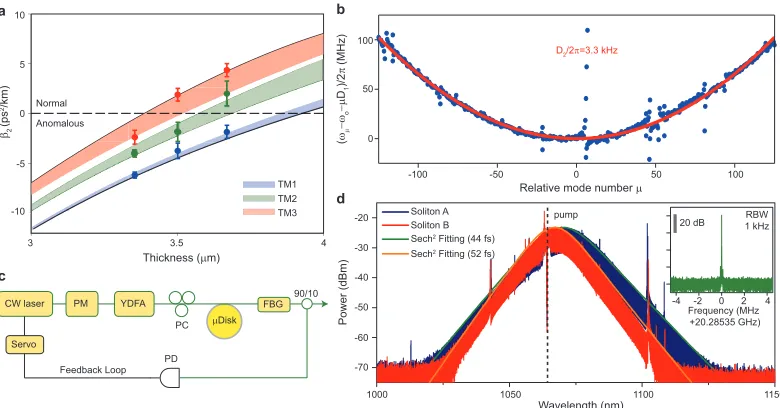
3.10 Microresonator dispersion engineering and soliton generation at 1064

nm. (a) Simulated dispersion (GVD) of TM mode families versus

resonator thickness. The angle of the wedge ranges from 30◦ to

40◦ in the colored regions. Measured data points are indicated and

agree well with the simulation. (b) Measured relative mode

frequen-cies (blue points) plotted versus relative mode number of a soliton-forming TM1 mode family in a 3.4 µm thick resonator. The red

curve is a parabolic fit yielding D2/2π=3.3 kHz. (c) Experimental

setup for soliton generation. A continuous-wave (CW) fiber laser is

modulated by an electro-optic phase modulator (PM) before coupling

to a ytterbium-doped-fiber-amplifier (YDFA). The pump light is then

coupled to the resonator using a tapered fiber. Part of the comb power

is used to servo-lock the pump laser frequency. FBG: fiber Bragg

grating. PD: photodetector. PC: polarization controller. (d) Optical

spectra of solitons at 1064 nm generated from the mode family shown in b. The two soliton spectra correspond to different power levels

with the blue spectrum being a higher power and wider bandwidth

soliton. The dashed vertical line shows the location of the pump

frequency. The solid curves are sech2fittings. Inset: typical detected

electrical beatnote showing soliton repetition rate. RBW: resolution

(15)

3.11 Control of soliton properties. (a) Measured soliton comb output

power is plotted versus measured soliton pulse width (red points) with comparison to Eq. (3.1) (dashed red line). The measured

power per central comb tooth is plotted versus pulse width (blue

points) with comparison to Eq. (3.4) (dashed blue line). (b) The

observed soliton spectra at the limits of the measurement in Figure

3.8(a) is shown (see arrows A and B in Figure 3.8(a)). Solid orange

and green curves are simulations using the Lugiato Lefever equation

including Raman terms. The indicated wavelength shifts between

the pump and the center of the soliton spectrum result from Raman

interactions with the soliton. The location of the pump line for both spectra is indicated by the dashed black line and has been suppressed

by filtering. The inset shows a magnified view near the central

region of the blue spectrum. The green (purple) envelope provides

the Lugiato Lefever simulation with (without) Raman terms. The

green spike is the location of the pump. (c) Measured minimum

pump power for soliton existence is plotted versus measured soliton

pulse width (red points) with comparison to Eq. (3.5) (dashed red

line). Measured efficiency is plotted versus measured soliton pulse

width (blue points) with comparison to Eq. (3.6) (dashed blue line). Simulation using Lugiato-Lefever equation including Raman terms

improves agreement with data (small dashed red and blue lines). . . . 42

4.1 (a) Optical spectra measured for a dissipative Kerr cavity soliton at

two operating points. The pump power is suppressed using a fiber

grating filter. A sech2 fit is shown as the orange curves and pulse

widths inferred from the fitting are shown in the legend. The location

of the pump line is indicated as the black line. The centers of the

spectra are indicated by the green lines. (b) The measured Raman

(16)

4.2 The measured efficiency versus soliton pulse width is plotted (blue

points) for two devices and compared with theory. Theory compar-ison with Raman (solid blue lines) and without Raman (dash blue

lines) is presented. There are no free parameters in the

compari-son. The small deviations between the measurement and the theory

could result from the presence of weak avoided mode crossings in

the dispersion spectrum. . . 53

5.1 Principle of Stokes soliton generation. The Stokes soliton (red)

max-imizes Raman gain by overlapping in time and space with the primary

soliton (blue). It is also trapped by the Kerr-induced effective optical

well created by the primary soliton. . . 56 5.2 Stokes soliton formation in a microresonator. (a) Simulated

intracav-ity comb power during a laser scan over the primary soliton pumping

resonance from the blue (left) to the red (right) of the resonance. The

detuning is normalized to the resonance linewidth. The initial step

corresponds to the primary soliton formation, and the subsequent

decrease in power corresponds to the onset of the Stokes soliton. The

Stokes soliton power is shown in red. (b) Zoomed-in view of the

indi-cated region from panel a. (c) Experimentally measured primary and

Stokes soliton power during a laser scan showing the features simu-lated in panels a and b. (d) Simulation of the intracavity field in the

moving frame of the solitons plotted versus the pump laser detuning.

The detuning axis is scaled identically to Figure panel a. The Figure

shows the primary soliton step region (below threshold) as well as the

onset of the Stokes soliton (above threshold). (e) Temporal overlap of

the primary and Stokes solitons is numerically confirmed in the plot

of normalized power versus location angle within the resonator. The

overlap confirms trapping and co-propagation. (f) Intracavity optical

(17)

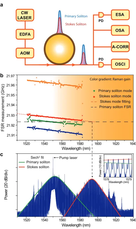
5.3 Experimental setup and observation of Stokes soliton. (a)

Experi-mental setup. (b) Free spectral range (FSR) versus wavelength mea-sured for four mode families in a 3mm disk resonator. The mode

families for the primary and Stokes soliton are shown in green and

red, respectively. The FSR at the spectral center of the primary

soli-ton is shown as a dashed horizontal line. Extrapolation of the Stokes

soliton data (red) to longer wavelengths gives the FSR matching

wave-length where the Stokes soliton forms. The background coloration

gives the approximate wavelength range of the Raman gain spectrum.

(c) Measured primary and Stokes soliton spectra. The Stokes soliton

spectral center closely matches the prediction in (c). Sech2envelopes are shown on each spectrum. The primary soliton spectrum features

a small Raman self-frequency shift. . . 64

5.4 Observation of Stokes solitons in multiple devices. (a) Dispersion

spectra (see Figure 5.3(c)) for the Stokes soliton forming mode

fam-ily measured in three devices (the upper spectrum is the device from

Figure 5.3). Other mode families have been omitted in the plots for

clarity. The horizontal dashed lines give the repetition frequency

of the primary soliton in each device. Extrapolation of the

disper-sion data attained by simulation is provided to graphically locate the predicted Stokes soliton wavelength. (b) The measured primary

and Stokes soliton spectra corresponding to the devices in (a). The

spectral locations of the Stokes solitons agree well with the graphical

predictions. . . 65

5.5 Soliton pulse and frequency measurements. (a)

Frequency-resolved-optical-gating (FROG) traces of the primary and Stokes solitons. The

primary soliton is amplified to 500 mW by an EDFA before coupling

into the FROG setup, while the Stokes soliton is amplified to 10 mW

by two cascaded semiconductor optical amplifiers with gain centered around 1620 nm. The period of the primary and Stokes solitons

are 46 ps, the cavity round trip time. (b) Electrical spectra of the

detected primary soliton pulse stream (blue) and the Stokes pulse

stream (red). (c) Beatnote between neighboring comb teeth of the

primary and Stokes solitons for a device like that in Figure 5.3. The

(18)

5.6 Stokes soliton spectra, power and threshold measurements. (a)

Soli-ton spectra are plotted below and above threshold. The upper in-sets show the spatial mode families associated with the primary and

Stokes solitons. (b) Measurement of Stokes soliton power and

pri-mary soliton peak power versus total soliton power. The pripri-mary

soliton peak power (blue) versus total power experiences threshold

clamping at the onset of Stokes soliton oscillation. The theoretical

threshold peak power from Eq. (5.13) is also shown for comparison

as the horizontal blue dashed line. . . 68

6.1 Dispersive wave generation by spatial mode interaction. (a)

Mea-sured relative-mode-frequencies (blue points) of the soliton-forming mode family and the interaction mode family. Mode number µ = 0

corresponds to the pump laser frequency of 193.45 THz (1549.7

nm). Hybrid mode frequencies calculated from Eq. (6.1) are shown

in green and the unperturbed mode families are shown in orange.

The dashed, horizontal black line determines phase matching for

ωr = D1A. (b) Measured soliton optical spectrum with dispersive wave feature is shown. For comparison, a Sech2 fitting is provided

in red. The pump frequency (black) and soliton center frequency

(green) indicate a Raman-induced soliton self-frequency shift (also see Figure 6.2(c)). A microwave beatnote of the photo-detected

soli-ton and dispersive wave is shown in the inset (frequency scale is offset

(19)

6.2 Dispersive wave phase matching condition and Raman-induced

fre-quency shift. (a) Soliton and interaction mode family dispersion curves are shown (see Figure 6.1(a)) with phase matching dashed

lines (see Eq. (6.4)). The black line is the case whereωr = D1Aand

the green line includes a Raman-induced change inωr. The

intersec-tion of the soliton branch with these lines is the dispersive wave phase

matching point (arrows). (b) Soliton optical spectra corresponding

to small (red) and large (blue) cavity-laser detuning (δω). Sech2

fitting of the spectral envelope is shown as the orange curves. (c)

Left: soliton self-frequency-shift,Ω, versus 1/τ_s4(τsis pulse width). The theoretical line is calculated with Q = 166 million (measured) and Raman shock time 2.7 fs. Right: dispersive wave spectra with

cavity-laser detuning (soliton power and bandwidth) increasing from

lower to upper trace. (d) Measured dispersive-wave peak frequencies

(red points) and soliton repetition rate (blue points) are plotted versus

soliton self-frequency shift. The dashed blue line is a plot of Eq.

(6.3). The dashed red line uses Eq. (6.4) to determine the dispersive

wave frequency (≈ µ_DWD1A+ω0) as described in the text. The offset for the repetition rate vertical scale is D1A =21.9733 GHz. . . 75

7.1 observation of single mode dispersive wave. (a) Measured relative mode frequencies are shown as blue points. The green and yellow

dashed lines represent the fitted relative mode frequencies (∆ωµA

and ∆ωµB) of the unperturbed soliton-forming mode family A and crossing mode family B, respectively. Relative mode frequencies for

upper and lower branch hybrid-modes are∆ω_µ₊ and∆ω_µ−. The red line illustrates the frequencies of a hypothetical soliton frequency

comb. A non-zero slope on this line arises from the repetition rate

change relative to the FSR at mode µ = 0. (b) Measured optical

spectra at soliton operating points I and II, corresponding to closely matched cavity-pump detuning frequencies, δω. A strong

single-mode dispersive wave at µ = 72 is observed for operating point II

and causes a soliton recoil frequency shift. This frequency shift adds

(20)

7.2 Soliton hysteretic behavior induced by mode interaction. (a-b)

Dispersive-wave power and soliton spectral center frequency shift versus cavity-pump detuning. Inset in (a): Measured (blue dots) and theoretical

(red line) recoil frequency versus the dispersive wave power. . . 81

7.3 Numerical simulation and analytical model of single-mode dispersive

wave generation and recoil. (a) Numerical (blue dots) and analytical

(red solid line) soliton total frequency shift versus cavity-pump

de-tuning. Points i, ii, iii, and iv correspond to specific soliton operating

points noted in other Figure panels. (b) Numerical (blue dots) and

analytical (red solid line) dispersive wave power (normalized to total

soliton power) versus cavity-pump detuning. Inset: recoil frequency versus the dispersive wave power. (c) Comb spectra contributions

from the two mode families (blue: soliton forming mode family A;

red: crossing mode family B). (d) Time domain intracavity power.

TRis the cavity round trip time. . . 90

7.4 Soliton repetition frequency and phase noise measurement. (a)

Mea-sured (blue dots) and theoretical (red) soliton repetition frequency

versus pump-cavity detuning. The offset frequency is 22.0167 GHz.

The distinct soliton operating points I, II and III refer to phase noise

measurements in panel b. Point III is near the quiet operation point. (b) Phase noise spectra of detected soliton pulse stream at three

oper-ating points shown in panel a. The black line connecting the square

dots is the measurement floor of the phase noise analyzer. (c) Phase

noise of soliton repetition rates at 25 kHz offset frequency plotted

versus the cavity-pump detuning. The blue and red dots (lines)

de-note the experimental (theoretical) phase noise of the upper (blue)

(21)

7.5 Experimental setup and details on detuning-noise measurement. (a)

The experimental setup includes both the soliton generation and char-acterization setup and a Pound-Drever-Hall (PDH) system operated

open loop. The PDH is added to make possible the pump-cavity

detuning noise measurement. Components included in the set up are

an EOM: electro-optic modulator; EDFA: Erbium-doped fiber

am-plifier; AOM: acousto-optic modulator; PC: polarization controller;

FBG: fiber Bragg grating; PD: photodetector; OSA: optical spectral

analyzer; PNA: phase noise analyzer; LO: local oscillator. The OSA

and and PNA are shown for completeness. They are used to measure

the soliton spectrum and repetition rate phase noise. They are not involved in measuring the detuning frequency noise. (b)

Measure-ments that illustrate the pump-cavity detuning measurement. The

green trace is the measured power transmission when scanning the

pump laser frequency across a cavity resonance. The pump laser is

phase modulated, the transmitted signal is detected and the resulting

photocurrent is then mixed with the PDH local oscillator signal to

gen-erate the PDH error signal. Upon laser scan the PDH error signal (as

measured on the oscilloscope) is generated as shown in the red trace.

The pump laser is filtered using the fiber Bragg grating. The monitor-ing point for the detunmonitor-ing frequency measurement is indicated by the

black dot. In order to convert scanning time into laser frequency, a

calibrated Mach-Zehnder interferometer (MZI) records power

trans-mission (blue trace) on an oscilloscope. The free-spectral-range of

the MZI is 40 MHz. . . 93

7.6 Existence study for the quiet point. The maximum ratios of|∂Ω_Recoil/∂δω|

to |∂Ω_Raman/∂δω|at varying normalized modal coupling rateGand normalized crossing-mode damping rate κB (dashed curve is unity

ratio). The quiet point exists when this ratio is greater than unity (red region). Parameters correspond to a silica resonator. . . 96

7.7 Contour plot of detuning range. Color plot of detuning range of

bistability versus spatial-mode coupling strength,G, and dissipation

rate of crossing mode, κB. All quantities are normalized to the

(22)

8.1 Microresonator-based dual-comb spectroscopy. Two soliton pulse

trains with slightly different repetition rates are generated by contin-uous optical pumping of two microresonators. The pulse trains are

combined in a fiber bidirectional coupler to produce a signal output

path that passes through a test sample as well as a reference output

path. The output of each path is detected to generate an electrical

interferogram of the two soliton pulse trains. The interferogram is

Fourier transformed to produce comb-like electrical spectra having

spectral lines spaced by the repetition rate difference of the soliton

pulse trains. The absorption features of the test sample can be

ex-tracted from this spectrum by normalizing the signal spectrum by the reference spectrum. Also shown is the image of two, silica wedge

disk resonators. The disks have a 3 mm diameter and are fabricated

on a silicon chip. . . 99

8.2 Detailed experimental setup and soliton comb characterization. (A)

Continuous-wave (CW) fiber lasers are amplified by erbium-doped

fiber amplifiers (EDFA) and coupled into high-Q silica wedge

mi-croresonators via tapered fiber couplers. An acousto-optic modulator

(AOM) is used to control pump power to trigger soliton generation

in the microresonators. Polarization controllers (PC) are used to optimize resonator coupling. A fiber Bragg grating (FBG) removes

the transmitted pump power in the soliton microcomb. The pump

laser frequency is servo controlled to maintain a fixed detuning from

the microresonator resonance by holding the soliton average power

to a fixed setpoint. An optical spectrum analyzer (OSA) monitors

the spectral output from the microresonators. The two soliton pulse

streams are combined in a bidirectional coupler and sent to a gas cell

(or a WaveShaper) and a reference path. The interferograms of the

combined soliton pulse streams are generated by photodetection (PD) and recorded on an oscilloscope. The repetition rates of the soliton

pulse streams are also monitored by an electrical spectrum analyzer

(ESA). The temperature of one resonator is controlled by a

thermo-electric cooler (TEC) to tune the optical frequency difference of the

two solitons. (B)-(C) Optical spectra of the microresonator soliton

pulse streams. (D)-(E) Electrical spectra showing the repetition rates

(23)

8.3 Measured electrical interferogram and spectra. (A) The detected

in-terferogram of the reference soliton pulse train. (B) Typical electrical spectrum obtained by Fourier transform of the temporal interferogram

in A. To obtain the displayed spectra, ten spectra each are recorded

over a time of 20 µs and averaged. (C) Resolved (multiple and

in-dividual) comb teeth of the spectrum in panel b are equidistantly

separated by 2.6 MHz, the difference in the soliton repetitation rate

of the two microresonators. The linewidth of each comb tooth is <

50 kHz and set by the mutual coherence of the pumping lasers.

(D)-(E) Fourier-transform (black) of the signal interferogram produced by

coupling the dual-soliton pulse trains through the WaveShaper (see Fig. 8.2(A)) with programmed absorption functions (spectrally flat

and sine-wave). The obtained dual-comb absorption spectra (red) are

compared with the programmed functions (blue curves) from 1545

nm to 1565 nm. . . 103

8.4 Measured molecular absorption spectra. (A) Absorption spectrum

of 2ν1 band of H13CN measured by direct power transmission using

a wavelength-calibrated scanning laser (see Methods section) and

comparison to the microresonator-based dual-comb spectrum. The

residual difference between the two spectra is shown in green. (B) Overlay of the directly measured optical spectrum and the dual-comb

spectrum showing line-by-line matching. The vertical positions of

the two spectra are adjusted to compensate insertion loss. . . 105

9.1 Observation of counter-propagating solitons. (a) Rendering showing

counter-propagating solitons within a high-Q wedge resonator. (b)

Experimental setup. A continuous-wave fiber laser is amplified by

an erbium-doped-fiber-amplifier (EDFA) and sent into two

acousto-optic modulators (AOMs). The outputs from the AOMs are

counter-coupled into the microresonator and generate counter-propagating solitons. The optical power of solitons in one direction is used to

servo lock the pump laser to a certain frequency detuning relative to

the cavity mode. FBG: fiber-Bragg grating; PD: photodetector. (c)

Optical spectra of counter-propagating solitons. The location of the

pump line is indicated by a dashed line. Measured autocorrelation

(24)

9.2 Counter-propagating solitons with independently tuned repetition

rates. (a) Electrical spectrum of photo-detected CW and CCW soli-ton pulse streams with pump frequency difference ∆ν = 3.9 MHz.

Strong central peaks give the repetition rate of each soliton. The

weaker spectral lines occurring over a broader spectral range are

inter-soliton beat frequencies. Beat frequencies produced by the

pump line of one soliton beating with higher and lower frequency

comb teeth that neighbor the pump line of the other soliton are

in-dicated by arrows. These spectral lines are shifted by ∆ν = ±3.9 MHz relative to the two, strong repetition-rate lines. (b) Upper trace

is gray-banded region from (a). The pair of strong central peaks give the CW and CCW soliton repetition rates. Lower trace is the same

electrical spectrum when the soliton repetition rates have locked to

the same frequency (pump frequencies differ by ∆ν = 77 kHz). (c)

Temporal interferogram of the baseband inter-soliton beat signal

un-der unlocked condition in (a). (d) Plot of the difference in CW and

CCW repetition rates versus difference in pump frequencies. The red

line is a fit using the model in the Methods section. The inset shows

that the two soliton repetition rates are locked over approximately

150 kHz pump difference frequency range. . . 110 9.3 Mechanism of CP soliton synchronization. (a) Rate locking occurs

when the repetition rates of Ap and Bp are injection-locked by the

backscattering of Bb and Ab, respectively. The upper panel shows

four-wave-mixing sidebands (dashed blue lines) on the comb teeth

of the CCW soliton (solid blue lines). These are created by taper

backscattering of the CW pump. These sidebands are subsequently

backscattered within the resonator into the CW direction (middle

panel), where they (and their CW counter-parts) induce injection

locking of the CW and CCW solitons (lower panel). (b) Simulation of CP soliton repetition rate locking. φAc and φBc are the peak

position of solitons in CW and CCW rotation frames, respectively.

(25)

9.4 Counter-propagating soliton phase locking at different repetition rates.

(a) Schematic view of the counter-propagating soliton comb teeth. ∆ν

and∆f denote the pump frequency and repetition rate differences,

re-spectively, and µis mode number relative to the pump mode (µ= 0).

(b) Illustration of inter-soliton radio-frequency (RF) beatnotes

pro-duced under locked and unlocked conditions. (c) Measured RF

beat-notes of unlocked CP solitons (∆ν = 1.5 MHz). (d) Measured RF

beatnotes of locked CP solitons (∆ν =1.5 MHz,∆f = 25 kHz). (e)

Measured beat-note frequency spacing for locked and unlocked

con-ditions plotted versus beatnote number. (f) High-resolution, zoom-in

spectrum of RF beatnotes in (c). The corresponding beat note fre-quency is provided in the legend (25kHz is the fundamental beat note

frequency). (g) Phase noise of the beatnotes at 1 Hz and 10 Hz

off-set frequencies in the phase noise spectrum plotted versus beatnote

frequency. The fitting lines have an f2dependence. . . 116

9.5 Zoom-in of RF spectra showing dual soliton beatnotes. The blue

trace denotes the CP solitons with integration time 50 ms. The red

trace represents the results from solitons generated in two distinct

(26)

10.1 Spectrometer concept, experimental setup and static measurement.

(A) Counter propagating soliton frequency combs (red and blue) fea-ture repetition rates that differ by ∆fr, phase-locking at the comb

tooth with indexµ=0 and effective locking atµ= Nthereby setting

up the Vernier spectrometer. Tunable laser and chemical absorption

lines (grey) can be measured with high precision. (B)

Experimen-tal setup. AOM: acousto-optic modulator; CIRC: circulator; PD:

photodetector. Small red circles are polarization controllers. Inset:

scanning electron microscope image of a silica resonator. (C) Optical

spectra of counter-propagating solitons. Pumps are filtered and

de-noted by dashed lines. (D) Typical measured spectrum ofV1V2used to determine ordern. For this spectrum: ∆fn1−∆fn2= 2.8052 MHz and∆fr = 52 kHz giving n= 54. (E) The spectrograph of the dual

soliton interferogram (pseudo color). Line spacing gives ∆fr = 52

kHz. White squares correspond to the index n = 54 in panel C. (F)

Measured wavelength of an external cavity diode laser operated in

steady state. (G) Residual deviations between ECDL laser frequency

measurement as given by the MSS and a wavemeter. Error bars give

the systematic uncertainty as limited by the reference laser in panel B. 125

10.2 Laser tuning and spectroscopy measurements. (A) Measurement of a rapidly tuning laser showing index n (upper), instantaneous

fre-quency (middle), and higher resolution plot of wavelength relative

to average linear rate (lower), all plotted versus time. (B)

Measure-ment of a broadband step-tuned laser as for laser in panel A. Lower

panel is a zoom-in to illustrate resolution of the measurement. (C)

Spectroscopy of H12C14N gas. A vibronic level of H12C14N gas at

5 Torr is resolved using the laser in panel A. (D) Energy level

dia-gram showing transitions between ground state and 2ν1levels. The

(27)

10.3 Measurement of a fiber mode-locked laser. (A) Pulse trains generated

from a fiber mode-locked laser (FMLL) are sent into an optical spec-tral analyzer (OSA) and the MSS. (B) Optical spectrum of the FMLL

measured by the OSA. (C) Optical spectrum of the FMLL measured

using the MSS over a 60-GHz frequency range (indicated by dashed

line). (D) Measured (blue) and fitted (red) FMLL mode frequencies

versus index. The slope of the fitted line is set to 249.7 MHz, the

mea-sured FMLL repetition rate. (E) Residual MSS deviation between

measurement and fitted value. . . 129

10.4 Multi-frequency measurements. (A) A section of ˜V1,2. Pairs of beatnotes coming from the same laser are highlighted and the derived

nvalue is marked next to each pair of beatnotes. (B) Zoom-in on the highlighted region near 858 MHz in (A). Two beatnotes are separated

by 1.0272 MHz. (C) Cross-correlation of ˜V1and ˜V2is calculated for

(28)

11.1 Coherent sampling of dissipative Kerr soliton dynamics. (a)

Concep-tual schematic showing microresonator signal (red) combined with the probe sampling pulse train (blue) using a bidirectional coupler.

The probe pulse train repetition rate is offset slightly from the

mi-croresonator signal. It temporally samples the signal upon photo

detection to produce an interferogram signal shown in the lower

panel. The measured interferogram shows several frame periods

during which two solitons appear with one of the solitons

experienc-ing decay. (b) Left panel is the optical spectrum and right panel is

the FROG trace of the probe EO comb (pulse repetition period is

shown as 46 ps). An intensity autocorrelation in the inset shows a full-width-half-maximum pulse width of 800 fs. (c) Microresonator

pump power transmission when the pump laser frequency scans from

higher to lower frequency. Multiple ‘steps’ indicate the formation of

solitons. (d) Imaging of soliton formation corresponding to the scan

in panel (c). The x-axis is time and the y-axis is time in a frame that

rotates with the solitons (full scale is one round-trip time). The right

vertical axis is scaled in radians around the microresonator. Four

soliton trajectories are labeled and fold-back into the cavity

coordi-nate system. The color bar gives their signal intensity. (e) Soliton intensity patterns measured at four moments in time are projected

onto the microresonator coordinate frame. The patterns correspond

to initial parametric oscillation in the modulation instability (MI)

regime, non-periodic behavior (MI regime), four soliton and single

soliton states. . . 137

11.2 Measurements of non-repetitive soliton events. (a) Two solitons

collide and annihilate. A wave splash appears in the collision. (b)

Two solitons survive a collision, but collide again and one soliton is

annihilated. (c) Two solitons collide and merge into a single soliton. (d) A soliton hops in location when another soliton is annihilated.

The measurement frame rate is 50 MHz in all panels. Inset panels

show similar collision events from numerical simulation, including

(29)

11.3 Temporal and spectral measurements of breather solitons. (a) Motion

of a single soliton state showing peak power breathing along its tra-jectory. Panel (c) presents the zoom-in view of the white rectangular

region. (b) Spectral dynamics corresponding to panel (a). The y-axis

is the relative longitudinal mode number corresponding to specific

spectral lines of the soliton. Mode zero is the pumped microresonator

mode. The soliton spectral width breaths as the soliton peak power

modulates. The spectrum is widest when peak power is maximum.

(c) Zoom-in view of the white rectangular region in panel (a). (d)

Soliton amplitude and pulse width breathing corresponding to panel

(c). The frame rate is 50 MHz for all panels. . . 141 11.4 Measurement of relative soliton positions and soliton decay. (a) Plot

of the relative positions of four solitons while the pumping laser

frequency is scanned (high to low). The reference soliton, used to

establish zero angular position, is indicated and all solitons have stable

relative positions after only several µs of motion. (b) The relative

positions of five solitons is measured versus time as the pump laser

frequency is scanned. The soliton relative positions stabilize and

then destabilize at 22 µs. The frame rates for panels (a) and (b) are

10 and 50 MHz, respectively. (c) Interferogram envelope showing a single soliton experiencing decay. An exponential fitting is given as

the dashed black line. (d) The measured pulse width (blue) is plotted

versus time and its resolution limit (dashed blue line) is set by the EO

comb pulse width. The product of soliton amplitude and pulse width

is plotted in red. . . 142

11.5 Simulation of microresonator soliton formation. (a) Simulated

intra-cavity power plotted versus time as the pumping laser is tuned across a

cavity resonance from higher to lower frequencies. The step features

correspond to the formation of solitons. (b) Simulation results corre-sponding to panel (a) and showing the formation of multiple solitons.

In the simulation, the Raman effect and avoided mode crossing are

(30)

11.6 Experimental setup. Schematic showing the three functional

sec-tions in the experiment. CW laser: continuous-wave laser; EDFA: erbium-doped-fiber-amplifier; AOM: acousto-optic modulator; BPF:

bandpass filter; PC: polarization controller; PM: phase modulator;

IM: intensity modulator; PS: phase shifter; ATT: attenuator; Amp:

RF amplifier; DC: DC voltage source; WS: optical waveshaper; FBG:

(31)

C h a p t e r 1

INTRODUCTION

1.1 A brief history of time standards

Recorded human history started with time measurement. The seasonal floods, the

migration of animals, and the moon phases, are all natural events that announce the passage of time. Ancient Egyptians used sundials, whose shadows tracks the

movement of the sun, to measure the length of the day, later followed by water

clocks which rely on steady water flows. However, these “clocks” did not represent

a universal time standard, as the solar time varies by seasons and latitudes, and water

flows depend on different instruments. Until the Renaissance, Christiaan Huygens

fist introduced general physical quantities - at that time the gravitational acceleration

- into time measurement by connecting a pendulum to a mechanical clock. The error

of a pendulum clock, which was 1 minute per day at its invention, was reduced to

less than 1 seconds per day in later refinements.

The standardized measure of time, which no longer relied on celestial bodies, has

revolutionized astronomy, navigation, and geography. To unify such time standards

for scientific, political, and commercial purposes, the International Meridian

Con-ference held in 1884 agreed that global time should be synchronized to the best

pendulum clock in Greenwich Observatory via telegraphs. Other time standards

were later adopted for higher precision, e.g., the Shortt–Synchronome clocks which

deliver the pendulum cycles to the mechanical clocks using electrical pulses [1], and

quartz oscillators which serve as tuning forks to produce radio frequency signals

[2]. These clocks are capable of measuring a day with error below 1 ms, but their stability is still subject to size and temperature, which requires further calibration.

The atomic clocks and cesium standard

The search for more precise, stable, and universal time standards continued [3]. The

idea of using atoms as natural standard of time was conceived by Load Kelvin as early

as 1879, and the first atomic clock was experimentally demonstrated by Harold Lyons

with ammonia gas cells [4], whose performance is comparable to quartz oscillators.

The foundation of modern atomic standards was established by Isidor Rabi, whose

study unveiled the dynamics of molecular beams in oscillatory magnetic fields [5].

(32)

known as the Rabi cycle. The number of atoms that are in excitation level reaches

its maximum when the frequency of the driving field matches the energy difference between the two levels. Using such approach, microwave signals can be locked

to atomic transitions and harness their stability. Rabi’s student, Norman Ramsey,

improved this method by introducing successive oscillatory fields [6], which was

later found exceptionally useful. The first cesium clock was built in 1955, whose

error was below 1 second in 300 years, surpassing all existing means of time

measurement [7]. Therefore, in 1967, the SI unit of time was defined by hyperfine

structure of a cesium atom, which marked that cesium standard came of age.

The stability of an atomic clock can be described by the its fractional instability

defined asδν/ν, whereδνandνdenote the linewidth and frequency of the transition used, respectively. The random thermal motion of atoms would broaden its spectral

linewidth via Doppler shift, which can be suppressed using laser cooling technique

[8–10]. By shining laser beams whose frequencies are slightly lower than certain

atomic transitions, the chance of an atom absorbing photons that are propagating

oppositely is promoted, which in turn slows the atom. If this process is repeated

multiple times, an atomic ensemble can be cooled to a limit very close to absolute

zero, leading to significant narrowing of their spectral linewidths. Such

Doppler-cooling method paves the way to new concepts like atomic fountain clocks [11] and optical lattices [12].

Optical frequency combs: counting light cycles

Another approach to reduce the instability is by increasing the frequency ν, i.e.,

counting more ticks within a second (a periodic signal ticks once every cycle). The

state-of-the-art microwave oscillators can work up to 100 GHz, which is an order

of magnitude higher than the frequency of a cesium clock, 9.2 GHz. For better

precision, microwave oscillators could be superseded by light, which counts time by

femtosecond. The development of ultrastable lasers locked to atoms and molecules

enables the possibility of time standards at optical frequencies.

However, counting optical cycles is never easy, since no electronics are functional

at optical frequencies. The optical signal has to be divided down to radio

fre-quency/microwave region for detection. To solve this issue and measure the speed

of light more accurately, Researchers in NIST constructed a frequency-synthesis

chain, where a series of lasers/oscillators are locked by heterodyne method so that

(33)

of its complexity, the frequency chain indeed conveyed the fundamental principles

of optical frequency combs (OFCs): rulers of optical frequencies which consist multiple coherent lasers.

Frequency

Po

w

e

r

f_o fr

f_o+nf_r f_o+2nf_r

X2 2fo+2nfr fo

a

b

Time

El

e

ct

ri

ca

l

fi

e

ld

T=1/f_r

Df_o

c

Po

w

e

r

(2

0

d

B/

d

iv)

Wavelength (nm)

1480 1500 1520 1540 1560 1580 1600

[image:33.612.110.493.139.496.2]

f_r=250 MHz

(34)

The development of OFCs has been thoroughly covered in the Nobel lectures by

John Hall and Theodor Hansch [14, 15]. The first rudiments of OFCs date back to ’60s, when mode-locked lasers were invented [16–19]. They produced periodic

pulse trains, which give equally spaced, comb-like fringes in spectral domain, as

shown in Figure 1.1. However, there still exists substantial discrepancy between

those early mode-locked lasers and modern OFCs. In order to turn a mode-locked

laser into an OFC, the parameters that define a comb, namely the offset frequency

fo and the repetition rate fr, need to be measured and controlled. The repetition

rate frcan be easily derived from the beatnotes between adjacent comb teeth, while

the determination of the offset frequency remained a challenge. Until late ’90s,

the development of photonic crystal fibers for supercontinuum generation [20] gave rise to octave-spanning OFCs [21, 22], which allowed the detection of the offset

frequency via a method called self-referencing, as depicted in Figure 1.1(b).

Optical-rate signals derived from lasers and atomic transitions can now be

accu-rately measured by referencing them to specific comb teeth. Soon OFC-based

optical clocks were developed, showing unparalleled performance which, of course,

surpassed cesium standard [23–28]. To date, the best optical clock, which uses

Strontium atoms trapped in optical lattices, is able to reach 10−19 level in relative

accuracy, which is akin to a second versus the entire age of the universe (13.8 billion years) [29].

Besides next generation time standard, OFCs also have a broad impact in science and

technology, including but not limited to, optical frequency synthesis [30–33],

spec-troscopy [34–37], ranging [38], astronomical calibration [39–41], and attosecond

physics [42]. It is noted that, for many applications, resolving the offset frequencies

is not mandatory, while the stability of repetition rates and the equidistance of comb

teeth is crucial. Therefore, in this thesis, we take the loose definition of optical frequency combs: a series of phase-locked, coherent lasers featuring equally spaced

frequencies.

1.2 Microcombs and soliton mode-locking

The great success of optical frequency combs is primarily built on mode-locked

lasers [43]. The first mode-locking was achieved by acousto-optic modulating a

piece of fused quartz in a laser cavity [16]. If the modulation period matched

cavity round trip time, pulsed output was observed from the cavity. Later saturable

(35)

mode-locked pulses [17, 18], and their implementation in continuously-driven laser cavities

was theoretically studied [44] and demonstrated [19]. More approaches such as addictive pulse mode-locking and Kerr mode-locking were developed, which have

been reviewed in detail by Haus [45].

Nowadays, Ti-sapphire mode-locked lasers [46] and fiber mode-locked lasers [47]

have become the most conventional platforms for OFCs, since they are able to

gener-ate ultrashort pulses. Besides mode-locking, electro-optic modulating a continuous-wave laser has provided an alternative route to produce a frequency comb [48–50].

These instruments are generally power-consuming, and require delicate laboratory

environment to operate. Integrating these systems on a photonic chip would

revolu-tionize instrumentation, and enable applications in more cluttered environment, e.g.,

space, a miniaturized form of the OFC is desired. Recent advance in

microphoton-ics has led to a miniaturized form of optical frequency combs, namely microcombs

[51, 52]. They are generated in monolithic optical microresonators with a dramatic

reduction in footprint and power consumption. Some of them are compatible with

integrated photonic systems, and could be massively produced using conventional

complementary metal–oxide–semiconductor (CMOS) technology [52].

Optical microresonators

Optical microresonators are able to trap light at discrete resonant frequencies in a

tiny space [53]. Two figures of merit are often used to compare microresonators:

quality (Q) factor and effective mode volume. The quality factor is a dimensionless

parameter defined as the ratio between the resonant frequency, ωo, and the photon

damping rate,κ, which is given by

Q = ωo

κ . (1.1)

Therefore, a higher Q means slower dissipation of intracavity photons, i.e., a longer

photon lifetime. The effective mode volume determines the field confinement of the

resonator, and a smaller effective mode volume would lead to a denser light field.

Microresonators can be classified according to their trapping mechanism. As shown

in Figure 1.2, a Fabry-P´erot-type microresonator traps photons using a pair of

high-reflectivity mirrors, while whispering-gallery-mode (WGM) microresonators and

microrings confine light via total internal reflection [53]. To date, over 10 billion

Q has been reported in a crystalline WGM microresonator [54], and Q factors

close to a billion have been realized on chip-based platforms [55]. In these

(36)

d

a b c

Figure 1.2: Multiple types of microresonators. (a) A Fabry-P´erot-type onator. (b) A whispering-gallery-mode microresonator. (c) A ring-shaped microres-onator. (d) A silica whispering-galley-mode microresonator on a chip. The photo is provided in courtesy of Lue Wu.

magnitude, which is sufficient to trigger many nonlinear process, e.g., thermo-optic

effect [56, 57], Raman lasing [58], harmonic generation [59], cavity-optomechanics

[60] and Brillouin scattering [55].

Microcombs

The process that gives rise to the formation of microcombs is four wave mixing (FWM), which is associated with optical Kerr effect [61]. There are two types

of FWM, (i) the degenerate case where two photons of identical frequencies are

converted to two frequency-shifted photons, and (ii) the non-degenerate case where

all four photons feature different frequencies, as depicted in Figure 1.3(a)-(b).

FWM occurs in a series of longitudinal modes in the microresonator with proper

group velocity dispersion (usually anomalous dispersion). Pumped by a

monochro-matic laser, the first few optical sidebands were generated spontaneously via

degen-erate FWM process, which can be further cascaded via FWM process to create an OFC, as shown in Figure 1.3(c) [51, 52, 62]. It is noted that the pump also serves

as a comb tooth. In a fully-developed microcomb where each longitudinal mode is

filled by a comb tooth, the repetition rate is defined by the free-spectral-range (FSR)

of the microresonator.

The microcomb can be mode-locked if the initial pair of sidebands are generated

(37)

a b

c ω₁

ω₁

ω₂

ω₃

2ω

1=ω2+ω3

ω₁

ω₂

ω₃

ω₄ ω

1+ω2=ω3+ω4

Degenerate FWM Non-Degenerate FWM

Frequency

Po

w

e

r

I

II

microresonator

d

[image:37.612.153.456.72.369.2]

Frequency modes

Figure 1.3: Principle of microcomb generation. (a)-(b) Level diagrams showing degenerate and non-degenerate FWM process. (c) The optical spectrum of a micro-comb, where the central arrow represents the pump. Process I (II) corresponds to the degenerate (non-degenerate) FWM process. (d) Schematic representation of comb teeth and resonant modes. When moving away from the pump, the increasing offset between the comb tooth and the modes is induced by group velocity dispersion of the resonator.

the cascaded FWM process [51, 52]. However, it requires a strong anomalous group velocity dispersion, which limits the spectral bandwidth of the comb due to the

frequency walking-off between the modes and the comb tooth, as shown in Figure

1.3(d). Moreover, it is found that, if such requirement is not satisfied, noise would

build up during the formation of the comb, which results in non-equidistance of the

comb spacing [62]. Indication of mode-locking was observed [63–65], but for a

long time, reliably mode-locking a microcomb has remained a challenge.

Soliton microcombs

The recent development of soliton mode-locking technique has provided a route to

stably mode lock microcombs [66–68]. Once soliton mode-locking occurs,

(38)

along the microresonators indefinitely. The phases of the comb teeth are

synchro-nized, distinct from the mode-unlocked case, as depicted in Figure 1.4(a)-(b). A typical spectrum of a soliton microcomb is shown in Figure 1.4(c), which features

a smooth, reproducible spectral envelope in addition to equidistant comb teeth.

Soliton mode-locking was first demonstrated in a fiber-ring resonator upon pulsed

seeding [69], while in microresonators soliton pulses can form spontaneously on

continuous-wave background [70]. To date, soliton microcombs have been

demon-strated on a wide range of material platforms, including magnesium fluoride [66, 71],

silica [67, 72–75], silicon nitride [68, 76–78], silicon [79], lithium niobate [80] and aluminum nitride [81]. Their performance has reached parity with their table-top

counterparts in both spectral bandwidth [82, 83] and coherence [71, 84]. The boost

of Q factors in integrated devices has dramatically reduced the power consumption

of soliton microcombs [73, 85], which paves the way towards fully-integrated soliton

microcomb sources [86].

a b

c

Po

w

e

r

(2

0