Essays on Economics of Groundwater Resource Management

(1)

Thesis by

Hao Zhao

In Partial Fulfillment of the Requirements for the Degree of

Doctor of Philosophy

CALIFORNIA INSTITUTE OF TECHNOLOGY Pasadena, California

2019

(2)

(3)

(4)

ACKNOWLEDGEMENTS

I would like to express my deepest gratitude to my advisor Jean-Laurent Rosenthal. I owe an enormous intellectual debt to Jean-Laurent. My weekly meetings with him bred most of

the ideas in this work. Without his help, this thesis would have been impossible.

I am also deeply indebted to John O. Ledyard. Being his TA in the environmental economics

class armed me with the knowledge and techniques to develop the theory in Chapter 4.

My other committee members, Matthew Shum and Michael Ewens, also shared me with precious time and wisdom. I have benefited very much from their insightful comments.

I would especially like to thank Charles R. Plott for his boundless patience and for the

wisdom he shared throughout our collaboration. My coauthorship with Charles, and other coauthors, Richard Roll and Han Seo, is delightful. I became a better researcher by learning

from my coauthors.

I would also like to thank all faculty members in HSS and my fellow classmates in the HSS

proseminar. Their comments were always insightful and help improve this work.

Financially, I am grateful for funding provided by the Resnick Sustainability Institute at Caltech for my research on groundwater. The institute provided me with incredible

opportunities to meet with scientists out of my field. Conversations with Neil Fromer

enlighted me a lot on California water issues.

Lastly, I want to thank again my parents and my girlfriend, Yinan. Their love and support

(5)

ABSTRACT

This thesis examines groundwater management regimes in California and discusses how to implement an optimal aquifer management scheme.

Chapter 2 examines the effectiveness of adjudication, a legal settlement among groundwater pumpers, in managing groundwater basins in Southern California. As a form of

self-governance, adjudication generally leads to higher water level in the adjudicated basins than

the unregulated ones. However, its rigid rules impair dynamic efficiency. Compared with the competitive pumpers, pumpers in the adjudicated basins actually have a less

counter-cyclical extraction pattern in response to surface water availability.

Chapter 3 examines how surface water trading intensifies groundwater depletion in Califor-nia’s Central Valley. A surface water market only mitigates the groundwater over-extraction

problem when pumping costs are very high, while market failure arises when the pumping

costs are low. I build an agricultural water use model to connect the efficacy of the sur-face water market with crop patterns response to sursur-face water supply variation. The data

suggest that the Central Valley is in a low pumping cost regime where the farmers pump

groundwater to replace whatever surface water they sell. Therefore, the surface water trade is inefficient because it depletes groundwater resources and should be curtailed until the

commons problem is addressed.

Chapter 4 studies optimal groundwater aquifer management. I solve the dynamic opti-mization problem for groundwater extraction by a social planner when when farmers are

heterogeneous and the surface water supply is uncertain. To implement the optimal

pump-ing plan, the farmers must be allocated pumppump-ing rights each period equal to the socially optimal extraction. An incentive compatibility issue arises if farmers have heterogeneous

access to groundwater. Those who overlie the deepest part of the aquifer might delay

(6)

LIST OF FIGURES

Number Page

(8)

LIST OF TABLES

Number Page

2.1 Representativeness of the Estimated Sample . . . 22

2.2 Summary Statistics . . . 24

2.3 Effect of Adjudication on Water Level Change . . . 28

2.4 Effect of Institution on Cyclicality of Groundwater Extraction . . . 29

3.1 Water District Summary Statistics . . . 57

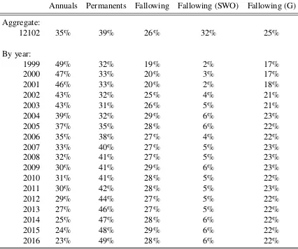
3.2 History of Crop Change . . . 58

3.3 Plot Level Summary Statistics . . . 60

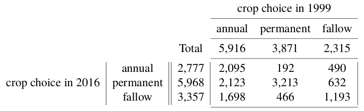
3.4 Crop Transition Matrix . . . 61

3.5 Moran’s I in Districts without Groundwater . . . 67

3.6 Determinants of Planting Permanent Crops . . . 73

3.7 Determinants of Planting Annual Crops in Water Districts without Ground-water before 2004 . . . 75

3.8 Determinants of Fallowing in Districts with Groundwater . . . 76

3.9 Robustness Check: Continuous Outcome Measure . . . 78

(9)

C h a p t e r 1

INTRODUCTION

Groundwater depletion has been a critical problem in dry regions like California. It leads

to environmental issues such as land subsidence, seawater intrusion, degradation of water quality, etc., thus causing significant economic losses. According to a recent report1, the cost of managing groundwater in the aquifer by recharge ranges from 90 to 1100 USD

per acre-foot, far below the cost of reservoir expansion (1700 to 2700 USD per acre-foot) and seawater desalination (1900 to over 3000 USD per acre-foot). Therefore, groundwater

depletion is not merely in the interest of environmentalists. Groundwater users can take

action themselves to avoid the huge cost that may be incurred in the near future.

Luckily, running out of groundwater is not the destiny of California water users. The water

table in Southern California basins has been stabilized in recent decades, despite a long history of decline. Most Southern California aquifers are managed through adjudication, a

form of self-governance that restricts average total extraction from the aquifer not to exceed

its sustainable yield.

Adjudication is expensive and slow. It can take decades for the water users to negotiate

the allocation of pumping rights and other management regulations. It is also expensive

to investigate the hydrology of the aquifer to determine the sustainable yield of the basin. Since water rights are usually determined based on historical use, information asymmetry

about each party’s past water consumption also presents. As a result, it is not surprising

that adjudication mainly succeeds in Southern California, where rapid urbanization has increased the users’ value of water and the willingness to pay for management.

No adjudication occurs in the Central Valley where the agricultural community consumes more than 90% of water. Due to the sparse interest among farmers, no one is willing to pay

(10)

for the cost of management even though the collective action can benefit all the users. In particular, farmers do not want to bear the cost to monitor. As a consequence, groundwater

basins in the Central Valley are still in open access today, and their water table keeps falling.

Without regulation, the commons problem is easily exacerbated by institutions that affect

the allocation of surface water, a substitute for groundwater. The farmers not only pump for

their own use. With well-defined surface water rights and a market for surface water trade, they are likely to sell their surface water rights to those without enough irrigation water

and pump more groundwater to compensate the water sale. In Kern County, groundwater

districts supply their surface water to districts without groundwater and pump more for their own use. The amount of extra pumping that is imputed to surface water sale accounts for

about 80% of the groundwater over-extraction in the county.

The open access groundwater system suffers more than just the commons problem. It is also vulnerable to other institutional arrangements that target to improve water use efficiency.

This is an example of the second-best scenario where the partially efficient water system does

not generate the second-best outcome. Implementation of a surface water market should take into account its unintended consequence on groundwater aquifer. A groundwater

regulation not only solves the commons problem, but also avoids the distortion caused by

the surface water market.

The optimal aquifer management requires a dynamic efficient groundwater extraction plan.

To implement that plan, the pumping rights and their allocation need to be carefully designed

to induce the efficient extraction and be incentive-compatible. In the rest of the thesis, I will discuss the adjudication of groundwater rights in Chapter 2, the surface water market

(11)

C h a p t e r 2

ADJUDICATION OF GROUNDWATER RIGHTS IN SOUTHERN

CALIFORNIA

2.1 Introduction

Recent studies of self-governance have brought new perspectives on how to solve common

pool resource (CPR) problems (Ostrom, 1990; Ostrom, 2002). A rich body of lab exper-iments (Messick, Allison, and Samuelson, 1988; Ostrom, Gardner, and J. Walker, 1994;

J. M. Walker et al., 2000) and field case studies (Berkes, 1986; Berkes et al., 1989a;

Os-trom, 1990; Blomquist, 1992; Casari, 20071) have confirmed that appropriators can devise regulations among themselves to manage the common pool. Outside authorities (such as

the government) and private markets, as suggested by the conventional theory of the CPR

problem2Hardin (1968), are not the only solutions to “the tragedy of the commons” (Ostrom and J. Walker, 2000).

Despite the growing consensus on the effectiveness of self-governance (Agrawal, 2001; Rahman, Hickey, and Sarker, 2012; Atkinson et al., 2014), the literature provides little

quantitative evidence of the success of private solutions (Tang, 1992; Lam, 19983). For this chapter, I assemble an original dataset from Southern California groundwater basins, conduct a cross-sectional analysis and demonstrate that self-governance does improve

sus-tainability.

Beyond sustainability, I also extend the general framework of CPR to a multi-period model with uncertainty in the availability of substitute resources. I analyze the dynamic efficiency

of different institutions depending on how the agents utilize the CPR as insurance against

demand and supply risk.

1_{The cases investigated in those studies include fishery (also lobster), wildlife hunting, forest management,} groundwater pumping, etc.

2_{Also see M. Olson (1965) for the discussion of the more general collective action problem.}

(12)

The context for this chapter is groundwater pumping in Southern California. Groundwater contributes a significant proportion of the state’s total water supply. It provides more

than one-third of water used by Californians in an average year and more than one-half in a

drought year when other sources (mainly surface water) are scarce4. In Southern California, groundwater basins account for nearly 35 percent of total water supply and almost 70 percent

of the local supply5.

Groundwater pumpers confront two layers of issues. First, in an unregulated basin,

com-petitive pumping leads to overdrafting and irreversible destruction of the basin’s storage

capacity. Second, it is unclear how to make joint use of groundwater and surface water efficiently (Zilberman and Lipper, 2002). Unlike surface water, the groundwater supply

is not sensitive to immediate weather condition. I argue that groundwater use is the most

efficient if pumpers save water in wet years and pump more during droughts. Their doing

so of course depends on incentives.

Two broad types of groundwater management exist in California. Most basins remain

unregulated. Within them, anyone can drill a well and pump groundwater. Some basins are managed in a different way. They have been adjudicated, meaning that the overlying

pumpers have arrived at a legal settlement to close the common pool and apportion the

pumping rights among themselves. We consider adjudication as a self-governing institution since the pumpers initiate the process and design the management rules among themselves.

Although the courts are involved, they are merely a third-party enforcement agency whose

authority is recognized by the pumpers.

Using a theoretical model, I analyze the sustainability and dynamic efficiency of the two

different institutions. I start by demonstrating that competitive pumping leads to more

extraction than the socially optimal level. I hypothesize that adjudicated basins are more likely to be sustainable than the unregulated ones – in simple terms, they suffer less ground

water level decline. In terms of dynamic efficiency, I argue that an optimal intertemporal

4_{See findings in the Sustainable Groundwater Management Act (SGMA) of California.}

(13)

groundwater-pumping pattern requires a certain level of counter-cyclicality6 to offset the variation of surface water supply. Due to the saving externality, competitive pumpers do not

have enough of an incentive to use the basin as a drought buffer. In my model, adjudication

generates an even smaller counter-cyclical pumping pattern than the competitive case.

My empirical findings confirm the claims that self-governing institutions can solve the CPR

problem. By comparing the changes of water levels of wells located in adjudicated and unadjudicated basins within the same period, I find that the self-governed systems are better

at preserving water levels. The panel data analysis also shows that groundwater use in

adjudicated basins is less counter-cyclical than unadjudicated ones. This result is consistent with the model, and verifies our concern that adjudication may have a problem with dynamic

efficiency.

I begin with some necessary background of groundwater basins and groundwater manage-ment in California. In Section 2.3, I present the dynamic model of pumping with uncertainty.

I will impose different institutions, and then solve for agents’ best responses. Section 2.4

contains the empirical analysis, which tests the hypotheses developed in Section 3. Section 2.5 summarizes my conclusion and discusses the broader implications of my findings.

2.2 Background

Groundwater basin as a common pool

Groundwater is generally stored in subsurface zones of saturated sediments called aquifers.

A groundwater basin is defined as an alluvial aquifer or a stacked series of alluvial aquifers with reasonably well-defined boundaries (nonwater-bearing material such as bedrock or an

underground displacement of rock such as a fault or divide) in a lateral direction and a

definable bottom7. Groundwater travels within an aquifer from areas of higher elevation towards areas of lower elevation. It may also flow into adjacent basin across underground

divides, but the confining boundary makes it much harder for water to leave than flow

(14)

within the aquifer (Heath, 1983). Although not completely isolated, each basin can be approximately treated as an isolated system, which is mainly affected by pumping from its

own aquifers8.

In a typical basin, groundwater is a renewable resource. As discussed in Karamouz, Ahmadi,

and Akhbari (2011), water enters a groundwater basin either by percolating through the

soil and overlying sediments or by flowing in from adjacent underground water systems. A certain amount of water may be “harvested” over regular intervals without impairing the

resource. This is the safe yield of the basin. The “annual safe yield” of a basin is roughly

its long-term average annual natural replenishment. Overdrafting in modest amount and for limited periods is unlikely to cause serious adverse consequence in most groundwater

basins. Persistent over-pumping, however, can make the sediments compact. Then, the

aquifer’s storage capacity may dwindle or even disappear. With extensive compaction, land

may subside, which causes serious problems for surface structures.

A basin satisfies the definition of CPR system as it generates finite water resources with one

person’s use negatively affecting others’ access to water. The negative externality occurs through two channels. First, water level declines increase pumping lift and imposes greater

cost on others. If the water level falls below a certain threshold, wells must be deepened or

replaced, pushing out those pumpers who cannot afford the capital investment. Second, if the outflow of water is not fully compensated by recharge, the storage space of an aquifer

may shrink. Water users then need to invest in expensive ground facilities such as reservoirs

for water storage (Carruthers and Stoner, 1981).

Groundwater rights and management regime in California

The groundwater rights system of California recognizes two different sets of water rights.

Overlying rights allow landowners to extract water from wells on their property.

Appro-priative rights are recognized mainly for water purveyors that deliver water to customers.

(15)

Although appropriative rights are generally subordinate to overlying rights, neither water right system specifies quantity or associated rules to prevent others from obtaining new

rights (Sawyers, 2005). As a result, every pumper is an unlimited groundwater right holder,

which makes it difficult to restrict extraction.

Prior to 2014 groundwater was not regulated by the State. The political power of counties

and municipalities to manage groundwater is uncertain, since basins generally do not respect county or municipal boundaries. Even for matters within the jurisdiction of local political

entities (regulation of well drilling), counties or municipalities rarely attempt to restrict

pumping9. In fact, through California’s history, local pumpers are always the primary decision-makers on groundwater issues. The California Legislature has repeatedly held

that groundwater management should remain a local responsibility (Sax, 2002). The most

recent legislation (SGMA 2014) requires basins to form their own groundwater sustainability

agencies, continuing its long stand of letting the users to solve their problem locally.

In adjudication, the most prominent path to groundwater management, local pumpers turn

to courts to settle disputes over how much groundwater can be extracted by each party. It starts when a suit is brought to adjudicate the basin (e.g. City of Pasadena v. City of

Alhambra et al.), but usually evolves to a situation in which each defendant’s answer to

the complaint is treated as cross-complaints against other defendants because of the mutual prescriptive nature of water rights conflict (Blomquist, 1992). The court helps defining the

limitation of resource and boundary of water rights community, but it requires the parties

to negotiate agreements among themselves. Therefore, each case of adjudication is a fully decentralized bargaining process. The court judgment is in fact a private contract among

the water users in the basin, with the court acting as the enforcement agency. In a typical

adjudication, the court rules on several matters10:

9_{Some counties or cities (for example the Venura County and the city of Beverly Hills) have ordinances} to regulate well permitting process or groundwater extraction. However, the regulating power is mainly on the public purveyors who have high value of water use and plenty of supplemental water resources.

(16)

1. who the extractors are;

2. how much each party can extract; and

3. who the watermaster will be to monitor and sanction the violation against the court’s

decree.

Adjudication is usually slow and costly due to the uncertainty about basin hydrology, the complexity of existing water right and the massive and diverse interests in the bargaining

process. It took seven years to adjudicate the Raymond basin, and more than ten years

passed in the first attempt for the Mojave river basins that ended in failure. Although adjudication is well understood by groundwater users in the state, it has hardly diffused to

north of the Tehachapi Mountains, leaving Southern California the unique field to examine

the influence of self-governance on CPR’s performance.

Next, I analyze a model of groundwater pumping.

2.3 A Model of Pumping under Uncertainty

There are N > 1 water users overlying a basin. Denote the agents by i = 1, ...,N. For simplicity, assume the water users are identical11. Each agent obtains revenue f(q)from “consuming”qunits of water. Depending on the type of the water user, “consuming” means selling the water if the agent is a water purveyor, or watering crops if the agent is a farmer.

The revenue function is increasing and concave.

There are two sources of water, surface and ground water. Surface water is available at a

price that depends on current condition (high in drought, low in rainy years). Denote the severity of drought asd. The unit price of surface water p(d)is an increasing function of the drought level.

(17)

Groundwater must be pumped. The cost of pumping has two components, the amount of extraction and the depth of the water table. When the water table falls, pumping lift in the

well increases and groundwater contains a larger quantity of dissolved solids. Both will

increase the pumping cost. Let the influence of water level be linear. The pumping cost takes the form: c(e) = le¯ , where edenotes the amount of extraction and ¯l is the average depth to the water in the well during the pumping process.

Water depth l changes with production and recharge. In the short run, natural recharge is negligible. The water level change in agenti’s well is only affected by her own extraction

ei. Therefore, we have the final water depthli = l0+ _se_wi wherel0denotes the water depth

before extraction andsw is the size of the well.

In the long run, water moves from high elevation to low elevation within the basin.

Fol-lowing previous economic studies (Gisser, 1983; Koundouri (2004)), I model the basin as a bathtub12. Long-term water level in the basin is determined by the total extractionE =Í

iei

and natural rechargeHduring the period. According to the bathtub condition, water depth is the same across the agents in the long run: l1 =l0+ Es−_bH wheresbdenotes the size of the

basin.

Assume the number of the agents is linear to the size of the basin: sb = sN where s is a positive parameter. The long-term change of water depth is l1− l0 = ei

sN +

Í

j,iei−H

sN .

Therefore, the larger the basin is, the less a single agent’s extraction contributes to the

overall water depth change.

For simplicity, I normalizesw = 1₂ ands =1. Leth= H_N. As a result, the short run average water depth in agenti’s well is ¯l = l0+ ei, and the long-term water depth in the basin is l1= l0+

Í

iei N −h.

(18)

In a static setting, agenti selects water consumptionqi and extraction ei to maximize her payoff:

max

qi,ei

f(qi) −c(ei) −p(d)(qi−ei) (2.1)

Henceforth, I only consider the solution with qi > ei. In this case, surface water is the marginal source, and agents will keep pumping until the marginal cost of groundwater

equals the surface water price. This assumption is reasonable in Southern California because nearly all communities use imported surface water every year13. Both equilibrium water consumption and extraction depend on the price of surface water:

qi = f0−1(p(d)); ei = p(d) −l0

2

Agenti’s optimal level of extraction changes with surface water price and starting level of water depth. Higher surface water price makes it more attractive to withdraw water from the basin; a larger water depth makes it more costly to pump. In the static case, individual

extraction is essentially a private process since the water level only changes locally over a

short period. The problems with competitive pumping arise for longer time horizons.

This chapter models the externality through increased future pumping cost. Since water

moves within the basin, the starting water depth next period is l1 = l0+

Í

iei

N − h. In a

multi-period situation, every agent receives the full benefit from current extraction, but only bears part of the future increased pumping cost. As a result, individual rational choice of

extraction leads to “over-pumping” of the basin.

Typically, there is another channel of externality caused by pumping. Given the finite

recharge rate of the basin, any agent’s extraction increases the possibility of overdrafting

and shrinkage of basin storage space. As the risk is also positively correlated with overall pumping, I shut down this channel in the modeling process. However, we will keep it in

mind when discussing the incentive of adjudication.

(19)

Another potential problem with competitive pumping is the failure to consider dynamic efficiency. Competitive agents have little incentive to save for future dry years since the

overall over-pumping will result a high pumping cost anyway. Intuitively, in an efficient

pumping scheme, users should pump less in wet years to save for dry years when the alternative surface water is very expensive. I employ a two-period model to study water

users’ intertemporal pumping decisions. Weather d is realized in the beginning of each period (t = 1,2), as well as the surface water price p(d) and natural replenishment H(d) as a function of the drought level. H0(d) < 0 and h(d) = H_N(d). l0 is the water depth at the beginning of Period 1; l1 is the water depth at the end of Period 1 and beginning of

Period 2. Agents choose water consumption and extraction for each period after observing the weather condition. The discount factor is 114.

State of nature

The first case I will explore is the state of nature when no governing agency controls

pumping. Each agent extracts based on her own cost-benefit analysis. The optimization problem is solved backwards. In Period 2, agenti’s maximization problem is:

max

q2i,e2i

f(q2i) −c(e2i) − p(d2)(q2i−e2i) (2.2)

where c(e2i) = (l1 + e2i)e2i. I only consider the case when parameter values yield the interior solution with positive surface water purchase. Let the value function of Period 2 be

V2i. The Period 1 problem is:

max

q1i,e1i

f(q1i) −c(e1i) −p(d1)(q1i−e1i)+_E_d[V2i] (2.3)

(20)

wherec(e1i)= (l0+e1i)e1i. The solution to the above two-period problem is:

qn_1i = f0−1(p(d1)); q_2in = f0−1(p(d2))

en_1i = 2N p(d1) −h(d1) − (2N−1)l0−M

4N−1 ; e

n 2i =

p(d2) −l0− E₁n

N +h(d1)

2

E_1in = 2N p(d1) −h(d1) − (2N−1)l0−M

4− _N1 ; E

n 2 =

N[p(d2) −l0+h(d1)] −E₁n

2

whereM = Ed[p(d)].

Any reduced extraction in Period 1 will increase water level in Period 2. Due to the structure of the cost function, a dynamic efficient pumping arrangement will encourage an optimal

amount of saving by each agent. However, in a competitive case, an agent bears the full

cost of saving but only receives part of its benefit since raising the water table generates a positive externality to others. Therefore, in the model, lack of regulation not only leads to

more pumping than is sustainable, it also fails to be dynamic efficient. I will validate this

argument by a comparison with the socially optimal pumping strategy.

Social planner’s problem

An opposite scenario to the competitive pumping allocates pumping decisions to a central

authority. Uncertainty to weather remains, but the central planner has all the information

she needs and optimizes as social planner. Again, there is a two-period problem:

Period 1: max

q1i,e1i,i=1,. . . ,N Õ

i

{f(q1i) −c(e1i) −p(d1)(q1i−e1i)+_Ed[V2i]} (2.4)

Period 2: max

q2i,e2i,i=1,. . . ,N Õ

i

{f(q2i) −c(e2i) −p(d2)(q2i−e2i)} (2.5)

The Period 2 social planner’s problem is the same as the individual agent’s problem, since

any agent’s extraction does not affect others’ pumping cost and the world ends at the end of

(21)

of pumping. The solution to the two-period problem is:

q_1isp= f0−1(p(d1)); q_2isp = f0−1(p(d2))

e_1isp= 2p(d1) −h(d1) −l0−M

3 ; e

sp 2i =

p(d2) −l0− E₁s p

N +h(d1)

2

E_1isp= N[2p(d1) −h(d1) −l0−M]

3 ; E

sp 2 =

N[p(d2) −l0+h(d1)] −E sp 1

2

WhenNis large enough,E₁n > E₁spis approximately equivalent to[M−p(d1)]+[M−l0+

2h(d1)] > 0. M−l0+2h(d1) > 0 always holds by construction. Since M = Ed[p(d)], on

expectation, M −p(d1) = 0. Therefore, ex ante, competitive pumping leads to a depleted basin. In the short term, it is possible forp(d1)to be very high due to extremely dry weather.

A dynamic efficient pumping scheme may require the agents to pump even more than the competitive level and compensate by reduced extraction in the future. This confirms our

speculation that competitive pumping does not provide agents with sufficient incentives to

save water for dry years.

Adjudication

Although a social planner can achieve maximal welfare for the group of pumpers as a whole,

it is not always feasible to implement an optimal scheme. In a world with heterogeneous

pumpers, the central authority may not have the appropriate information to decide the pumping allocation15. What’s more, it is not clear who can play the role of social planner in particular because of agency problems16. Lam (1998) has shown that government systems actually do worse than self-governing irrigation systems in Nepal. The same concern exists among Southern California pumpers (Blomquist, 1992). Adjudication, as a form of

15_{In Gordon (1954), the author mentioned the failure of the international fishery agreement between the} United States and Canada that established a fixed-catch limit during the early 1930s. The limit led to a competitive race for fish and over-investment in capital. A similar problems also arose in the Canadian Atlantic Coast lobster-conservation program. To the contrary, also mentioned by the author, in a few places the fishermen have successfully reduced fishing gears and improved income by banding with each other and setting up rules regulating their own operations.

(22)

self-governance, may also be more acceptable to the local pumpers than the centralized regulation by the state.

Pumpers rely on adjudication to achieve two main outcomes. First, it protects the basin from overdrafting by setting the total annual pumping rights equal to the long-term safe

yield of the basin. Second, it avoids competition between the pumpers by assigning an exact

amount of pumping rights to each of them.

As each basin devises its own rules, the flexibility of adjudicated rights varies across

adjudications. A key source of variation is the benchmark used to decide the pumping

rights R. Some basins target the long-term average yield of the basin, i.e. R = _Ed[H(d)].

Others use a varying annual yield17, the so-called operating safe yield, to determine pumping right each year, i.e. R(d) = H(d). Both adjudication rules can achieve sustainability, but they have different short-term implications.

A second dimension of difference worth exploring is the option to save. Some basins allow

pumpers to store any unused pumping rights and increase their future rights accordingly.

Others strictly execute the assigned pumping allocation, and impose replenishment fees for over-pumping immediately. The savings option can influence agents’ intertemporal

pumping decisions. In my model, any adjudication achieves sustainability by assumption,

but it remains uncertain how the adjudication rules affect dynamic efficiency. I will examine the two dimensions of flexibility by considering the 2×2 cases: long-term average yield

versus operating safe yield, and savings versus no savings.

Long-term average yield without savings

Using long-term average yield and not allowing savings seem to be the most rigid type

of adjudication. Appropriators face the same upper bound of pumping r = _NR in each period independent of the weather18. In Period 2, the agent faces a constrained optimization

17_{To do so, some technical advisor estimates the yield of the basin in next water year before it starts. The} estimation is taken as the operating safe yield.

(23)

problem:

max

q2i,e2i

f(q2i) −c(e2i) −p(d2)(q2i−e2i) s.t. e2i ≤r (2.6)

The value function of Period 2 is not smooth at the point that the constraints bind. Taking into

account the expected value in Period 2, the agent solves another constrained optimization

problem in Period 1:

max

q1i,e1i

f(q1i) −c(e1i) −p(d1)(q1i−e1i)+Ed[V2i] s.t. e1i ≤ r (2.7)

If neither constraint binds, the problem is the same as competitive pumping. In this chapter, we are interested in cases where adjudication is not trivial. Therefore, I only consider the

case where both constraints bind. This is true when natural recharge or adjudicated pumping

rights is so limited that, even at the boundary, the marginal cost of pumping is too low to generate any incentive for saving. Water use and extraction in each period are:

q_1il,ns = f0−1(p(d1)); q_2il,ns = f0−1(p(d2))

el_1i,ns =r; el_2i,ns =r

E_1il,ns = R; E₂l,ns = R

Without doubt, the rigid adjudication rules lead to rigid pumping decisions. Extraction is

constant in each period irrespective of surface water availability.

Operating yield without savings

A modification to the rigid allocation above is to use operating yield as the benchmark when

deciding annual pumping rights. However, without savings accounts, agents still do not

have an incentive to smooth pumping over time. Compared with the first case, the constraint to the maximization problem now varies according to the realized weather condition in the

period:

Period 1: max

q₁_i,e₁_i f(q1i) −c(e1i) −p(d1)(q1i−e1i)+Ed[V2i] s.t. e1i ≤ r(d1) (2.8)

Period 2: max

q2i,e2i

(24)

Again, I only consider the case when both constraints bind. Since the basin does not allow savings, the overall extraction only reflects the change of natural recharge. Water use and

extraction in each period are:

q_1io,ns = f0−1(p(d1)); q_2io,ns = f0−1(p(d2))

eo_1i,ns = H(d1)

N ; e

o,ns 2i =

H(d2) N E_1io,ns = H(d1); E₂o,ns = H(d2)

Although it seems more flexible, I argue that using operating yield without a savings

account actually decreases the overall welfare. Since H0(d) < 0, indeed in the constant annual extraction program, groundwater use is less than recharge in wet year and more than recharge in dry years. With operating yield extraction, groundwater use will be less in dry

years and more in wet ones. Therefore, agents actually buy more surface water in dry years

when it is expensive and less in wet years when it is cheap. The pro-cyclical pattern of groundwater recharge actually undermines the basin’s function as drought buffer.

So far, neither adjudication rule provides the agents with the right incentive to use

ground-water as drought insurance. That is why it is important to have a savings option with adjudication.

Long-term average yield with savings

In a two-period model with savings allowed, each agent does the cost-benefit calculation

with an overall budget constraint. The constrained optimization problem is:

Period 1: max

q1i,e1i

f(q1i) −c(e1i) −p(d1)(q1i−e1i)+_E_d[V2i] (2.10)

Period 2: max

q2i,e2i

f(q2i) −c(e2i) −p(d2)(q2i−e2i) s.t. e2i ≤ 2r−e1i (2.11)

Since the total budget of extraction is fixed, the agent smooths her pumping over two periods

(25)

solution to the two-period problem is:

q_1il,s = f0−1(p(d1)); q_2il,s = f0−1(p(d2))

el_1i,s = N[p(d1) −h(d1) −M]+(4N−2)r

3N−1 ; e

l,s

2i = 2r −e l,s 1i

E_1il,s = N[p(d1) −h(d1) −M]+(4N−2)r

3−1/N ; E

l,s

2 =2R−E l,s 1i

Given savings account, pumpers are willing to save in the first period if the price of surface water is low (e_1il,s decreases withp(d1)).

Operating yield with savings

The most flexible case is using operating safe yield as adjudicated rights and allowing savings

at the same time. When pumping rights depend on realized weather condition, pumpers are

assigned more pumping allocation in wet years than in dry years. The extraction budget is not fixed ex post, motivating the agent to choose the two periods’ pumping in a way that

not only takes into account the expected surface water price, but also the expected future

pumping allocation. The constrained optimization problem is:

Period 1: max

q1i,e1i

f(q1i) −c(e1i) −p(d1)(q1i−e1i)+_Ed[V2i] (2.12)

Period 2: max

q2i,e2i

f(q2i) −c(e2i) −p(d2)(q2i−e2i) s.t. e2i ≤

H(d1)

N +

H(d2)

N −e(2.13)1i

The solution to this problem is similar to the last case:

q_1io,s = f0−1(p(d1)); qo_2i,s = f0−1(p(d2))

e_1io,s = N

[p(d1) −h(d1) −M]+(2N −1)( H(d₁)

N +r)

3N−1 ; e

o,s 2i =

H(d1)

N +

H(d2) N −e

o,s 1i

E_1io,s = N

[p(d1) −h(d1) −M]+(2N −1)(H

(d1)

N +r)

3−1/N ; E

o,s

2 = H(d1)+H(d2) −E o,s 1i

Adjudication here also generates an incentive for saving, but when compared with the

(26)

is ∂E

s p

1

∂p(d1) =

2N

3 . That is always greater than ∂E₁o,s ∂p(d1) =

N

3−1/N, the derivative when pumpers

are managed by adjudication with a savings account. The externality still exists since one

agent’s saving will raise everyone’s water level in the second period. Adjudication may

successfully limit the amount of extraction and keep the water level stable, but we still have an unsolved problem of how to provide agents with a strong enough incentive to save in wet

periods.

Extensions

The simple two-period model has its limitations. The fact that pumping ends in Period 2 may be insufficient for a full comparison of dynamic efficiency across institutions. In the

real world, savings accounts can last much longer than two periods, increasing the agents’

incentive to save. In addition, the Period 2 equilibrium extraction is solved under a “use it or lose it” situation. That is not a problem when the quantity of pumping rights is specified.

However, in looking at the social planner’s optimum, something is lost because agents pump

more in Period 2, which has an unexpected effect on their Period 1 pumping plan.

Chapter 4 extends the two-period model to an infinite horizon problem. Both sustainability

and dynamic efficiency have a different implication in the infinite horizon game than the two-period model. In the steady state, the expected annual extraction from the basin should

be equal to its long-term recharge rate under any institution, so sustainability is not defined

based on the amount of pumping. Instead, lack of sustainability is associated with a lower steady state water level, which indicates that the basin is exposed to higher risk of depletion.

Since the competitive pumpers always have larger incentive to extract than the social planner,

the steady state water level under the state of nature should be lower than the socially optimal

level. In addition, during adjudication pumpers can select any water level to maintain by scheduling a controlled overdraft or artificial replenishment. The steady state water level

in an adjudicated basin should be close to the socially optimum to achieve larger overall

(27)

As for dynamic efficiency, it depends on how agents allocate the same amount of steady state extraction across different weather conditions. The social planner’s incentive to save

in wet years as drought insurance does not change; the agents have an incentive to save but

they still suffer from the externality. The competitive case is more complicated. On one hand, pumpers react to the surface water price with little incentive to save; on the other

hand, the amount of extraction depends on the water level which is much lower during a

drought cycle due to lack of natural recharge. As a result, I anticipate that adjudication still have a problem with dynamic efficiency, but it remains unclear how adjudication works

compared with the state of nature.

As for this chapter, I will put aside the difference between this model and an infinite horizon

game. In next sub-session, I discuss the hypotheses drawn from the simple two-period

model. I will test these hypotheses in the next section.

Hypotheses

Two sets of hypotheses can be drawn from the equilibrium analysis:

Hypothesis 2.1 (Sustainability) As adjudication generally limits the maximal amount of extraction, I expect adjudicated basins to pump less than unadjudicated ones and hence are more likely to maintain groundwater resources.

The other hypothesis is related to the dynamic efficiency. I expect the optimal mechanism to have some responsiveness to changing weather conditions. Once again, the first derivative

of Period 1 total extraction to the price of surface water is a measure of dynamic efficiency19. It shows to what extend agents adjust their pumping plan according to the availability of supplemental water resources.

(28)

The first derivatives of Period 1 total extraction over surface water price are as follows:

∂E₁n ∂p(d1) =

2N 4− _N1 ;

∂E₁s p ∂p(d1) =

2N 3 ;

∂E₁l,ns ∂p(d1) =

∂E₁o,ns ∂p(d1) =

0; ∂E l,s

1 ∂p(d1) =

∂E₁o,s ∂p(d1) =

N

3− _N1 (2.14)

They satisfy:

∂E₁sp

∂p(d1)

> ∂E

n 1

∂p(d1)

> ∂E

l,s 1

∂p(d1) =

∂E₁o,s

∂p(d1)

> ∂E

l,ns 1

∂p(d1) =

∂E₁o,ns

∂p(d1)

(2.15)

As a result, I argue that neither the state of nature nor adjudication generates enough counter-cyclicality of pumping. Within the adjudicated basins, adjudication without the option to

save is rigid, because agents do not take into account the price of surface water at all. In the

hypothesis of dynamic efficiency, I put adjudication with a savings account in one category and without in another category. Since we only observe the state of nature and adjudication

in Southern California,20I compare the relative counter-cyclicality of those two institutions:

Hypothesis 2.2 (Dynamic efficiency) The state of nature generates a larger counter-cyclical pumping pattern than adjudication, and among the adjudicated basins, those without a savings option do not have enough counter-cyclicality.

2.4 Empirical Analysis

The empirical basis for this study is a collection of depth to water (henceforth well depth)

data for 87 wells in 33 Southern California basins. Under the assumption that an aquifer is

like a bathtub, the hydrology of a basin satisfies the formula:

∆Water Level×Size of Aquifer= Total Recharge−Total Extraction (2.16)

Therefore, the change in the water level in a basin is a monotonic function of recharge and extraction normalized by the size of the basin. In reality, the bathtub condition generally

does not hold, so we do not have a unified measure of water level change in one basin. As

(29)

an alternative, I look at individual wells in each basin and use the change of well depth as the measure of water level change.

There is no clear geological definition for Southern California as a whole. In this study, I follow the classifications of the DWR’s Southern Region Office and include three

hydrolog-ical regions: South Coast, South Lahontan, and Colorado River. Selection of those regions

is reasonable since all adjudicated basins, except for some coastal ones, are in this area21. DWR identifies 214 basins or subbasins in Southern California, among which I only select

the 59 basins that produce more than 3000 Acre-feet (AF) groundwater per year22. The largest basin produces as much as 342,000 AF of groundwater each year, so the lower limit excludes a large number of extremely small basins where a single dominant agent may bear

the cost of collective action.

Because of data limitations23, the period of study is 2000 to 2015. Not all wells have 16 years of well depth readings. For each basin, I only pick the wells with 14 or more years’

observation from 2000 to 2015. I keep at most 3 wells for one basin if that basin has more

than 3 wells satisfying our requirement. We end up with 33 basins and 87 wells in our sample. Most basins have 2 or 3 wells.

Table 2.1 illustrates the representativeness of our sample. According to the p-values from

the t-tests, our sample does not have a statistical significant difference from other large basins (> 3000 AFY) in terms of size, share of agricultural land and population density.

It does include more adjudicated basins, consistent with the fact that adjudicated basins

are more likely to monitor their water levels. The comparison of the sample basins and the excluded small basins imply that the basins with less than 3000 AFY have significantly

different basin characteristics. In particular, they are smaller and less populated, confirming

21_{Coastal basins have a different incentive to adjudicate than inland ones. They are more likely to be} threatened by seawater intrusion instead of increasing pumping cost.

22_{The estimates are from DWR California Groundwater Update 2013.}

(30)

our concern that those basins may have a smaller group of pumpers and thus a different groundwater use situation.

Basins in the Sample Other >=3000 AFY Other South Cal. Basins

Number 33 26 181

Mean Mean Mean difference p-value Mean Mean difference p-value

Fraction of adjudication before 2000 0.52 0.23 -0.28 0.03 0.06 -0.45 0.00

Basin size (acres) 135545.27 149605.15 14059.88 0.78 87051.51 -48493.76 0.10

Fraction of ag. land 0.18 0.10 -0.08 0.18 0.03 -0.15 0.00

[image:30.612.105.541.126.209.2]

Population density (per acre) 3.30 2.27 -1.03 0.33 1.05 -2.25 0.00

Table 2.1: Representativeness of the Estimated Sample

Well depth change is our outcome variable and the two main equations we want to estimate

are:

yjit = α1+β1Ai+θ1zi+σ1t+1jit (2.17)

yjit = α2+β2Ai+γDt+δAi×Dt+θ2zi+σ2t+2jit (2.18)

yjitis change of well depth for well jin basiniat periodt. Aiis a dummy which equals to 1 if the basin is adjudicated before 2000 and 0 otherwise. A_iis a vector of institution dummies, which equals to(1,0)if the basin is adjudicated before 2000 with a savings account,(0,1)

if the basin is adjudicated before 2000 without a savings account, and (0,0)if it has not

been adjudicated before 2000. Dt is a weather dummy which equals to 1 if the period t

is a dry period, and 0 otherwise. Ai× Dt is the cross-term to test the marginal effect of

institutions on water level changes during different weather cycles (dynamic efficiency);zi

is a vector of control variables including relevant basin characteristics;σt is the time fixed

effect; and jit is the error term. Because error terms for wells from the same basin are

generally correlated, they are clustered at the basin level in the regression analysis.

As for the institution variable, the DWR has established the Adjudicated Basins Annual

Reporting System where we can find the names of the adjudicated basins and the terms of

adjudication. There were 27 court adjudications in California through 2015. Twenty of them occurred in Southern California, and they cover 30 basins. According to Table 2.2,

(31)

before 2000 and three afterwards. To avoid the identification problem that arises in our sample because a basin may be unadjudicated before a certain year and then adjudicated

afterwards, and to eliminate the immediate effect of adjudication, I use a dummy variable

indicating whether a basin is adjudicated before 2000 as our main institution variable24. Through the division of basins according to their institution choice at 2000, I compare those

basins that are always adjudicated in our sample period with the rest.

For each adjudicated basin, I use the adjudication documents to identify the specific rules

adopted by that basin. Some adjudicated basins allow carry-over of unexercised pumping

rights while some do not give credit for that. I code the basin as adjudicated with a savings account if its adjudication rule allows for storage of unused pumping rights; otherwise, I

code the basin as adjudicated without a savings account. Twelve out of 17 adjudicated

basins allow savings.

The primary source of well depth data is California Statewide Groundwater Elevation

Monitoring Program; the Water Data Library of DWR also provides well depth observations.

I also ask water agencies directly for well monitoring data if CASGEM contained less than three qualified wells in their basin. For each well in our sample, we have scattered readings

of water level on dates casually drawn from the 16-year period. Difference between any

two readings is one observation of water level change25. For instance, the water level on January 1st, 2005 minus the water level on January 1st, 2004 is an observation of one-year

water level change. A positive water level change reflects an increase of water table and a

negative water level change a decline. In the tests, I only use water level changes over one, two, three or four full years to get rid of seasonality.

The unit of observation in the regression analysis is an individual well. We have a panel

dataset since in principle we can observe water level changes of all wells on any time

24_{In our sample, all adjudicated basins were adjudicated before 2000 except for one in 2015. Even if we} use the exact treatment (adjudicated or not), our empirical results will not change too much.

(32)

interval between 2000 and 2015. For instance, there should be 365×1526observations of 1-year water level change for each well during our sample period. Unfortunately, water level

observations occur at low frequency, and we do not always have two readings at a distance

of 1 year. We end up with fewer observations than the theoretical number, even when I relax the definition of 1-year water level change to the change between 12±1 months27.

Table 2.2 presents the summary statistics of the outcome variables that I use in the regression analysis. We have 9172 observations of 1-year well level change in our regression. Among

them, nearly a half are from the adjudicated basins, which is close to the fraction of

adjudication basins over all sample basins. I also compute 2-year, 3-year and 4-year water level changes. The sample is quite balanced since there are always more than 45%

observations from the adjudicated basins.

Adjudicated before 2000 Not Adjudicated before 2000 Total

Mean(not adj.) - Mean(adj.) p-value

Number Mean Number Mean Total Mean

Basin 17 16 33

Well 45 42 87

Change of water level (feet)

1-Y 4314 -0.52 4858 -1.87 9172 -1.23 -1.35 0.00

2-Y 3916 -0.24 4540 -4.15 8456 -2.34 -3.91 0.00

3-Y 3562 -0.74 4228 -5.81 7790 -3.50 -5.07 0.00

4-Y 3221 0.65 3927 -7.52 7148 -3.84 -8.18 0.00

Population density (per acre) 4769 3.02 5153 2.67 9922 2.84 -0.35 0.00

Fraction of ag. land 4769 0.04 5153 0.48 9922 0.27 0.44 0.00

Drought index 4769 -1.86 5153 -1.90 9922 -1.88 -0.04 0.59

Precipitation (inches) 4749 0.68 4986 1.01 9735 0.85 0.32 0.00

[image:32.612.110.539.342.447.2]

Note: The unit of observation is well*date.

Table 2.2: Summary Statistics

P-values from the t-tests of water level changes in the adjudicated and unadjudicated basins indicate that for all time intervals I examine, the adjudicated basins have experienced smaller

water level decreases compared with unadjudicated ones. This suggests that adjudication

does lead to improvement in sustainability. For example, the mean differences imply that the water level drops in the adjudicated basins is on average 1.4 feet less in 1-year interval,

3.9 feet less in 2-year interval and 8.2 feet less in 4-year interval28. The difference is

26_{The water level readings are at the daily level. From 2000 to 2015, we can find 365}_×_{15 pairs of dates} that are at a distance of 1 year. The difference of water levels between each pair of dates is one observation of one year water level change.

27_{I also allow 30-day flexibility for two-, three- and four-year intervals.}

(33)

significant both statistically and economically. On average, well levels drop 1.9 feet in the unadjudicated basins each year, while the wells in the adjudicated basins drop 62% less. If

we look at 4-year intervals, well levels in the unadjudicated basins on average drops 7.5 feet

within 4 years, while they actually increase 0.7 feet in the adjudicated basins.

Table 2.2 also reports the mean of population density, fraction of agricultural land, Palmer

drought severity index (PDSI) and monthly precipitation for all observations. The first two

variables are at the basin level. DWR divides California into Detailed Analysis Units (DAU) by which it estimates population and size of agricultural land annually. For the purpose

of our study, I match DAUs to each basin. There are cases that one basin overlies several

DAUs or several basins overlie the same DAU. For each basin, I add up estimates from all DAUs it overlies. Then I calculate the annual growth rate of population and agricultural

land using the sums. As I obtain 2010 population and agricultural land size for each basin

from another data source (DWR 2013 Update), I apply the growth rate to the 2010 data, and get an annual measure of population and agricultural land size for each basin. The unit

of population density is person/acre. As the data shows, on average, the adjudicated basins

are more populated and have a smaller proportion of land in agriculture.

The last two variables concern the weather. PDSI is an index that uses temperature and

precipitation data to estimate relative dryness. It is at monthly level and only published for

two broad regions: Colorado River/South Lahontan and South Coast. As a result, there is very little variation of PDSI across the basins. Therefore, I merely use it to define drought

and wet cycles over Southern California. I employ monthly precipitation data at the basin

level to control for basin specific weather conditions. The PDSI data I use in the study comes from the National Centers for Environmental Information, and the precipitation data

mainly comes from the California Irrigation Management Information System (CIMIS).

CIMIS has monthly-accumulated precipitation information for various stations. I associate each basin with the closest station and assign the precipitation figure from that station to the

basin. A complementary source comes from the California Data Exchange Center, which

(34)

may not start until after 2000, we have fewer observations with precipitation data than with other control variables. In general, the drought index does not show any difference between

adjudicated and unadjudicated areas, but the more detailed precipitation data shows that on

average the adjudicated basins have less rain than the unadjudicated ones.

Two coefficients from the two estimation equations are of particular interest for this research. β1measures the average effect of adjudication over the changes of water level across wells

from different basins and across different dates. According to Hypothesis 2.1, β1should be

positive since the adjudicated basins should have greater water level changes due to their

limits on extraction.

The other coefficient we care about isδ = (δ₁, δ₂). As the coefficients of the cross-terms of institution and drought dummy,δ1andδ2measure the effect of institution over the dry-wet

year difference of water level changes. The benchmark for the difference-in-difference analysis is counter-cyclicality of the unadjudicated basins, where the agents only react to

surface water price. According to Hypothesis 2.2, adjudication with a savings account

should be less counter-cyclical than the competitive case, or in other words, it should have a greater dry-wet year difference of water level changes. Furthermore, adjudication without

a savings account is expected to result a flat extraction pattern, with an even greater dry-wet

year difference. As a result,δ1should be positive andδ2should be greater thanδ1.

There is a potential problem with endogeneity because basins with severe overdraft might

be forced to adjudicate. Even when we choose the institution variable so that the treatment

happens before the sample period, we cannot ensure the underlying conditions causing the overdraft do not persist. Omitted variables such as precipitation and urbanization rate

might, for example, cause the selection bias in our estimation. A basin with less rain usually

has less natural recharge to the aquifer, but it is also more likely to experience drought and then adjudicate. Similarly, a more urbanized basin will have an easier time transferring the

adjudication cost to water users, and the urbanized area also has different water demand and

(35)

I use accumulated precipitation, growth of population density and growth of agricultural land ratio to account for the potential effects of weather and human activity. The selection

bias may still exist even after controlling for those three variables. However, since a basin

with higher propensity to be adjudicated is also more likely to suffer from the factors that cause water level decline, the selection effect, if any, should only bias our estimation results

downwards. Therefore, I can safely draw conclusions from the estimated coefficients despite

of the endogeneity issue.

In Table 2.3, I test the effect of adjudication over water level changes. Control variables

for the basin-level characteristics are included. The effect of adjudication becomes larger than indicated by the summary statistics in all time intervals after adding the controls. For

instance, the adjudicated basins now on average experience 0.7 feet increase of water level

in one year compared with 1.9 feet drop in the unadjudicated basins. Precipitation has a

positive effect in that 1 inch more precipitation in a year raises the water level up about 0.48 feet.

Both population density and agricultural land ratio growth lead to lower water level, implying both urban and rural water use have a negative effect on water level compared with places

with less human activities. In 1 year, a one standard-deviation increase of population

density growth leads to 0.75 feet decline of water level; a one standard-deviation increase of the change of agricultural land ratio leads to 1.3 feet fall of groundwater. Both effects

are significant in magnitude. One may worry that population density and the change in the

agricultural land ratio work in opposite directions. I also run regressions with only one of the two variables. The coefficients only change little, implying collinearity is not a concern.

The test of sustainability confirms the effectiveness of adjudication. Even without a central

planner or privatization, the agents within a basin can effectively regulate themselves and protect the basin from overdrafting. The role of self-governance on sustainability is crucial.

Without adjudication, basins on average experience decline of water level, while those

(36)

(1) (2) (3) (4)

Water level change 1-year 2-year 3-year 4-year

Adjudication before 2000 2.621** 7.533*** 9.445*** 14.43***

(1.098) (2.119) (3.012) (3.800)

Precipitation 0.482* 0.564** 0.523** 0.502***

(0.249) (0.231) (0.204) (0.181)

Population density change -19.79*** -20.42** -10.02 1.315

(7.210) (8.154) (7.880) (8.960)

Agricultural land change -139.2** -37.71 -196.6*** -83.74

(58.150) (35.620) (52.250) (79.860)

Constant -6.581** -15.99*** -22.53*** -30.33***

(2.879) (5.489) (7.656) (9.297)

Observations 8,771 8,036 7,364 6,729

R-squared 8.5% 14.5% 16.7% 16.9%

[image:36.612.136.515.76.380.2]

Note: Robust standard errors in parentheses are clustered at basin level. *** p<0.01, ** p<0.05, * p<0.1

Table 2.3: Effect of Adjudication on Water Level Change

Another hypothesis that I test is the dynamic efficiency of the adjudication rules. Since the

cyclicality of pumping results from the intertemporal decisions of the agents, we do not want to disturb the estimation by including periods with overlapping dates. Instead, I divide

the whole sample period into 3 drought cycles (2001-2004, 2007-2009 and 2012-2015)

and two wet cycles (2005-2006 and 2010-2011)29. I run panel analysis on the five cycles to check the marginal effect of institution on water level change under different weather

conditions.

Since there are not too many variations of adjudication rules in terms of savings account, in the first two columns of Table 2.4, I pool the adjudicated basins as one category. The

(37)

(1) (2) (3) (4) Depend Variable: water level change during hydrological cycles

Adjudication before 2000 3.785*** 2.507** (1.187) (1.164)

Adjudication before 2000 & Savings 4.168*** 3.503*** (1.215) (1.183) Adjudication before 2000 & No Savings 8.321*** 8.563***

(1.265) (1.228) Dummy for drought cycle -0.727 -13.01*** 0.581 -11.24***

(2.181) (2.371) (2.152) (2.328) Adjudication before 2000 X Dummy for drought cycle 8.911*** 7.868***

(1.751) (1.702)

Adjudication&Savings X Dummy for drought cycle 2.699 -0.0889 (2.348) (2.282) Adjudication&NoSavings X Dummy for drought cycle 4.461*** 0.989

(1.382) (1.361) Length of the cycle -13.34*** -2.411 -11.47*** -0.555

(1.461) (1.642) (1.454) (1.633) Precipitation 0.333*** 0.230*** 0.336*** 0.244***

(0.0250) (0.0254) (0.0256) (0.0257) Population density change 12.31*** 8.229** 7.923* 2.356

(4.219) (4.098) (4.310) (4.199) Agricultural land change 153.5*** 13.37 102.6*** -43.82

(34.64) (35.18) (32.99) (33.77) Constant 21.31*** 4.479 16.02*** -1.305

(2.923) (3.207) (2.799) -3.085

Cycle fixed effect N Y N Y

Observations 2,404 2,404 2,404 2,404 R-squared 16.3% 21.9% 16.2% 21.8%

[image:37.612.120.536.105.463.2]

Note: Robust standard errors in parentheses *** p<0.01, ** p<0.05, * p<0.1

Table 2.4: Effect of Institution on Cyclicality of Groundwater Extraction

effect of institution persists. Adjudication before 2000 results in higher water level. The

estimated coefficient for the cross term is positive, indicating that the difference of water

level change between dry and wet cycles is 6.7 feet larger in the adjudicated basins compared with the unadjudicated basins. So, the adjudicated basins do have a less counter-cyclical

groundwater use pattern than the unregulated ones.

Column 3 and 4 present the estimation by dividing the adjudicated basins into those with a

savings account and those without. The effect of adjudication remains. The sign of cross

(38)

adjudication without a savings account is statistically significant. The coefficient for the cross term of adjudication with a savings account is smaller than the coefficient for the cross

term of adjudication without a savings account, indicating that adjudication rules with a

savings option generate greater counter-cyclicality than the rigid rules.

Several issues remain unsolved for Table 2.4. Both the population density change and

agricultural land ratio change have signs that are the opposite of our expectation. Also, after clustering the error term at the basin level, we lose all significance. A better specification

of the estimation model is needed to address those issues.

2.5 Conclusion

A rich body of literature has documented self-organized governance on CPR systems around the world. In this chapter, I analyze groundwater management in Southern California

and confirm the effectiveness of self-governing institutions in solving the CPR problem.

Through adjudication, pumpers in the same basin arrive at a contract that specifies the exact amount each pumper can extract from the basin, as well as rules to monitor and sanction

the violations. By looking at water depth of wells located in different basins, I show that

the adjudicated basins have greater water level increase or smaller water level decrease than those unregulated ones within the same time period.

My findings have significant real-world implications. Since Elinor Ostrom’s pioneering

work (Ostrom, 1990; Ostrom, 2002), adjudication of groundwater rights has been considered as a major solution to CPR problem in groundwater basins. In the important case of

California, however, this institution rarely diffused to the north of the state. The reason

may be more complicated stakes in water rights (for instance in the Central Valley). If so, then my quantitative measure of the effect of adjudication can resolve the uncertainty that

the agents face weighing between the status quoand the legal settlement. The evidences found in this chapter will help the advocates of self-governance and accelerate institutional change.

(39)

self-governing institutions in terms of the dynamic efficiency of the CPR system. One concern raised by this chapter is that adjudication does not necessarily enhance the dynamic

efficiency of groundwater use. Allowing flexibility in adjudication rules can provide an

incentive for the agents to save water in wet years, but adjudication in general generates smaller counter-cyclical pumping pattern than the unregulated state. The fact that

indi-viduals governing the CPR may not have enough of an incentive to develop an efficient

intertemporal appropriating plan suggests it is worth weighing the trade-off between self-governance and other type of institutions more carefully. Moreover, institutional designers

may need to think about the proper mechanism if dynamic efficiency matters a lot for welfare

of the community.

A problem remains open: why is adjudication so slow to diffuse. Since the first adjudication

(Raymond Basin 1944), only 30 out of 214 basins have adjudicated in Southern California

and less than a handfull elsewhere in the State. Given the large benefit it brings, it is urgent to figure out why pumpers in some basins organize themselves and why they fail to do so

in other place. The study has to go back to the early stage when the adjudications actually

occurred. Work by Ostrom and Blomquist has conducted case studies over several large basins. A further step we can make is to find quantitative evidence for the reasons behind

(40)

C h a p t e r 3

SURFACE WATER TRADING AND GROUNDWATER DEPLETION IN

CALIFORNIA CENTRAL VALLEY

3.1 Introduction

Economists have long argued that markets allocate resources efficiently (A. Smith, 1776;

Walras, 1874; Marshall, 1895; Coase, 1960). For example, water markets have been established in many places around the world to cope with water scarcity (Bjornlund, 2003;

Bithas, 2008). In California, the property rights that allowed private capture of water from

streams to support mining and farming, laid the foundation of water trade (G. D. Libecap, 2007). Moreover, a surface water market should help address the mismatch of historical

water rights allocation and current demand within and beyond agriculture. Yet there remain

strong reservations in the agricultural community, principally because of fears that water will be “stolen” by urban communities (G. D. Libecap, 2008). Meanwhile, there are also

concerns that trading surface water accelerates aquifer depletion since surface water is a

substitute for groundwater (Hanak, 2005). These are the focus of this chapter.

How can the surface water market affect the performance of groundwater basins? The

answer depends on the severity of common-pool resource (CPR) problem confronting the groundwater system. This chapter investigates this issue using data from agricultural output

and water supply in the Central Valley of California. I build a model to establish the

implications of surface water trade in a variety of property rights settings for groundwater. I then test which of these conditions apply to California. My analysis shows that the evolution

of crop patterns over space and time are consistent with the assumptions that surface and

ground water are perfect substitutes in the economy and the groundwater basin is in open