Transient and long term behaviour of the world ocean under global warming

(1)

Transient and Long-Term Behaviour of the

World Ocean under Global Warming

By

DAOHUA (DAVE) BI

Submitted in fulfilment of the requirement

for the degree of

Doctor of Philosophy

Antarctic CRC and IASOS

cuKscs)

University of Tasmania

(2)

Declaration

I hereby declare that this thesis contains no material which has been accepted for

the award of a degree or diploma by any tertiary institution. To the best of my

knowledge and belief, this thesis is solely the work of the author, and contains no material previously published or written by another person except where due

acknowledgement and reference are made in the text.

Daohua (Dave) Bi

Authority of Access

This thesis may be made available for loan and limited copying in accordance with the Copyright Act 1968.

(3)

Acknowledgements

This thesis has been supported by an Overseas Postgraduate Research Scholar-ship/Australian Postgraduate Award and an Antarctic CRC Scholarship.

Sincere thanks go to Professor Bill Budd (supervisor, Antarctic CRC), Drs. Tony Hirst (research supervisor, CSIRO Atmospheric Research) and Xingren Wu (asso-ciate supervisor, Antarctic CRC/Antarctic Division) for their excellent supervision. It is their deep insight and enthusiasm for the project, their lasting encouragement, strong support and assistance throughout the course of my PhD candidature that greatly aided in the progress and completion of this work.

I have highly appreciated discussions and advice from Drs. Wenju Cai, Siobhan O'Farrell, Yingping Wang, Ian Smith, Hal Gordon, Peter Whetton, Peter Bains, Steve Wilson, Mr. Mark Collier (CSIRO Atmospheric Research), Dr. Ian Simmonds (University of Melbourne) and Dr. John Church (CSIRO Marine Research) on various matters related to my research.

I thank the CSIRO Atmosphere Research Climate Impact Program, especially the program leader Dr. Barrie Hunt and the Ocean Modelling Group for providing me with a 'long-term' office and access to all facilities at the CSIRO Atmosphere Research.

Long integrations of this work have been conducted on supercomputers NEC-SX4 at the High Performance Computing and Communications Centre (HPCCC), Bureau of Meteorology/CSIRO, and Cray-J90 at the University of Tasmania. Help and assistance from staffs of these computing centres are also sincerely acknowledged.

My family has been a constant source of motivation towards my work. I thank my wife Jingxi Wu and our daughter Cathy Bo Bi for their love, support and patience.

(4)

Abstract

The thermohaline circulation (THC) of the oceans plays a crucial role in adjust-ing the global thermal and hydrological budget in the climate system. Knowledge about its stability and change is very important for understanding the evolution of past climates and assessing possible climate changes in the future. In this study, we investigate the transient and long-term behaviour of the THC, particularly the Southern Ocean overturning in the CSIRO climate model, under increasing atmo-spheric greenhouse gases (as equivalent CO 2 , referred to simply as CO 2 ) following the IPCC/IS92a scenario to stabilisation at three times preindustrial CO 2 (3x CO2) then continuing at that level of stabilisation.

Firstly the CSIRO ocean model is further developed by modifying the surface bound-ary forcing, for the purpose of ensuring a stable and realistic ocean climate to be used as the initial condition of the ocean for coupled model climate change studies. The new formulation leads to a significantly improved spinup solution and coupled control climate of the ocean. The world ocean water mass properties, in particular the Southern Ocean stratification, the THC, and the Antarctic Circumpolar Current (ACC) are all in broad agreement with observations.

(5)

iv

formation and outflux, suppresses the deep convection off Antarctica and causes the shutdown of AABWF. The strengthening of the ACC transport is attributable to the enhanced meridional density contrast across the ACC due to the uneven warm-ing in the Southern Ocean, both at the surface and in the interior. This change in density structure leads to an acceleration in the upper layer currents which out-weighs the deceleration in the mid-depth layer caused by the weakening and shutoff of the AABWF.

Using the Bryan (1984) technique to accelerate the convergence of the deep ocean towards equilibrium under the 3x CO 2 condition, it is found that the global THC eventually reaches a near-stable state in which the NADWF is fully recovered, the AABWF is also partly re-established and deep ocean ventilation is activated again. The recovery of the THC is attributed to the slow but persistent warming in the deep ocean which gradually destabilizes the water column. After thousands of years, a stratification structure close to the initial state becomes re-built in the high latitude Southern Ocean, which allows deep convection and hence overturning off Antarctica to occur, bringing the system into a new regime. However, this regime needs some more time to further adjust and settle down to a more stable and slightly different normal mode solution. This is verified by an extension to the accelerated run for 500 years with the acceleration switched off. This result shows the development of a possible new quasi-equilibrium for the ocean under long-term global warming induced by the anthropogenic CO 2 increase.

(6)

List of Acronyms:

AABWF Antarctic Bottom Water Formation

ACC Antarctic Circumpolar Current

AGCM Atmospheric General Circulation Model

HB Horizontal Background diffusion (model version)

H-R Hellerman and Rosenstein (1983)

GM Gent and McWilliam scheme (model version)

NADWF North Atlantic Deep Water Formation

NCEP National Center for Environmental Prediction

NH/SH Northern/Southern Hemisphere OGCM Ocean General Circulation Model P-E Precipitation minus Evaporation

SSD Sea Surface Density SSS Sea Surface Salinity

SST Sea Surface Temperature THC ThermoHaline Circulation

Nomenclature of the runs 1 :

GM2/ Ocean spinup with GM verison No.2

GM3 Ocean spinup with GM verison No.3

CGM2 Coupled Control run with GM2 ocean CGM3 Coupled Control run with GM3 ocean

TGM2 Coupled Transient run with GM2 ocean

TGM3 Coupled Transient run with GM3 ocean

ATGM2 Accelerated TGM2 run

ATGM3 Accelerated TGM3 run

(7)

viii

4.2.3 Sea ice

97 4.2.4 Surface Fluxes

99 4.3 Water Properties in the Ocean Interior

100 4.4 Convection and Overturning Circulation

107 4.5 Antarctic Circumpolar Current

110 4.6 Climate Variability

113 5 Transient Climate Change

118 5.1 Experiment Description

118 5.2 Surface Responses

120 5.2.1 Surface Air Temperature

120 5.2.2 Sea Surface Temperature

125 5.2.3 Surface Heat Balance

130 5.2.4 Oceanic Surface Heat Flux and Heat Transport 134

5.2.5 Precipitation, Evaporation and Runoff

137 5.2.6 Oceanic Surface Freshwater Budget and SSS

141 5.3 Responses in the Ocean Interior

146 5.3.1 Temperature

146 5.3.2 Salinity

151 5.3.3 Density

154 5.3.4 Sea Level-Thermal Expansion

156

(10)

CONTENTS

5.5 Mechanism for the THC Changes

ix

168

5.5.1 Surface Warming and Freshening 168

5.5.2 Changes in SST and SSS 173

5.5.3 Changes in SSD and Stratification 174

5.6 Barotropic Flow—Changes in the World Ocean Major Currents . . . . 180

5.7 Changes of the ACC Transport 183

5.7.1 Factors Controlling the ACC 183

5.7.2 Windstress over the ACC and Overturning off Antarctica . . . 185

5.7.3 Thermohaline Structure Across the ACC 188

5.8 Global Ocean Horizontal Currents 193

6 Ocean Equilibrium under 3xCO 2 Conditions 197

6.1 Accelerating the Deep Ocean Convergence 198

6.2 Surface Changes 200

6.2.1 SAT and SST 201

6.2.2 Sea Surface Heat Flux and Oceanic Heat Transport 205

6.2.3 Hydrological Cycle and SSS 211

6.3 Ocean Interior Changes 214

6.3.1 Temperature 214

6.3.2 Density 217

6.4 Recovery of the Thermohaline Circulation 219

(11)

CONTENTS

6.4.2 Mechanism of the AABWF Resumption 224

6.5 Barotropic Flow: ACC Transport 228

7 Concluding Discussions ₂₃₃

A Surface Adjustments for CGM3/CGM2 245

A.1 Aim of Surface Adjustments 245

A.2 CSIRO Coupled model Surface Adjustments 248

A.2.1 Heat and freshwater flux adjustments 249

A.2.2 Momentum flux adjustments 252

A.2.3 SST and SSS adjustments 254

B Remarks on Salinity Change 258

B.1 Salinity Changes in the Coupled Runs 258

B.2 Impact on the Density Structure 262

(12)

List of Tables

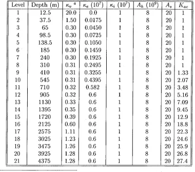
2.1 Ocean model vertical resolution and some physical parameters 17

3.1 Ocean spinup runs with different model configurations 35

3.2 Root-Mean-Square differences of the model T, S and o t from Levitus

(1994) climatology. 39

4.1 Standard deviations of annual and decadal mean SAT and SST for

some specified regions. 117

5.1 Rates of warming for three sub-layers in the TGM3 integration. . . . 148

6.1 Surface warming over the globe, hemispheres, land and oceans in

ATGM3 203

B.1 Salinity changes (psu) of the ocean interior observed in the ATGM3

(13)

List of Figures

2.1 Annual cycle of SST and SSS for relaxation data and model results

over North Atlantic and Southern Ocean 28

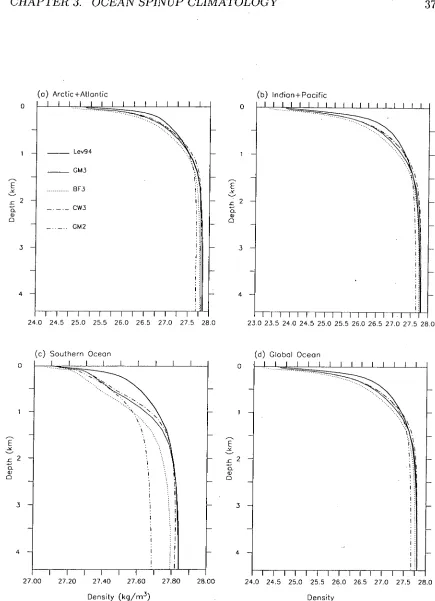
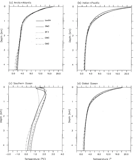
3.1 Vertical profiles of density (at) in the oceans. 37 3.2 Zonally averaged density (at) structure in the global ocean 3.3 Vertical profiles of temperature in the oceans 43

3.4 Zonally averaged global ocean temperature 45

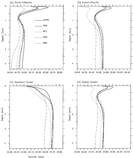
3.5 Vertical profiles of salinity in the oceans 47

3.6 Zonally averaged salinity in the global ocean 48

3.7 Surface heat fluxes from the GM3 solution and GM3 - GM2 51

3.8 Surface freshwater fluxes from the GM3 solution and GM3 - GM2. . 54

3.9 Surface buoyancy fluxes from the GM3 solution and GM3 - GM2. . 56

3.10 Northward heat and freshwater transports 58

3.11 Maximum depth of convection in the annual cycle. 61

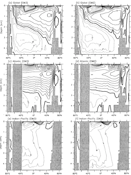
3.12 Meridional overturning streamfunctions. 65

3.13 Barotropic flow streamfunctions. 69

3.14 Horizontal currents at different levels in GM3 . 72

(14)

LIST OF FIGURES xiii

3.15 Difference of horizontal currents between GM3 and GM2 73

3.16 Annual mean windstresses from the NCEP and H-R climatologies. . 78

3.17 Wind-driven barotropic flow from the Sverdrup model. 81

3.18 Ekman pumping and the model vertical velocities at 25 m depth. . 83

4.1 Time series of global mean SST/SAT in control runs CGM3 and CGM2. 89

4.2 Changes of zonal mean SST in CGM3 and CGM2. 90

4.3 Geographical distributions of SST drift in CGM3 and CGM2 and the

SST difference between CGM3 and CGM2 93

4.4 Changes of zonally averaged SSS 94

4.5 Same as Fig.4.3 but for sea surface salinity. 95

4.6 Time series of sea ice area and volume in both hemispheres. 98

4.7 Differences of surface fluxes between CGM3 and CGM2. 99

4.8 Vertical profiles of density (at ), temperature and salinity. 101

4.9 Zonally averaged density (at ) structure for the global basin. 102

4.10 Same as 4.9 but for temperature. 103

4.11 Same as 4.9 but for salinity. 104

4.12 Time series of T/S changes for the entire ocean . 106

4.13 Overturning pattern for the last 50 year average. 108

4.14 Temporal variations of the NADWF and AABWF intensities. . . . 110

4.15 Barotropic streamfunction pattern for the last 50 year period. . . 111

(15)

LIST OF FIGURES xiv

5.1 CO2 forcing scenario (IPCC/IS92a) for the transient experiments

TGM3 and TGM2- . 119

5.2 Time series of SAT changes in TGM3 and TGM2 121

5.3 Geographical distributions of SAT changes 124

5.4 Time series of SST changes 126

5.5 Same as Fig.5.3 but for SST changes 128

5.6 Time series of sea ice area and volume 130

5.7 Changes of latitudinal distributions of surface heat fluxes over land

and the ocean in TGM3 131

5.8 Changes of sea surface heat flux and oceanic heat transport. 135

5.9 Evolution of zonally averaged decadal mean zonal windstress. 138

5.10 Evolution of zonally averaged P, E and runoff in TGM3. 138

5.11 Changes of sea surface freshwater flux in TGM3. 142

5.12 Time series of SSS changes from the TGM3 run 145

5.13 Changes of annual mean temperature in the global ocean interior. . 147

5.14 Zonally averaged global ocean temperature changes 150

5.15 Change of salinity in the global ocean interior 152

5.16 Changes of density (at ) in the global ocean interior 155

5.17 Thermal expansion induced global mean sea level change 157

5.18 Changes of overturning pattern in the global ocean 161

5.19 Same as 5.18 but for the Atlantic Ocean 162

(16)

LIST OF FIGURES xv

5.21 Time series of the NADWF and AABWF intensities. 165

5.22 Time series for changes in freshwater fluxes in the Southen Ocean and

the North Atlantic ₁₆₉

5.23 Time series for changes in annual mean SST and SSS over the Southen

Ocean and the North Atlantic 172

5.24 Time series for changes in annual mean SSD (at) over the Southern

Ocean and the North Atlantic 175

5.25 Changes of water column stratification in the Southern Ocean and

•the North Atlantic for TGM3 178

5.26 Barotropic streamfunction for year651-700 mean. 180

5.27 Changes of the major barotropic flows-ACC and others. 181

5.28 Average zonal wind and vertical structure of horizontal velocities in

the ACC zone 186

5.29 Evolution of the density structure across ACC 190

5.30 Changes of horizontal currents at different depths in TGM3 . 194

6.1 SAT changes in the accelerated integrations ATGM3 and ATGM2. . . 201

6.2 Time series of SST changes over the globe, SH and NH 202

6.3 Geographical distributions of SST changes 204

6.4 Changes of sea surface heat flux. 206

6.5 Evolution of northward heat transport 208

6.6 Evolution of zonally averaged annual mean zonal windstress 210

6.7 Latitudinal profiles of surface freshwater fluxes in ATGM3 211

(17)

LIST OF FIGURES xvi

6.9 Changes of temperature in the global ocean interior. 214

6.10 Zonal mean temperature changes in the global ocean interior. . 216

6.11 Changes of global ocean density (at) 217

6.12 Time series of the NADWF, AABWF and AABW outflow 220

6.13 Changes of the overturning pattern in ATGM3. 223

6.14 Time series of annual mean SSS, SST and SSD changes over the

Weddell and Ross Seas from the ATGM3 run 225

6.15 Evolution of the Southern Ocean Stratification in ATGM3 226

6.16 Time series of the ACC transport and the Gulf Stream 229

6.17 Time series of meridional density contrast across ACC. 230

6.18 Final state of the world ocean barotropic flow under 3x CO 2 condition

in the CSIRO model 231

A.1 Zonal mean surface heat and freshwater fluxes from AGCM and

OGCM-GM3 and adjustments for COGCM-GM3 and CGM2. 250

A.2 Zonal mean surface windstresses from the AGCM and the NCEP data

and the adjustments for CGM3 and CGM2. 253

A.3 Zonal mean SST and SSS adjustments for control runs 257

B.1 Changes of global ocean salinity and its effect on density. 259

B.2 Time series of salinity- and temperature-induced changes of stratifi-

cation in the Southern Ocean 263

B.3 Time series of global ocean THC in ATGM3 and ATGM3add 266

(18)

Chapter 1 Introduction

The Earth's climate changes. It is vastly different from what is was 100 million years ago when the high latitudes were heavily covered by tropical plants and most of the continents were playgrounds for the dinosaurs. During the last million years the Earth has experienced repeated extensive glaciation in the Northern Hemisphere (NH). Today's climate is largely different from what it was 18000 years ago when the last glaciation reached its peak and the NH was covered with much more ice sheets. Even over the past 2000 years the Earth has seen a variation in the global temperature up to 1 °C on either side of the present value. In the more recent past, say, since the late 19th century, the global average surface temperature has increased by 0.6±0.2 °C and it is very likely that the 1990s was the warmest decade and 1998 the warmest year in the instrumental record since 1861, as suggested by observations (IPCC 2001). Changes or variations of climate in the long history of the Earth have been largely attributable to the evolution of the Earth's geography, to fluctuations or periodicities in the Earth's orbit, and to long-term changes in the composition of the atmosphere.

In the future the global climate will surely continue to change. Apart from the natural causes, a new, external, driving force has been introduced since the Industrial

(19)

CHAPTER 1. INTRODUCTION 2

effect of their own activities on the climate since the early 19th century. By the

end of the 19th century and the early 20th century, it had been discovered that the amount of CO 2 in the atmosphere affected the global temperature through the greenhouse effect and that human activities were increasing the atmospheric CO 2 . Since the late 1960s, climate change induced by atmospheric CO 2 (which lately has been broadened to include the effect of other greenhouse gases and referred to as

equivalent CO 2 or simply CO2 ) has drawn more and more attention and has been

investigated extensively by various means. One of the many objectives of these

studies is to answer the question as to how and where the global climate evolves under the increasing CO2 condition. This is also the main target of the present study, which focuses on oceanic response to the long-term CO2 forcing.

1.1 Ocean Circulation and the Climate System

The world ocean covers 71% of the surface area of the globe. It is evidently the dominant primary source of water supplies for the Earth's ecosystem. Meanwhile, its huge amount of water mass makes it an immense reservoir of heat for the Earth's climate system. This heat storage capacity, working as a giant flywheel to the climate

system, acts to maintain, or say stabilize the state of the global climate: moderating

change but prolonging it once the change commences. Net thermal energy obtained by the ocean in tropical latitudes is transported to the polar latitudes, where part of

the heat is released back into the atmosphere and part is transported into the deep

ocean. In this process, ocean circulations, especially the meridional thermohaline

circulations (THC) play a crucial role.

The THC, driven by density differentials in the ocean, acts as a giant conveyer

belt (Broecker 1987, 1991), efficiently transporting heat and salt great distances

between basins and globally. In the Atlantic Ocean, the THC is manifested as warm,

saline surface water transported by the Gulf Stream and the North Atlantic current

(20)

temperature (SST) and sea surface salinity (SSS) in the northern North Atlantic are

considerably higher than that of the northern North Pacific at comparable latitudes

where no such strong THC is evident. When the high latitude North Atlantic saline

surface water cools, particularly in late winter, it becomes denser, destabilizing the

water column and triggering deep convection and hence the overturning. The sinking

branch of the overturning circulation brings the surface salty water into the deep layer of the occean, thereby producing the North Atlantic Deep Water (NADW).

This process is the so-called NADW formation (NADWF). The formed NADW can be carried (and distributed) by the southward return flow at depth to other places

and eventually penetrates the Southern Ocean until it is blocked by a zonal 'wall'

in the Circumpolar Ocean, i.e., the Antarctic Circumpolar Current (ACC). Only a minor part of this salty water can penetrate through the ACC and reach high latitude regions off Antarctica. Most of this water joins the ACC, flowing around Antarctica

and ventilating the Indian and Pacific Oceans, mainly through large-scale diffusion and meso-scale eddies. For compensation, upwelling occurs in the North Pacific, and a shallow return current is thus formed, which flows into the Indian Ocean

(through the Indonesian passages) and reaches the region off South Africa. There it joins the western boundary flow, i.e., the Agulhas Current. While most of the warm

water transported from the Indian Ocean is swept into the confluence of the ACC

and turns east, some is spun off into eddies that enter the Atlantic and then flows northwards into the North Atlantic. The above process roughly features a closed

large-scale meridional cell originating from the North Atlantic, which dominates the

world ocean meridional heat transport.

At the other side of the ACC, i.e., high latitude Southern Ocean off Antarctica,

an-other branch of the THC system is in operation. In the Weddell and Ross Seas, for

example, when sea ice forms or grows in winter, brine is rejected into the underlying

surface water, and the shallow water columns on the continental shelves lose

buoy-ancy so rapidly that they plummet to the bottom of the shelves and then keep sinking (along the continental rise) down the bottom of the ocean, forming the Antarctic

(21)

convection and overturning circulation off Antarctica, and the so formed AABW, which has the highest density in the world ocean (except for the Arctic Ocean), is spread northward by the deep meridional overturning cell and ventilates the bottom ocean of all basins with cold and relatively low salinity water.

(22)

and Keigwin 1987; Duplessy et al. 1988).

1.2 Stability of the Thermohaline Circulation

The above mentioned paleoclimatic evidence has raised the possibility of multiple equilibria of ocean circulation and rapid transition between different modes under certain external forcing, especially anomalies in the hydrological cycle over the North Atlantic. This, together with the importance of the THC in maintaining the global climate, has inspired a large number of studies on the stability of THC, in particular, the NADWF.

Most of these studies have been based on ocean-only models, with a focus on the sensitivity of NADWF to high latitude fresh water flux perturbations caused by local changes such as the Great Salinity Anomaly (GSA) 1 (e.g., Bryan 1986; Wright and Stocker 1991; Power et al. 1994; Rahmstorf and Willebrand 1995; Cai 1996b). However, results are highly model-dependent: the NADWF can be either extremely stable or very unstable. As can be understood, large uncertainty exists in the stand-alone ocean model results due in part to the lack of many important atmospheric feedbacks that operate in reality and strongly modify behaviours of the ocean.

To more realistically simulate the effects of high latitude freshening (either GSA-like events or variations in large scale atmospheric moisture transport) on the THC, cou-pled models of various complexity, from highly idealised atmosphere-ocean coucou-pled models (e.g., Nakamura et al. 1994; Saravanan and McWilliams 1995; Rahmstorf 1996; Wang et al. 1999) to comprehensive three dimensional fully coupled models (e.g., Manabe and Stouffer 1995; Cai et al. 1997), have been used such that feedback processes and interactions between the atmosphere and ocean are allowed. Although the results are diverse, the NADWF is found to be very sensitive to the imposed

(23)

freshening in most models. It can either be largely but temporally reduced or

com-pletely shut off and then recover, indicating the existence of multiple equilibria in

the model ocean. These results also provide some useful indications to the behaviour of world ocean under atmospheric CO 2 forcing which has been shown to enhance poleward transport of the atmospheric moisture and thus freshen the surface water

of high latitude oceans.

The past two decades have witnessed a growing concern about anthropogenic

influ-ence on the global climate. Thanks to the rapid advance in computing technology

and the development in human understanding of the climate system, coupled mod-els have become one of the most powerful tools for climate research and have been

widely used to study climate change induced by atmospheric greenhouse gas in-creases (e.g. Bryan et al. 1982; Spelman and Manabe 1984; Bryan and Spelman

1985; Bryan et al. 1988; Washington and Meehl 1989; Stouffer et al. 1989; Manabe et al. 1990, Manabe et al. 1991; Cubasch et al. 1992; Manabe and Stouffer 1993, 1994; Murphy and Mitchell 1995; Gordon and O'Farrell 1997; Hirst 1999;

Miko-lajewicz and Voss 2000), based on a variety of radiative forcing scenarios (IPCC 1990; IPCC 1996). Basically, these studies have been conducted to answer a pivotal question: how sensitive is the climate to the intensifying greenhouse effect? In other

words, how big is any pending climatic disruption likely to be? Although answers to these questions do not completely agree, all models show a commonality that

anthropogenic CO2 increase is changing the climate: it causes an increase in the surface temperature, at least in terms of the global average, i.e., global warming.

How does the ocean respond to the global warming? Most models simulate a

remark-able weakening, even complete shutoff of the NADWF under CO 2 increase forcing, although there are also models with a small change in the THC or even no response

of the NADWF intensity at all (e.g., Latif et al. 2000). Since the CO 2 increase is not expected to stop in the near future and its impact will be persistent and far-reaching,

a natural question, not only of scientific interest and importance, is therefore raised:

(24)

Due to the large time scale of the THC response to surface perturbations, to

an-swer these questions needs integrations extending over multi-centuries and millennia.

Such integrations (still) take a large amount of computational time. Therefore, only

a few studies have been carried out so far to investigate the long-term behaviour of

the world ocean THC under global warming using three dimensional fully coupled

models. One report on this, topic is by Manabe and Stouffer (1994) who observed the collapse of the NADWF in a CO2 quadrupling integration covering 500 years using the GFDL model. Lately, this integration had been extended to over 5000

years (Manabe and Stouffer 1999), and the NADWF is found to reintensify after year 900 of the simulation and fully recovers by year 1600, suggesting that the THC shutoff state is not a stable equilibrium in their model. More recently, Voss and Mikolajewicz (2001) found that, in their 850-year CO 2 quadrupling integration us-ing the ECHAM3/LSG model, the NADWF temporarily weakens by up to 50% at around year 140 (i.e., 20 years after CO2 quadrupling), and then slowly recovers, in contrast to the complete and lasting shutdown simulated in the GFDL model.

1.3 Southern Ocean and the Climate System

While most attention has been paid to the North Atlantic and the NADWF in

the above mentioned studies, Hirst (1999) carried out an integration covering 850 years using the CSIRO fully coupled climate model, with a transient increasing

CO2 followed by a three time CO2 stabilization forcing scenario, to examine the response of the Southern Ocean to global warming. He found that deep convection is

suppressed and the downwelling adjacent to Antarctica associated with the AABWF

nearly ceases by the time of CO 2 tripling. During the subsequent period of elevated stable CO2 , both the convection and AABWF do not recover at all. As a result, the water of the entire ocean below about 1.5 km depth remains relatively stagnant,

retaining a density which is too great to allow renewal from any source. The NADWF is found to be substantially reduced and become shallower in the first half of the

(25)

upper layers). These results are in contrast to the finding of Manabe and Stouffer (1994) that, under the four times CO2 condition in the GFDL model, the Antarctic overturning cell becomes weaker and shallower but never shuts off, whereas the NADWF collapses completely and stays inactive for a long time.

Although most previous studies, for some well-understood reasons, focus on the central role of the North Atlantic in climate change, all coupled global models suggest an important role for the Southern Ocean change in determining the global pattern of surface atmospheric response. It has been shown that changes in the Southern Ocean thermal advection and convection make the surface temperature there particularly resistant to the CO2 induced warming, contributing to a marked inter-hemispheric asymmetry in the pattern of global warming (e.g., Manabe et al. 1990, 1991; Manabe and Stouffer 1994; Murphy and Mitchell 1995). The commonly simulated feature that the NH as a whole warms much faster than the SH has significant potential consequences for regional climate change (e.g., Whetton et al. 1997).

(26)

Apart from affecting the carbon cycle, the Southern Ocean change has also potential impact on the ocean ecosystem. In the longer term, the possibility of deep ocean stagnation over many centuries raises the issue of development of extensive anoxia, with potential severe deleterious effects for marine biota. The associated changes in biological production may exert significant influence back on the climate system because the marine organisms, such as phytoplankton, are very important in the control of atmospheric CO2 via oceanic uptake. In particular, a reduced biological production leads to less consumption of CO₂ in the near surface waters, reducing air-sea gradients in CO2 content, hence lessening further sequestration of CO 2 in the ocean and increasing its build-up in the atmosphere. This feedback process is not included in the current generation of 'physical' models, but it does occur in reality

2• In any case, the Southern Ocean is an extremely important region for both the climate system and the ecosystem, especially in a long term view. Knowledge about the stability and change of the Antarctic overturning and the associated AABWF is critical for understanding the evolution of past climates and assessing possible climate changes in the future.

The Hirst (1999) integration highlights a possible long-term response of the ocean, especially the Southern Ocean, to the global warming forcing. However, the ongoing warming in the ocean interior indicates that the climate system is far from a final equilibrium state in the model. An important question for the long-term ventilation of the deep ocean is thus whether or not AABWF eventually resumes under stable elevated CO2 levels.

2Phytoplankton fix carbon from dissolved CO 2 through photosynthesis. When these organisms

(27)

1.4 Aims of This Study

This PhD program studies the response of the world ocean, in particular the South-ern Ocean, to CO2 induced global warming, making use of the CSIRO fully coupled climate model (mark2). An initial goal of this study was to modify the CSIRO OGCM in order to obtain an as realistic as practicable oceanic climate in terms of water properties, especially density structure in the Southern Ocean, for the use in coupled model climate research. This was partly motivated by the above men-tioned differences in response of the global THC to increasing CO₂ forcing between the CSIRO climate model and other models such as the GFDL model. Since the coupled ocean control climate of the CSIRO model used by Hirst et al. (2000) rep-resents a water stratification significantly weaker than in the observations (Levitus 1994), particularly in the high latitude Southern Ocean, due mainly to a low salinity bias in the deep oceans, it may be thought that the Southern Ocean overturning is unrealistically sensitive to the surface perturbation induced by CO 2 anomaly forc-ing. A reasonable speculation is that a more realistic representation of the world ocean stratification in the control run could lead to a weaker response of the THC to global warming forcing—for example, the AABWF may not shut off as quickly or completely or, if it does collapse, may recover sooner after CO ₂ stabilization.

(28)

features of the THC, and, naturally, a realistic representation of temperature and

salinity (and thus density) distributions in a prognostic ocean model is one of the

central indices for validating the performance of models. In this context, our result

with the new ocean formulation is to some extent more convincing, and allows the

small changes to the water masses which are already appearing in the observations

to be more clearly compared with the changes simulated by the model (Wong et al.

1999).

In general, the primary objectives of this PhD program include:

• to modify the CSIRO ocean model, with the aim of yielding a more realistic spinup climate than earlier versions in terms of water mass properties on basin to global scales for use in coupled model climate change studies;

• to initialise the ocean in the CSIRO climate model with the above obtained spinup solution and perform a long control integration to examine the stability of this new ocean climate;

• to carry out a long integration based on the above control run, with a tran-sient/stabilization CO 2 scenario to examine the expected more realistic' re-sponses of world ocean THC, especially the AABWF to global warming.

• to perform additional runs, accelerating the deep ocean convergence to

equi-librium, to examine the possible final state of the ocean in particular, under

stable elevated CO2 condition;

• to compare the behaviours of the ocean under CO 2 forcing in the new version model with that of an earlier version which has a quite different control climate

for the ocean, hence examining the dependence of ocean climatic responses to

(29)

1.5 Overview of This Thesis

Chapter 2 briefly introduces the CSIRO ocean model GM2 version from which this program is started. We have no intention of restating lengthy formulations such as the physical framework-the governing equations, numerical techniques and so on because this model is developed from the Cox-Bryan model and its basic configu-ration has been described in detail in a wide range of publications. In stead, some relevant details such as the surface conditions, (new) developments in the model parameterizations are discussed. However, the focus of this chapter is on the modi-fications of the surface thermohaline forcing fields. It is based mainly on the changes made in the surface forcing fields, together with the adjustments of some physical parameters, based on which the new version ocean model GM3 is formulated.

Chapter 3 documents the new ocean climate obtained using the GM3 version ocean model. Through comparison between the GM3 spinup solution, the GM2 climate and other spinup results achieved under different surface forcing conditions, success of the GM3 version in producing water properties closely matching the observations is highlighted. This comparison is presented in section 3.1. The following sections examine some other important elements of the ocean climate such as surface fluxes (section 3.3), meridional heat and freshwater transports, and the world ocean THC in particular (section 3.5.1). Also examined are the wind driven circulations (sec-tion 3.5.2). For this purpose, the Sverdrup model is used to estimate the wind driven depth-integrated flow. Comparison is made between this flow and the model simulated barotropic flow, and the difference is discussed. Further comparisons are made between the GM3 and GM2 versions in terms of the above important ther-modynamic and dynamic fields, aimed at revealing the respective advantages and weaknesses of these two versions in representing the ocean climate on basin and global scales.

(30)

extended further in this chapter between the coupled control climates. It is shown

that the noted differences or contrasts between GM3 and GM2 are generally well

maintained through the course of the two control integrations, both covering 800

years. Although both runs show very stable annual mean globally averaged climate, with negligible long-term trends in terms of all major quantities at the surface and in

the ocean interior, CGM3 is demonstrated to have a generally more realistic solution compared against the observations with results from other coarse resolution coupled

models. This strengthens our confidence in the performance of the new model when

used for climate change simulations. We note that appreciable regional drift can still exist, mainly in high latitudes such as the Arctic Ocean.

In Chapter 5 we represent the results of a global warming experiment TGM3. This run is initialized with the control (CGM3) solution at the end of model year 100, and subsequently is forced by an increasing (equivalent) CO 2 level according to the IPCC/IS92a radiative forcing scenario for greenhouse gases for the period 1880-2082. By model year 302 (calendar year 2082), CO2 concentration is triple the control level, and TGM3 is continued thereafter for another 1100 years with the CO 2 concentration held constant at this elevated level (referred to as 3 x CO 2 ). Also presented are the results from a parallel run TGM2 which is initialized from CGM2 and employs an

identical CO2 scenario, but with a shorter stabilization duration (650 years). The

TGM3 integration may be taken as an extension of Hirst (1999) (which may be referred to as TGM1) except for the use of the 'updated' ocean component (with

a more realistic spinup climate in the Southern Ocean in particular, as repeatedly

addressed) and some refinements to the ice model which can better represent the

sea ice-ocean interaction process. The gradual reintensification of NADWF and the

complete shutoff of AABWF noted in TGM1 are still evident in both the TGM3 and TGM2 runs. Moreover, the shutoff state of AABWF in TGM3 lasts through

the whole period of the 1100 year 3 x CO 2 stabilization with no sign of returning, and the associated deep overturning cell dies away, leaving a isolated bottom ocean

with no ventilation. Details of other oceanic responses, both at the surface (i.e.,

(31)

CHAPTER I. INTRODUCTION 14

(i.e., temperature, salinity, density, and horizontal currents), are documented, and relevant mechanisms for these changes are examined. Differences in changes between TGM3 and TGM2 are noted and discussed.

Chapter 6 presents results of two additional runs AGM3 and AGM2. These runs stem from the TGM3 and TGM2 (i.e., initialized with the state from the end of year 700), respectively, and make use of the Bryan (1984) technique to accelerate the deep ocean convergence to equilibrium. We show that, under acceleration, the deep ocean warms more rapidly than the upper water in due course. After 230 years accelerated integration (equivalent to 6300 years for the deepest ocean), the Southern Ocean water column becomes destabilized to such an extent that deep convection is reactivated and the AABWF is able to operate again, and thereafter the whole climate system evolves into a new, quasi-stable state. This is the case for both runs. To examine if this state is the same as what can be expected from the normal time-stepping integration, further extensions to these accelerated runs are conducted and made to continue for 500 years with the acceleration switched off. We show that the accelerated solution does need some time with normal time-stepping running to adjust and finally settle down to a more stable but slightly different state. Reasons of the resumption of AABWF is discussed in detail.

Finally, chapter 7 presents the overall conclusions of this study. Major achievements are highlighted and further discussed. Also included in this chapter are remarks on some possible caveats for the model (and simulations) and the potential resultant uncertainties.

(32)

Chapter 2 The CSIRO Ocean Model

2.1 General Description

The CSIRO global ocean general circulation model is a coarse resolution, gridpoint, z-coordinate model. It is developed from the Cox (1984) code for the primitive equation general circulation model of Bryan (1969) and is described in detail by Moore and Reason (1993) and Moore and Gordon (1994). For the version as a component of the CSIRO coupled model (mark2), the model domain consists of a global coverage of the world ocean and the horizontal grid has a resolution of 5.625° longitude by about 3.2° latitude, corresponding to the R21 Gaussian grid of the spectral atmospheric GCM.

(33)

CHAPTER 2. THE CSIRO OCEAN MODEL 16

and the Greenland-Scotland sill (800 m). Several inland seas (Baltic Sea, Black Sea, Caspian Sea) included in the model are not linked to the world ocean and act on the world ocean only via affecting the heat flux adjustment when coupled to the atmospheric model. Due to the coarse resolution of the model, the Mediterranean Sea, Hudson Bay and the Persian Gulf are also not linked directly to the world oceans but the effect of water exchange between these water bodies and the world ocean is parameterized via a mixing of tracers between the closest adjacent grid points across the unresolved straits. For example, the rate of exchange between the Mediterranean Sea and the North Atlantic is calculated assuming a total volume transports of 0.8 Sv, with outmixing depth assumed to be 800 m for the Gibraltar Strait, whilst the other unresolved straits have smaller exchange rates and shallower outmixing depths. Drake Passage extends from 65°S to 56°S in the model (com-pared to the actual width from 63°S to 57°S) so as to accommodate three velocity grid boxes.

This model prognoses potential temperature, salinity, the two horizontal velocity components, and diagnoses the vertical velocity by using the continuity equation. At the sea surface, the rigid-lid approximation is employed and the bottom is assumed to be insulating. No-slip and insulating conditions are applied at lateral boundaries. The flow variables are Fourier filtered in the northern high latitude (north of 74.9°N) for the purpose of relaxing the severe time step restriction associated with advective numerical stability due to the convergence of meridians toward the North Pole. No filtering is applied in the Southern Oceans.

(34)

[image:34.553.88.468.170.505.2]

Table 2.1: Ocean model physical parameters (in units of cm2s-1): vertical diffusivity kV)

isopycnal thickness diffusivity ic e , isopycnal tracer diffusivity kz , lateral viscosity Ah, and vertical viscosity A. Note the last column gives accelerating scales (dimensionless) used in Chapter 6 for speeding up the ocean convergence.

Level Depth (m) ic.„ a Ke (107) ni (107) _{Ah (1P) Av} Kac

1 12.5 20.0 0.0 00 ₀₀

0 0 00 0 0 GO 00 00 00 c0 00 (X ) 00 00 0 0 0 0 00 0 0 00 0 0 0 0

20 1

2 37.5 1.50 0.0175 20 1

3 65 0.30 0.0450 20 1

4 98.5 0.30 0.0725 ' 20 1 5 138.5 0.30 0.1050 20 1

6 185 0.30 0.1459 20 1

7 240 0.30 0.1925 20 1

8 310 0.31 0.2495 20 1

9 410 0.31 0.3255 20 1.33

10 545 0.31 0.4395 20 2.07

11 710 0.32 0.582 20 3.48

12 905 0.32 0.6 20 5.16

13 1130 0.33 0.6 20 7.09

14 1395 0.35 0.6 20 9.45

15 1720 0.39 0.6 20 12.9

16 2125 0.60 0.6 20 18.8

17 2575 1.11 0.6 20 22.3

18 3025 1.23 0.6 20 24.6

19 3475 1.26 0.6 20 25.9

20 3925 1.28 0.6 20 26.8

21 4375 1.28 0.6 20 27.4

a Value at level k should be understood as between level k and level k+1.

profile has the weakness that it does not respond to the potential influence of local

physical factors such as the stability on the diffusivity. Some studies have employed

a scheme that relates the vertical diffusivity to the Brunt-Vaisala frequency

(buoy-ancy frequency) N by setting ic, to be proportional to the inverse of N (e.g, Gargett 1984; Mourn and Osborn 1986; Kraus 1990; Hirst and Cai 1994, Hirst et al. 2000).

However, this scheme is still not well physically validated and Hirst and Cai (1994)

found little change in the resulting ocean solution. Thus, the N-1 dependence of vertical diffusivity is switched off in this study and instead the Bryan and Lewis

(35)

model. Convective mixing in this model is simulated by setting an enhanced local vertical diffusivity value of 10 6 cm2s' in regions of static instability, whenever di-agnosed during the integration, letting temperature and salinity be mixed vertically over the unstable portion of the water column. In this adjustment process heat and salt are conserved by mixing adjacent unstable levels completely. Although some researchers (e.g., Marotzke 1991) reported that the parameterization for convection is important to the thermohaline circulation, we do not include such a scheme in our model as per England (1993), who used a model similar to ours and found little adjustment of the model solutions from the switch in convection schemes.

The Cox (1987) scheme for isopycnal tracer diffusion is incorporated, via the small angle approximation to the Redi (1982) diffusion tensor, to represent more realis-tically the tendency for heat and salt to be mixed on surfaces of constant density. We set the isopyncal diffusivity ki to be spatially uniform with the value of 1 x10 7

cm2s -1 although some other researchers (e.g., England 1993) adopt a depth depen-dent isopycnal diffusivity in their models. This parameterization is discussed further in the following section.

This model version employs the Gent and McWilliams (1990) scheme for eddy-induced advection, which is also discussed in more detail in the following section. The isopycnal thickness diffusivity n e is set to be 0.6x10 7 cm2s -1 below 800 m, above which it decreases linearly to zero at the surface as required by the continuity constraint imposed on the eddy-induced transport. This is in contrast to that of GM2 and an earlier version (Hirst et al. 2000, referred to as GM1) where Ice is set to

be lx 107 cm2s' below 270 m. In addition, a weak and depth-dependent background horizontal diffusivity is used to replace the isopycnal thickness diffusivity in the high northern latitude region (beginning from 74.9°N) to avoid spurious temperatures and salinities.

(36)

2.2 Parameterizations

It is widely accepted that rapid tracer diffusive mixing in the real ocean occurs pri-marily along neutral surfaces (locally referenced constant potential density surfaces, McDougall 1987) which are generally not horizontal, and this is referred to as isopy-cnal mixing. In contrast, mixing across the neutral surfaces is believed to be weak in the real ocean (McDougall and Church 1986). The prescribed large horizontal diffu-sivity, which used to be commonly employed in ocean models for numerical reasons, may cause unrealistically strong diapycnal mixing, especially in regions of steeply sloping neutral surfaces, thus resulting in serious distortion of the solution for both eddy-permitting and coarse-resolution models (Cummins et al. 1990; Hirst et al. 1996). To parameterize the oceanic tracer transport by mesoscale eddies and elimi-nate, or at least reduce the effects of the above spurious horizontal diffusive fluxes, two more physically based schemes have been employed in the CSIRO OGCM, as has also been done in many other models around the world.

(37)

with this scheme still suffer deficiencies such as unrealistically weak stratification at high southern latitudes, which leads to extensive deep convection and large flux adjustment needed to damp the climate drift when coupled to an atmospheric model, which potentially distorts the global warming pattern in transient experiments for climate change induced by green-house gases. The version of CSIRO OGCM with both isopycnal mixing and the artificial horizontal background diffusivity (Gordon and O'Farrell 1997) is referred to as version HB.

A more recent development which helps to overcome the above problem of spurious diapycnal mixing is the implementation of the Gent and McWilliams scheme (Gent and McWilliams 1990; Gent et al. 1995, hereafter referred to as the GM scheme), which parameterizes the adiabatic transport of oceanic tracers by mesoscale eddies. The GM scheme expresses the additional eddy-induced advection as a function of the resolved density and has an effect on the large-scale density field like diffusion of neutral density thickness along the neutral surfaces (Gent et al. 1995). This scheme is physically based and acts on an OGCM akin to imposing a very large vertical viscosity, and therefore allows for substantial reduction or complete elimi-nation of the unphysical large horizontal diffusivity in the model used for numerical purposes. Many researchers (e.g., Danabasoglu and McWilliams 1995; Duffy et al. 1995; Boning et al. 1995; England 1995; Robitaille and Weaver 1995; Hirst and Mc-Dougall 1996) have implemented GM schemes in their OGCMs and show that their Cox-Bryan-Code based z-coordinate OGCMs can be run with a realistic dianeutral mixing rate, without the prescribed high horizontal diffusivity.

With the GM scheme, eddy-induced horizontal transport velocity is diagnosed and added to the usual resolved-scale (referred to as "large-scale" or "Eulerian-mean") horizontal velocity to give the "effective transport velocity" (Gent et al. 1995; Hirst and McDougall 1996; Hirst et al. 2000). The vertical component of either the eddy-induced transport or the effective transport velocity is obtained using the continuity equation.

(38)

provements upon the implementation of GM scheme in their OGCM. The major achievements include generally smaller and less noisy surface fluxes near Antarctica, more realistic deep water properties and a substantial reduction of deep convection near Antarctica, which, in the version with fictitious horizontal diffusivity, seriously depletes the salinity of Circumpolar Deep Water (CDW), leading to marked salinity deficiencies in the deep Indian and Pacific Oceans, and severely distorting the sur-face flux patterns near the Antarctic as mentioned above. The GM scheme also has a substantial effect on model dynamics. Hirst and McDougall (1998) showed that the meridional overturning circulation, when viewed in density coordinates, changes remarkably upon the implementation of the GM scheme, e.g., the evident residual Deacon cell in the earlier versions like HB, which is induced by the horizontal diffu-sivity, disappears completely and the separate direct Antarctic and deep circulation cells in the HB model are fully merged in the GM version. This solution is believed to represent the real ocean better than that of the HB version, and is also in broadly better agreement with that of the eddy-permitting FRAM Southern Ocean model (Doos and Webb 1994; McIntosh and McDougall 1996).

Moreover, Hirst et al. (1996) and Hirst et al. (2000) examined the performance of the GM scheme in the ocean under coupled conditions. Their experiments demonstrated that the beneficial effects of the GM scheme mentioned above are all generally well maintained during the coupled integration and these improvements are especially pronounced in the high latitude Southern Ocean. In addition, the coupled model with the GM version ocean (referred to as the GM version coupled model) requires smaller surface flux adjustments and displays markedly reduced climate drift in comparison to the earlier HB version ocean as reported by Gordon and O'Farrell (1997).

(39)

tation of ocean circulations and tracer distributions. One of the initial goals of this study is to obtain an oceanic climate which is as realistic as possible, using the above described state-of-the-art OGCM with proper surface boundary conditions, and to incorporate it in the CSIRO coupled model for the purpose of climate change simulations and sensitivity experiments.

2.3 Surface Boundary Conditions

The most traditional and still commonly used boundary condition for the OGCM is relaxation forcing for the model surface tracers, that is, the surface tempera-ture and salinity values are restored towards observed climatology via a Newtonian damping law, with a constant timescale ranging from days to months. The implied effective surface fluxes of heat and salinity/freshwater can then be diagnosed via the restoration, and the specified tracer climatologies, or say the apparent salinities and temperatures (Haney 1971), which vary temporally and spatially, are often de-signed to give observed surface fluxes when surface tracer values match observations (Han 1984). This technique was firstly used for surface thermal forcing based on the justification of Haney (1971) that there is direct feedback between the oceanic surface temperature and the air temperature above the sea surface, and it allows for large-scale thermal coupling of the ocean and atmosphere. However, its use in forc-ing the model surface salinity is not physically justified because the freshwater flux, which is determined from precipitation and evaporation (i.e., P - E), is essentially independent of the surface salinity.

A kind of mixed boundary condition is sometimes used in ocean modelling studies.

Such forcing keeps the temperature restoring but replaces the unphysical salinity

(40)

dependent behaviours in the ocean, including the polar halocline catastrophe (Bryan 1986), low-frequency oscillations (Marotzke 1989) and decadal timescale oscillations (Weaver and Sarachik 1991a,b; Cai 1995). Moreover, under such mixed boundary conditions, the model solution is very sensitive to the surface freshwater forcing magnitude, and the model solution can either be unstable or reach multiple equilib-ria. So, although it may be a useful approach to investigate ocean response to the change in the hydrological cycle of the atmosphere, mixed boundary conditions are not suitable for ocean spinup integrations that aim to obtain a stable and realistic ocean equilibrium for the coupled model.

Another type of forcing for surface tracers is the flux boundary condition, which specifies the net heat and freshwater fluxes over the whole model domain. The heat flux can be specified in the way that derives the freshwater flux, i.e., it can be either the observed climatology or simply diagnosed from an initial ocean spinup with re-laxation forcing. Furthermore, both the heat and freshwater fluxes can be specified via the product of an atmospheric GCM. This is of particular interest for climate change experiments using an atmosphere-ocean coupled model. If the pre-coupling ocean spinup, driven by the AGCM implied fluxes, can reach a reasonable equi-librium, flux adjustments, which are widely used to damp the climate drift upon coupling, will naturally vanish. Unfortunately, the ocean model tends to behave erratically under fixed flux forcing, with the SST evolving far from the observed surface temperature (e.g., Rosati and Miyakoda 1988). This drift in SST occurs because the specified fluxes may have large errors or uncertainties due to the limi-tations in observations and because the air-sea feedback which operates under the Haney (1971) thermal forcing is switched off under the fixed flux forcing.

(41)

and freshwater fluxes are not linked via evaporation process as they are in reality. Barnier et al. (1995) designed standard bulk formulas to configure OGCM thermal boundary conditions, which express the net heat flux as a function of SST, with the climatologies of SST and net heat flux calculated using the European Center for Medium-Range Weather Forecasts (ECMWF) analyses. Large et al. (1997) employ bulk forcing in the NCAR OGCM, utilizing the evolving model SST and monthly atmospheric fields based on both the reanalyses of the National Center for Environmental Prediction (NCEP) and satellite data products. It needs to be mentioned that for the OGCMs that are not coupled to an explicit sea ice model, such as the NCAR model and CSIRO model, bulk forcing is used only for open (ice free) sea water and a strong restoring in temperature and salinity is still needed under sea ice. In addition, a weak salinity relaxation is also applied to open water for the purpose of damping the potential instability which would otherwise occur. Large et al. (1997) found that, compared to relaxation forcing, bulk forcing produces poleward heat and salt transports in better agreement with most oceanographic estimates and maintains the abyssal tracer distributions closer to observations.

(42)

the model surface temperature towards needs to be mentioned. Firstly, although it

may seem a more natural choice, the Levitus SST and SSS together do not supply our model with a proper surface relaxation forcing under which formation of realistic

water masses can be simulated. Previous studies (e.g., Hirst and Cai 1994) reveal

serious inconsistencies between the Levitus values and some other observations. For

example, the Levitus values at 10 m depth (which dominates in the interpolation

to the top level of our model) give a peak winter density remarkably lower than

that of observations in many important water mass formation regions such as the Labrador Sea and Norwegian/Iceland/Greenland Sea (and in some regions the

sur-face density is even higher than that at 10 m depth). We found that the combination of Levitus SSS and BMO SST gives a generally better density field, especially for the winter density peak greater than 28.0 kg m -3 which is featured in the Norwe-gian/Iceland/Greenland Sea and close to that of observations (Rudels et al 1989; Clarke et al. 1990). Secondly, the BMO SST is used for the CSIRO AGCM spinup

and thus is a natural choice for the ocean spinup, considering the compatibility between these two components for the CSIRO coupled model.

The dynamic boundary condition for our model is configured with the climatology of atmosphere to ocean momentum flux (windstress). Contrasting many earlier

studies (e.g., Gordon and O'Farrell 1997; Hirst et al. 1996, Hirst et al. 2000) where Hellerman and Rosenstein (1983) windstress monthly climatology (referred to as

H-R wind data hereinafter) is used, this study employs the windstress climatology determined from the NCEP 1951-1990 monthly mean and interpolated onto the

model grid points. Compared to the H-R wind which is too strong over tropical

oceans and too weak over the Southern Ocean especially near Antarctica, the NCEP

windstress is believed to be more realistic in terms of the general distribution pattern

and magnitude, especially in the near Antarctica region. In addition, the NCEP

climatology is closer to the CSIRO AGCM windstress than the H-R data. So its

use in our model will reduce the required momentum flux adjustment for coupling, and help in diminishing the possible impact of change in windstress upon coupling

(43)

using different windstress forcing data in the spinups will be described briefly in next chapter.

2.4 Modification of the Surface Forcing Fields

Trial experiments showed that, under the (original) BMO SST and Levitus SSS forc-ing, our model still fails to produce realistic world ocean water mass properties and thermohaline circulations. Although the relaxation tracers indicate a high enough winter peak density that generally matches observations as mentioned above, the restored model upper-level tracers can only give a peak density of 27.90 kg m -3 in the Norwegian/Greenland Sea, and a peak value of 27.5 kg m -3 in the Labrador Sea, both are much lower than the observed counterparts, i.e., over 28.0 and 27.78 kg m', respectively. This inconsistency in the North Atlantic is hypothesized to be one of the main factors causing the weak deep convection and thus too shallow penetration of North Atlantic overturning. To test this hypothesis, we make some further adjustments to the forcing, aimed at obtaining more realistic model upper-level temperature and salinity fields (and therefore better surface density features). Obviously this pursuit also favours our endeavour to provide a reasonably realistic simulated SST for the coupled model in climate studies.

It is well known that the model SST and SSS simulated under relaxation forcing always suffer a more or less "shift" from the climatological values, especially the peak and trough values. This is due partly to the mixing between neighbouring grid points with different properties, and partly to surface fluxes lagging observations caused by the unreality of a posteriori restoring the model surface tracers to the

observed, both depending on the relaxation timescale. It is from this deviation that

(44)

to the atmosphere and is therefore taken as inappropriate for our purposes. The alternative method used to reduce this departure, in particular the SST anomaly, is to adjust the forcing fields so as to tie the resultant model surface solution close to observations. We choose to adjust the surface forcing fields, instead of using too short relaxation timescales, for our ocean spinup integration, in such a way that the mean computed surface value at a point corresponds to the corresponding mean observed value. In principle, this is equivalent to imposing a time centered restoration rather than a time lagged restoration.

A series of short time integrations are performed to modify the thermal forcing field, using an intermediate relaxation time scale of 20 days. Firstly a short run is conducted under the original BMO SST climatology forcing and the model SST anomaly is diagnosed, i.e., BMO SST minus model top level temperature in our case. This anomaly is then imposed on the old forcing field for the subsequent short run, from which a new SST anomaly can be obtained and used to modify the forcing values again. Repeat this precess a few times until a model SST field closest to the original BMO climatology is reached. The final forcing field is what we need for the long term ocean spinup to be coupled to the atmosphere. We initially employed the above modification to the SST forcing globally and found the adjustment is very large and noisy in the middle latitudes and equatorial regions, and results in unreasonably large and noisy heat fluxes there. So we constrain the modification to within the high latitudes in both hemispheres (north of 40°N and south of 60°S) where the deep water masses are formed, with the change in forcing values at the demarcation smoothed. In addition to the above adjustment, the BMO SST dataset is also carefully tuned 0.5 - 2.0 °C higher in the North Sea to reduce the false high density center there which appears when forced under the original BMO SST data and may lead to spurious water mass formation at that location.

(45)

0 (a) NA ( 0 °W-40°E, 5 —8 °N) (b) 0 out of 0°S

0.8 0.4 0.0

_GM3 SST _ .New BMO SST

_..GM2 SST _ Old BMO SST -0.4

F- t')

-0.8

-1.2

Y

(d) Ross Sea (SW corner

GM3 SSS - . New Levitus SST - . GM2 SST _.._. Old Levitus SST

yJ J I AgSpO t NvDc

[image:45.554.68.498.106.323.2]

SSS ( 35 + 0. 01x )p su SSS ( 34 + 0. 01x )p su 80. 70. 60. 50. 40. 30. 20.

Figure 2.1: Annual cycle of SST and SSS for relaxation data and model results over the North Atlantic (NA) and Southern Ocean (S0)/southwestern corner of the Ross Sea.

and GM3, respectively. The lag of the model SST to the surface forcing is evident. The annual cycle of the final forcing SST is substantially modified and so is the resulting model temperature. In the North Atlantic, if we neglect the impacts from other factors, such as the salinity forcing change and the slight differences of model physics between GM2 and GM3, the cooling by 2 °C of the forcing can lead to a decrease of 0.95 °C in the model temperature in March, and 1.7 °C warming in August making the model temperature 0.8 °C higher in September. The overall improvement in model temperature in the North Atlantic is achieved at the cost of larger heat fluxes in that region, as indicated by the larger temperature difference, and clearly, with such an adjustment, we still see too high model (GM3) winter temperature compared to the original BMO SST, due mainly to the freezing point constraint for the relaxation SST. A similar situation occurs in the Southern Ocean where the modified model winter temperature is significantly cooled but is still not cold enough. This shows the limitations of the above modification schemes to the SST, which is a characteristic of sea ice freezing regions.

(46)

resentation of the model surface density distributions. However, the abovedescribed method for SST forcing adjustment is found unsuitable for the SSS forcing because it causes a very noisy freshwater flux distribution over the global ocean. We thus con-strain the modification to within the North Atlantic region and some grid points near Antarctica, with the principle that the resulting model SSS distributions in these regions capture both the temporal and geographical characteristics of the Levitus SSS climatology. In the North Atlantic (20-70°N, 20-90°W), the adjustment made to the Levitus SSS ranges from -0.78 to 0.85 psu in the annual cycle. Significant changes are made in high latitudes, with the largest enhancement (0.5 psu in late winter and 0.85 in early summer) employed at a point (50.6°W, 55.7°N) in the cen-tral Labrador Seas and the largest reduction (0.78 psu for all seasons) imposed on a point (61.9°W, 58.9°N) near the mouth of Hudson Strait. In the southeastern Greenland coastal region the Levitus SSS is also subject to a reduction from 0.2-0.5 psu year round. In lower latitudes, modification is weak (0.1-0.2 psu) but extensive so as to yield a realistic winter salinity distribution there. The overall change in the Levitus SSS forcing in the North Atlantic is about 0.1 psu enhancement year round, as displayed by Fig.2.1c, making the model surface about 0.1 psu saltier as well. Such changes made to restoration SSS and SST do result in reasonable model water properties near the surface, and more importantly, keep the model winter peak density close to observations in the NADWF regions and consequently result in a stronger and deeper overturning circulation there compared to solutions under other surface forcing conditions.

Transient and long term behaviour of the world ocean under global warming