Computer simulation and investigation of underwater two part and multi tow systems

Computer Simulation and Investigation of Underwater Two-Part

and Multi Tow Systems

S '-'--

p

(i

Susantha D Ranmuthugala

(:0..J l_l a. -..d.. 1--u d o · .Lr "'' Q

.:c: ('

Submitted in fulfilment of the requirements for the degree of

Doctor of Philosophy in Engineering

University of Tasmania

This thesis contains no material which has been accepted for a degree or diploma by

the University or any other institution, except by way of background information and

This thesis may be made available for loan and limjted copying in accordance with the

Copyright Act 1968.

Note:

ABSTRACT

To maximise effectiveness, towed underwater sonar bodies generally require

perturbations from the steady state motion to be minimised. The instantaneous position of the towed body is influenced by the unsteady, wave-induced motion of the

surface vessel, transmitted via the tow cable. This can render the trajectory of the underwater body beyond acceptable limits for sonar operations.

In an effort to decouple this motion, a two-part tow configuration has been employed.

This thesis describes a three-dimensional dynamic computer model developed to

investigate two-part tows by modelling the individual cabl~s separately and coupling

them dynamically. This approach also enables the modelling of series and parallel

multiple tow configurations. The cable system, modelled using a three

degree-of-freedom finite difference approach, is then coupled to the ·six degree-of-degree-of-freedom

underwater towed bodies at the appropriate locations of the cable system. The

modelling of the cable as a continuous medium and the derivation of the stress wave

speeds are also presented, followed by the validity and.effects of representing it as a

discretised model.

The solution to the dynamic equations describing the motion of the discretised tow

configuration is carried out using an implicit multi-step numerical technique, subject

to specific boundary conditions. This allows the values to be improved through an

iterative procedure, until sufficient convergence is achieved.

An introduction into the use of such numerical techniques in engineering and an

analysis of the numerical procedure used in the solution are also presented. The

requirements for accuracy and numerical stability of the integration technique are

investigated and a guide to the time interval for the time ·stepping algorithm is

deduced.

The computer model is successfully validated using experimental results from scaled

model tests in a circulating water channel. These results together with those obtained

from full scale sonar trials utilising small coastal craft are used to further investigate the behaviour of the two-part tow configuration to varying parameters. The

The thesis also presents a detailed review of the various methods available to

investigate underwater cables and vehicles, together with prediction methods for their

hydrodynamic coefficients. The latter coefficients for the scaled models used in the project are obtained via experimental procedures.

Although a number of investigations have been carried out dealing with aspects of

underwater towing operations, the strength of this investigation lies in that it combines

these aspects, i.e._ mathematical modelling, computer simulation, prediction of the

hydrodynamic coefficients, scaled model experiments, full scale trials, and the

ACKNOWLEDGEMENTS

I wish to thank the following for their assistance and valuable contribution during the

project.

My supervisors Professor Michael Davis from the University of Tasmania and Dr Stan

Gottschalk from AMC for their guidance, support, and encouragement. Dr

Gottschalk's ability to make sense of my somewhat disorganised draft material at such

short notice, and return them with in-depth comments and recommendations has been

a major factor in the completion of this project.

Mr Brendon Anderson and Mr Garry Campanella from DSTO for their assistance in organising the experimental work and providing the ever important industry input.

Special mention must be made of Mr Anderson for his patience, encouragement, and for reminding me on numerous occasions that timeframes are not infinitely

expandable.

Robert Evans from AMC, Peter Graham, Greg Wright, Darryl Gaston, and Darius

Juchnevicius from DSTO, Tim Mak from AMECRC and a number of staff members

from AMC and DSTO for their assistance in the experimental stages of the project.

Ross Warden from DSTO for assistance in video recording the scaled model tests and

their subsequent analysis. Dr Ian MacGillivray from DSTO for assisting with

analysing experimental data.

Special thanks to Dr Paul McShane, Dr Colin Buxton, and Mr Ian Cartwright, my line managers during the project, for their support and understanding that enabled me to

complete the work. My colleagues at AMC for their encouragement, even if only to

ask "when will you ever finish?".

AMC, DSTO, and AMECRC for their assistance, including financial and in-kind

contributions, throughout the project.

Finally my wife Preeni for putting up with a short tempered husband who spent all his

spare time staring at a computer screen, not to mention the mountain of paper that

defied all her efforts at cleaning, my paren13for all their support during the project, and

my two children who made a supreme effort to stay out of Dad's path and expressed

everyone's relief at the end of the project by stating "Dad can now stop playing with

TABLE OF CONTENTS

Abstract

Acknowledgements

List of Illustrations

List of Tables

Nomenclature

Abbreviations

Equation Numbering Scheme

Chapter 1 Introduction

1.1 Definition of Problem

1.2 Outline of Thesis 1.3 Tow Configuration

1.4 Static and Quasi-Static Cable Models

1.5 Dynamic Cable Models

1.6 Tow Cable I Fish Models · 1.7 Solution Techniques

1.8 Underwater Vehicle Models

1.9 Experimental Investigation and Validation

Chapter 2

Modelling Techniques

2.1 Introduction

2.2 Dynamic Cable Models

2.2.1 The Method of Characteristics

2.2.2 Finite Difference Method

2.2.3 Hinged Rod Method 2.2.4 Finite Element Method

2.2.5 Lumped-Mass Method

2.3 Cable Drag and Inertia Forces

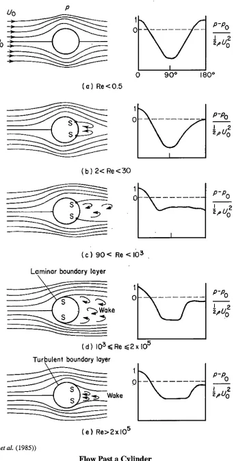
2.3.1 Flow Past a Smooth Long Rigid Cylinder

2.3.2 Effects on Drag Coefficient due to Surface

62

63

Roughness and Turbulence 70

2.3.3 Drag on a Rigid Cylinder Inclined to the Flow 71

2.3.4 Morison's Equation 74

2.3.5 Hydrodynamic Cylinder Coefficients in Harmonic

Flow 76

2.3.6 Vortex Induced Hydrodynamic Forces 83

2.3.7 Hydrodynamic Coefficients Selected 91

2.4 Towed Fish Models 91

2.5 Towed Fish Hydrodynamic and Acceleration Coefficients 93

Chapter 3

2.5.1 Towed Fish Acceleration Coefficients

2.5.2 Towed Fish Static and Dynamic Hydrodynamic

Coefficients

Cable and Fish Model

3.1 Modelling of the System

3.2 Axes System

3.2.1 Cable System Transformation Matrix

3.2.2 Tow Fish Transformation Matrix

3.3 Cable Model

3.3.1 Drag Force

3.4 Equations of Motion for Cable Nodes

3.4.1 Junction

3.4.2 Boundary Nodes

3.5 Tow Fish Model

Chapter 4

3.5.1 Force Equations for Tow Fish

3.5.2 Moment Equations for Tow Fish

3 .5 .3 Linearisation of Equations

3.5.4 Equations of Motion for Tow Fish

Solution Algorithm and Program Outputs

4.1 Overview

4.2 Quasi-Static Model

4.3 Dynamic Model Solution Algorithm 150

4.3.1 Boundary Nodes 154

4.3.2 Junction 155

4.3.3 Matrix Solution 157

4.3.4 Angular Displacement of Tow Fish 161

4.3.5 Solution Procedure 162

4.4 Program Outputs 164

4.5 Multiple Tows in Series 167

4.6 Multiple Tows in Parallel 173

ChauterS

Analysis of the Numerical Method 177

5.1 Introduction 177

5.1.1 Derivation of the Houbolt Scheme 181

5.2 Comparison between the Lumped Mass Model and the

Continuous Cable Model 185

5.2.1 Continuous Cable Model 185

5.2.2 Wave Speeds 192

5.2.3 Relationship between Continuous and Discrete

Systems 192

5.2.4 Effects due to Discretisation 197

5.3 Stability and Accuracy 200

5.4 von Neumann (Fourier) and Routh-Hurwitz Methods 202

5.4.1 von Neumann (Fourier) Method 203

5.4.2 Routh-Hurwitz Method 204

5.5 Matrix Stability Method 205

5.5.1 Modal Superposition 205

5.5.2 Stability Analysis 209

5.5.3 Stability of the Houbolt Integration Scheme 212

5.5.4 Non-linear Systems 215

5.6 Accuracy 217

5.6.1 Accuracy Analysis of the Houbolt Scheme 220

5.7 Natural Frequencies of the Model 226

Chapter 6

Experimental Methods and Validation

6.1 Introduction

6.2 Scaled Model Trials

6.2.1 Scaled Model Trial Configurations 6.3 Scaled Model Test Results

6.3.1 Response of the Two-Part Tow due to Vertical

236

236 236

238 240

Excitation 241

6.3.2 Response of the Two-Part Tow due to Horizontal

Excitation 253

6.3.3 Conclusion from the Scaled Model Trial Results 260

6.4 Full Scale Trials 261

6.4.1 Full Scale Trial Results 263

6.5 Scaled Model Hydrodynamic Coefficients 267

6.6 Valid~tion of the Computer Program 269

Chapter7 Conclusion

7.1 Summary

7 .2 Conclusions and Recommendations

7 .3 Future Work

Bibliography

Appendix A

Experimental Results

AppendixB

Computer Program Flowcharts

List of Program Flowcharts

275

275

279

281

283

299

331

LIST OF ILLUSTRATIONS

Figure

1.1 Tow Configurations (a) to (i) 1.2 Two-Part Tow

L3 Conventional Tow

1.4 Typical Transfer Function for Shallow and Deep Water Mooring

Cases

2.1 Cartesian Coordinates of Cable

2.2 Continuous C~ble Element

2.3 t-s Solution Mesh

2.4 Hinged Rod Segment

2.5 Finite Element Model

2.6 Equivalent Nodal Forces on Finite Element

2.7 Tension Forces in Finite Element

2.8 Lumped Mass Model

2.9 Flow Past a Cylinder (a) to (e)

Page No.

2 and3 4 7 12 34 34 39 46 53 54 55 61 67

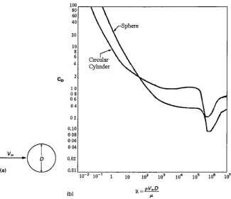
2.10 _Drag Coefficient for Cylinders and Spheres 68

. .

2.11 Typical Variation of Dra9 Coefficient with Reynolds Number for a

Smooth Cylinder 68

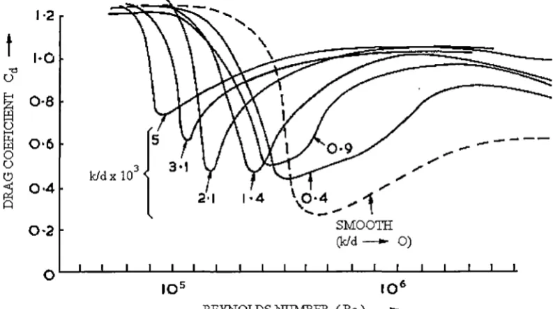
2.12 The Drag of Sand Roughened Cylinders 71

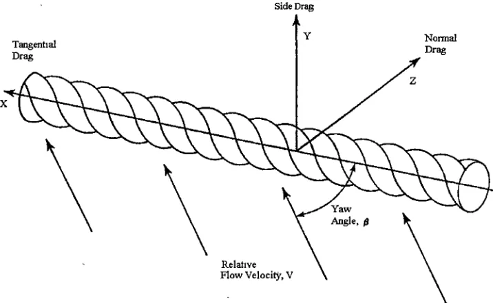
2.13 Direction of Drag Forces on a Cable in a 3D Flow Field 72

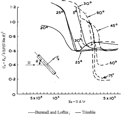
2.14 Variation. of Drag Coefficient for Inclined, Smooth Cylinder~ 73

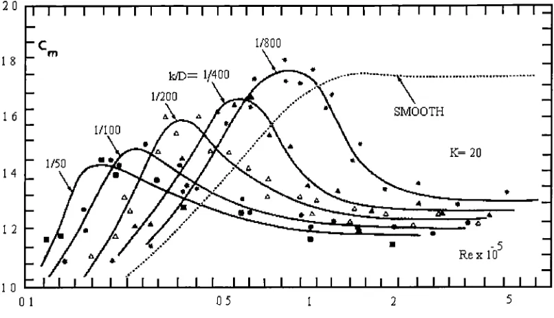
2.15 Drag Coefficient versus Reynolds Number for KC

=

Various Values of Relative Roughness 79

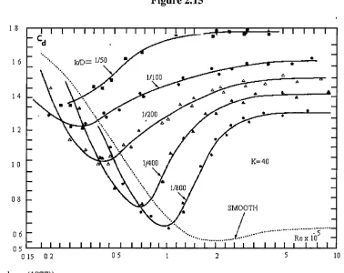
2.16 Drag Coefficient versus Reynolds Numbe~ for KC

-=

Various Values of Relative Roughness · 79

2.17 Inertia Coefficient . versus Reynolds Number for KC = 20 and for ·

Various Values of Relative Roughness

·so

2.18 ln~rtia Coefficient versus Reynolds Nm?b~r for KC-= 40 and for

Various Values of Relative Roughness 80

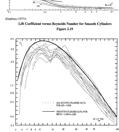
2.19 Lift Coefficient versus Reynolds Number for Smooth Cylinders 81

2.20 Lift Coefficient versus KC for a Relative Roughness of 1/200 81

2.21 Effective Lift Coefficient during Vortex Shedding against Effective

2.22 Drag Coefficient Amplification during Vortex Shedding against Wake

Response Parameter 87

2.23 Drag Coefficient during Vortex Shedding against Reduced Velocity 88

2.24 Orientation of an Underwater Vehicle 94

3.1 Coordinate Transformation for Cable 106

3.2 Right Hand Coordinate System for Towed Fish 106

3.3 Coordinate Transformation for Towed Fish 108

3.4 Lumped Mass Model of the Two-Part Tow 109

3.5 Cable Node "i" 110

3.6 Cable Junction Node "j" 119

3.7 Boundary Nodes 121

(a) Towed Fish, (b) Depressor, (c) Surface Vessel

3.8 Three-Dimensional Towed Fish 124

3.9 Geometry of the Towed Fish 124

3.10 Rotation of Unit Vectors of Towed Fish 127

(a) Rotation about X Axis, (b) Rotation about Y Axis

(c) Rotation about Z Axis

3.11 Forces and Moments at Tow Point (1) and Centre of Gravity (G) of

Towed Fish 131

4.1 Two-Part Tow Modelled with a Single Cable 144

4.2 Two-Part Tow Modelled with Two Cables 144

4.3 Multiple Tow in Series Modelled with a Single Cable 145

4.4 Multiple Tow in Series Modelled with Separate Cable Systems 145

4.5 Quasi-Static Fish Model 147

4.6 Conventional Tow - Surge 165

4.7 Two-Part Tow 1 - Surge 165

4.8 Conventional Tow - Heave 165

4.9 Two-Part Tow 1 - Heave 165

4.10 Conventional Tow - Pitch Angle 165

4.11 Two-Part Tow 1-Pitch Angle 165

4.12 Change in Pitch Angle with Location of Junction 166

4.13 Two-Part Tow 1 - Path of Vehicles 167

4.14 Two-Part Tow 1 - Depth 167

4.15 Two-Part Tow 1 - Pitch Angle 167

4.16 Multiple Tow Fish in Series 168

4.18 Series Multi-Tow - Path-Fast

4.19 Series Multi-Tow - Path - Fast- Slow

4.20 Series Multi-Tow - Depth-Fast

4.21 Series Multi-Tow -Depth- Slow 4.22 Series Multi-Tow - Pitch Angle -Fast

4.23 Series Multi-Tow - Pitch Angle - Slow

4.24 Difference Curve - X Direction 4.25 Difference Curve - Y Direction

4.26 Difference Curve - Depth

4.27 Difference Curve - Pitch Angle

4.28 Multiple Tow Fish in Parallel

4.29 Parallel Multi-Tow -Path

4.30 Parallel Multi-Tow -Depth

4.31 Parallel Multi-Tow - Pitch Angle

5.1 Spectral Radius of Numerical Integration Schemes with Zero

171 171 171 171 171 171 172 172 172 172 173 176 176 176

Damping 215

5.2 Amplitude Decay and Period Elongation 219

5.3 Amplitude Decay and Period Elongation of Numerical Integration

Schemes 219

6.1 Circulating Water Channel 237

6.2 Top View of Channel 237

6.3 Experimental Procedure 237

6.4 Scaled Models 237

6.5 Recording of Vertical Motion 240

6.6 Recording of Horizontal Motion 240

6.7 Surface Excitation Mechanism 240

6.8 Depressor and Towed Fish Response for Configurations Cl

i

6.9 Depressor and Towed Fish Response for Configurations C21 to C23 243

6.10 Depressor and Towed Fish Response for Configurations C31 to C33 243

6.11 Depressor and Towed Fish Response for Configurations B3 l to B33 243

6.12 Depressor and Towed Fish Response for Configurations A31 to A33 243

6.13 Depressor and Towed Fish Response for Configurations 121to123 245

6.14 Depressor and Towed Fish Response for Configurations 131 to 133 245 6.15 Depressor and Towed Fish Response for Configurations H31 to H33 245

6.18 Depressor and Towed Fish Response for Configurations E31 to E33 247

6.19 Depressor and Towed Fish Response for Configurations H31 to H33 247

6.20 Depressor and Towed Fish Response for Configurations K31 to K33 247

6.21 Depressor and Towed Fish Response for Configurations C21 to C23 249

6.22 Depressor and Towed Fish Response for Configurations X21 to X23 249

6.23 Depressor and Towed Fish Response for Configurations F21 to F23 249

6.24 Depressor and Towed Fish Response for Configurations T21 to T23 249

6.25 Depressor and Towed Fish Response for Configurations 121 to I23 249

6.26 Depressor and Towed Fish Response for Configurations AH21 to

AH23 249

6.27 Depressor and Towed Fish Response for Configurations C31 to C33 251

6.28 Depressor and Towed Fish Response for Configurations AA62 to

AA64 251

6.29 Depressor and Towed Fish Response for Configurations AA42 to

AA44 252

6.30 Depressor and Towed Fish Response for Configurations AB42 to

AB44 252

6.31 Depressor and Towed Fish Response for Configurations J31 to J33 252

6.32 Depressor and Towed Fish Response for Configurations AC22 to

AC24 252

6.33 Depressor and Towed Fish Response for Configurations AD22 to

AD24 252

6.34 Towed Fish Response for Configurations YY21 to YY23 253

6.35 Towed Fish Response for Configurations YAl l to YA14 253

6.36 Towed Fish Response for Configurations YA21 to YA24 253

6.37 Towed Fish Response for Configurations WA21 to W A23 253

6.38 Towed Fish Response for Configurations YD21 to YD23 255

6.39 Towed Fish Response for Configurations YG21 to YG23 255

6.40 Towed Fish Response_ for Configurations YC21 to YC23 255

6.41 Towed Fish Response for Configurations WC21 to WC24 255

6.42 Towed Fish Response for Configurations W A21 to W A23 255

6.43 Towed Fish Response for Configurations WB21 to WB24 255

6.44 Towed Fish Response for Configurations YA21 to Y A24 257.

6.45 Towed Fish Response for Configurations YB21 to YB23 257

6.46 Towed Fish Response for Configurations W A21 to W A23 257

6.47 Towed Fish Response for Configurations WD21 to WD24 257

6.48 Towed Fish Response for Configurations YD21 to YD23 258

6.50 Towed Fish Response for Configurations YG21 to YG23 259

6.51 Towed Fish Response for Configurations YE21 to YE23 259

6.52 Towed Fish Response for Configurations YF21 to YF23 259

6.53 Towed Fish Response for Configurations WA21 to W A23 259

6.54 Towed Fish Response for Configurations WE21 to WE24 259

6.55 Towed Fish Response for Configurations WF21 to WF24 259

6.56 Full Scale Trial Single Part Tow 261

6.57 Full Scale Trial Two-Part Tow 261

6.58 Aft Deck of Deploying Vessel 261

6.59 Deploying of Two-Part Tow 261

6.60 Use of HPMM to obtain the Hydrodynamic Coefficients 267

6.61 Coefficients for Tow Fish 268

6.62 Vertical Coefficients for Depressor 268

6.63 Horizontal Coefficients for Depressor 268

6.64 Pitch Angle of Tow Fish for 131 - Computer - Degrees 270

6.65 Pitch Angle of Tow Fish for 131 - Experiment - Degrees 270

6.66 Heave of Tow Fish for 131 - Computer - Centimetres 271

6.67 Heave of Tow Fish for 131 - Experiment - Centimetres 271

6.68 Surge of Tow Fish for 131 - Computer - Centimetres 271

6.69 Surge of Tow Fish for 131-Experiment- Centimetres 271

6.70 Tension at Surface for 131- Computer- Kilograms 271

6.71 Tension at Surface for 131 - Experimental - Kilograms 271

6.72 Pitch Angle of Tow Fish and Depressor for C31 Computer

-Degrees 272

6.73 Pitch Angle of Tow Fish and Depressor for C31 Experiment

-Degrees 272

6.74 Heave of Tow Fish and Depressor for C31 - Computer - Centimetres 272

6.75 Heave of Tow Fish and Depressor for C31 Experiment

-Centimetres 272

6.76 Surge of Tow Fish for C31 - Computer - Centimetres 272

6.77 Surge of Tow Fish for C31 - Computer - Centimetres 272

6.78 Tension at Surface for C31 - Computer - Kilograms 273

6.79 Tension at Surface for C31 - Experimental - Kilograms 273

6.80 Yaw Angle of Tow Fish for Y A22 - Computer - Degrees 273

6.81 Yaw Angle of Tow Fish for Y A22 - Experiment - Degrees 273

6.82 Sway of Tow Fish for Y A22 - Computer - Centimetres 273

LIST OF TABLES

Table

4.1 Conventional and Two-Part Tow Configuration Information

4.2 Series Multi-Tow Configuration Information

4.3 Parallel Multi-Tow Configuration Information

6.1 Full Scale Trail - Limiting Parameters

6.2 Trial 1 - Summary of Results

6.3 Trial 2 - Summary of Results

6.4 Tow Configuration Information for Validation Runs

6.5 Statistical Analysis of the Computer and Experimental Results

Al Scaled Model Tests AMC - Information

A2 Scaled Model Tests AMC - Results

A3 Trial 1 - Tow Information

A4 Trial 2 - Tow Information

A5 Trial 1 - Tow Results

A6 Trial 2 - Tow Results

A7 Trial 2 - Results - Direction to Swell

A8 Trial 2 - Results - Cable Length

A9 Trial 2 - Results - Tow Velocity

AlO Trial 2 - Results - Depressor Wing

All Trial 2 - Results - Types of Tows

A list of Flowcharts in Appendix B is given at the beginning of the

Appendix

Page No.

164

170

175

262

264

264

270

274

299

304

309

311

313

317

320

322

324

327

329

NOMENCLATURE

The following defines the major symbols used in this thesis. Since the work m this

thesis encompasses the fluid mechanics and solid mechanics disciplines, some

symbols traditionally have more than one meaning. In order to maintain consistency

throughout the thesis, the symbols selected reflect those used by other authors in this

field. Some variables and constants are defined at the relevant locations in the text.

General Convention

SI units are implicit.

For a dummy variable "A":

A A [A] A A ,... A vector A matrix A matrix A

derivative of A with respect to time

second derivative of A with respect to time

unit vector A

Variables and Constants

A

A,A,A

Ai

Amm

Amu

Amrx· ,y' ,z' Am

Alx',y',z'

Aab

Afab

cross sectional area

vectors representing the body rotational angles and their derivatives

cross sectional area of cable segment "i"

normal added mass coefficient of cable segment "i"

tangential added mass coefficient of cable segment "i"

added mass of the towed fish in the X', Y', and Z' directions hydrodynamic inertia (added mass) matrix of cable element

added inertia of the towed fish about the X', Y', and Z' axes

where a

=

=

mass matrix terms of the manipulated equation of motion of the fish

as defined in equations (3.97)

where a

=

=

mass matrix terms of the equation of motion of the fish as defined in

Ap

Au,Bu

[A]T

[Ar'

B21, B23

Ca

cd

Cm

en

Cw

cross sectional area of the fish perpendicular to the X axis

geometrical area of the body, (usually the cross-sectional area to the

flow or the surface area)

projected area of cylinder in the plane perpendicular to the direction of flow

amplification matrix

matrices defined in equations (2.9), (2.17), and (5.46)

transpose of matrix [A]

inverse of matrix [A]

variables defined in equations (3.96)

added mass coefficient

drag coefficient

equivalent drag coefficient

linearised equivalent damping coefficient in equation (2.77)

hydrodynamic coefficient

lift coefficient

inertia coefficient

cable drag coefficient in the normal direction

cable drag coefficient in the tangential direction

wave speed

trigonometric terms defined in equations (3.29)

where b

=

extra terms of the constraint equation for the junction in comparison

to the standard constraint equ~tion (4.18), defined in equations (4.31)

and (4.47)

where t = 0, 1, 2, 3, 4, ...

constants defined in equations (5.11) and (5.20) damping matrix

diameter

diameter of cable segment "i"

variable defined in equation (3.23)

modulus of elasticity

partial differential terms as defined in equations (4.19) to (4.21) error in the cable segment length "i", between the span of the nodal

F, f

F1x,y,z

Fct1x,y,z

Fct1x',y',z'

Fe1x,y,z

p. _IOX,y,z

Fr

Ff,x' ,y' ,z'

p' fx' ,y' ,z'

Fftx',y'z'

f

f n

G

Gu, Hu

G(U)

g

I, J, K1,K2

lax',y',z'

lx',y',z'

A A A

i, j, k

J k k =E k =G

[E1F1G1CD] converted to a true tri-diagonal matrix, as defined in

equation (4.35)

force vectors

forces on node "i" in the X,Y, and Z directions

drag forces (global) on segment "i" in the X, Y, and Z directions

drag forces (local) on segment "i" in the X', Y', and Z' directions

mean drag force in equation (2. 77)

any additional forces on node "i" in the X, Y, and Z directions

represents all forces except tension forces, acting on node "i" force vector acting on the fish

components of

Fr

summed forces in the equation of motion of the fish, defined in

equations (3.84) and (3.85)

summed forces in the manipulated equations of motion of the fish,

defined in equations (3.98)

hydrodynamic force, i.e. drag, lift, or side force

measured force

tension vector along element "i" as defined in equation (2.49) and

(2.52)

frequency

natural frequency

centre of gravity of towed fish

variables defined in equations (2.21) vectors defined in equations (2.23)

acceleration due to gravity (9.81 m/s2)

variables defined in equations (3.18)

moments of inertia of the towed fish at the centre of gravity about the

X', Y', and Z' axes, respectively

moments of inertia of the towed fish at the tow point about the X', Y',

and Z' axes, respectively

unit vectors along u, v, and w (local) axes system

Jordan form of Ap, with eigenvalues O"pi) of Ap along its leading

diagonal. stiffness matrix

cable element elastic stiffness matrix

cable element geometric stiffness matrix

kt

kw

L,M,N1,N2

Lllt(R N ~t) Lp

mab

m· e1x,y,z

MrGx' ,y' ,z'

Mfx',y',z'

M' fx' ,y' ,z'

Pnx,y,z

p, q, r

p,q,

t

p

p = I

Pab

tangential stiffness of a single lumped mass

wave number

Keulegan-Carpenter number

variables defined in equations (3.25)

local truncation error of the integration scheme

load operator

length of cable segment "i"

length of fish

length of the smallest element in the lumped mass model

wavelength

mass terms mass matrix

mass of node "i", ie. the addition of half the mass of each adjacent

segments

where a

=

=

mass matrix terms

mass and added mass of any additional weight attached to node "i"

mass of towed fish

cable mass per unit length

moment vector

moment vector acting on the fish, about its centre of gravity

components of Mta about the X', Y', and Z' (local) axes moment vector acting on the fish, about its tow point

components of Mn about the X', Y', and Z' (local) axes

summed moments in the equation of motion of the fish, defined in

equations (3.84) and (3.85)

where a= x, y, z

variables defined in equations (3.29a)

variables defined in equations (3.32)

angular velocity components (roll, pitch, and yaw) of the fish about

the X', Y', and Z' axes

angular acceleration components of the fish about the X', Y', and Z'

axes

matrix of eigenvectors of Ap

tensor defined in equations (2.39) and (2.40)

where a

=

=

p(Ap) spectral radius of the amplification matrix ( Ap)

distance from the tow point (1) to the centre of gravity (G)

R, R, R displacement, velocity, and acceleration vectors

Re Reynolds number

Rm, Rm, Rm modal displacement, velocity, and acceleration vectors

ri cable element mass ratio defined in equations (2.~9) and (2.40)

s arc length of any point along the cable

Str Strauhal number

T tension of cable

Ti tension of cable segme~t "i"

T₁ tentative tension of cable segment "i"

Tr tension of cable segment attached to towed fish

Trx,y,z component of the cable tension in the X, Y, and Z (global) directions

Trx',y',z' component of the cable tension in the X', Y', and Z' (local) directions

A

t unit vector in cable element direction from bottom to top

t time

tn,mm minimum natural period of the cable mesh

tn,a natural period of "a" mode

tp period of the cycle

U vector defined in equations (2.9), (2.17), and (5.46)

U₀ velocity vector of the towc;d fish at its centre of gravity (G)

u, v, w

u, v, w

v

v

Ynx,y,z

acceleration vector of the towed fish at its centre of gravity (G)

velocity vector of the towed fish at its tow point

acceleration vector of the towed fish at its tow point

local velocity components along the local (X', Y', and Z') axes

system

local acceleration components along the local axes .system

velocity

velocity vector

water current velocities along the X,Y, and Z directions

maximum velocity

reduced velocity

relative velocity between the body and the surrounding fluid relative velocity vector

time dependent relative velocity

velocities (global) of node "i" relative to the water in the X, Y, and Z

VSrix,y,z

VSnx' ,y' ,z'

WR X,Y,Z x,y,z

x,y,z

x,y,z

x', y', z'

Xa, Ya,Za

Ym

YRMS

velocities (global) of cable segment "i" relative to the water in the X,

Y, and Z directions

velocities (local) of cable segment "i" relative to the water in the X',

Y', and Z' directions

net weight of node "i" in water, i.e. the addition of half the net weight

of each adjacent segments

wake response parameter

global axis system as defined in sub-section 3.2

displacement along the X, Y and Z directions velocities in the X, Y, and Z directions

acceleration in the X, Y, and Z directions

local axes system as defined in sub-section 3.2

displacement of node along the X', Y' and Z' directions

components of the distance (RG) from the tow point (1) to the centre

of gravity (G), measured from the tow point and positive in the

directions of the local axes system

cross flow displacement amplitude

root mean square anti-nodal displacement

Greek Symbols

a, ~.y

~f <I> \jf p Pc O' E /.., /.., Awi AwL AwT !

right hand rotation of the fish about the Y (pitch), X (roll), and Z

(yaw) axes

where i

=

parameters of multi-step integration algorithm, (see equation (5.4))

frequency parameter defined by equation (2.86)

horizontal angle of the cable with the X axis

vertical angle of the cable with the X-Y plane

density of the water in which the towing occurs

density of cable

stress in cable or cable element when stretched

local strain in cable or cable element when stretched eigenvalues

matrix that_ stores the eigenvalues along its main diagonal

where i = 1,2,3,4,5,6

wave propagation speed along a continuous cable system longitudinal wave speed along a continuous cable system

K

u

(l)

Q

<pa

where i = 1,2,3, ... ,n

eigenvalues of Ap

visco-elastic damping coefficient

coefficient to allow for hysteresis

angular velocity vector of cable element

natural frequency

angular velocity vector of the towed fish having components a,

J3,

y

mass per unit length of the cable

mass of the displaced water per unit length of the element

variable to solve the tri-diagonal matrix [EiF,Gi] recursively, as

defined in equations (4.38) and (4.39)

where a= 1, 2

characteristic lines associated with Aa, defined in' equations (2.13),

shape function of cable element

variable length along the element divided by the element length, (s/li)

damping ratio

Cos-1 ~

C0₀ (-Cosv ±iSinv)

r+o

cable system transformation matrix

tow fish transformation matrix

modal transformation matrix defined in equation (5.88)

time step (increment)

represents the change in a parameter

error

or

amplitude error, which increases the damping by a small quantity 8a

phase error, which increases the frequency of oscillation by a small

quantity 8a/2n. Kronecker delta,

tension correction term of cable segment "i"

variables defined in equation (2.80)

eigenvectors

matrix that stores the eigenvectors along its columns

Subscripts

D

e

f

G

i+l/2

i-112

j

n

u, v, w

x,y,z

t

0

1

Supercripts

k

m

t

0

(1)

(2)

depressor

additional forces or weights

towed fish

centre of gravity of tow fish

ith cable node, (or i1h cable segment located between nodes "i" and

"i+ 1 ")

cable element just after node "i"

cable element just prior to node "i"

cable node representing the junction

cable node representing the surface towing vessel

direction along axes of local coordinate system

direction along X, Y and Z axes

time

centroid of tow fish

tow point on tow fish

iteration index

convergence correction superscript in equation (4.7)

time

equilibrium position (configuration)

top of cable rod element

ABBREVIATIONS

2D

3D

AMC

AMECRC

DOF

DSTO

FDM

FEM

HPMM

LMM

RAN

ROV

two dimensional

three dimensional

Australian Maritime College

Australian Maritime Engineering Cooperative Research Centre

degree of freedom

Defence, Science and Technology Organisation

finite difference method

finite element method

horizontal planar-motion-mechanism

lumped mass method

Royal Australian Navy

Remotely Operated Vehicle

EQUATION NUMBERING SCHEME

All equations are numbered aligned to the relevant chapter and in ascending order

through that chapter. For example equations in Chapter 3 will commence from (3.1)

and continue as (3.2), (3.3) and onwards.

When an equation number represents a set of equations, the number is usually

sub-divided, e.g. equations (3.8a), (3.8b), and (3.8c). When referring to such a set of

equations, if all of the equations in that set are being addressed, then they will be

referred to as equations (3.8). However, if only some of the equations from the set

CHAPTERl

INTRODUCTION

1.1 Definition of Problem

A sonar platform is an example of a submerged body that is towed behind a surface

vessel. Such platforms are used extensively in offshore, military, hydrography, and

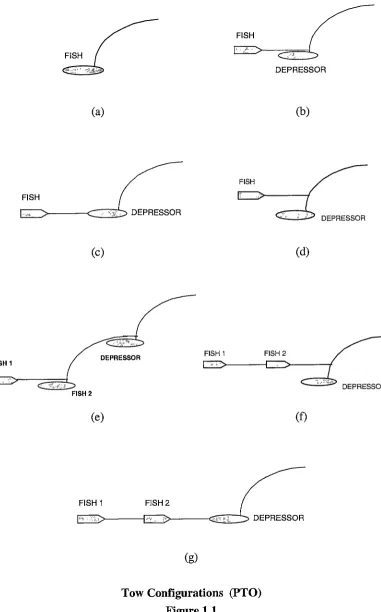
oceanography activities, (see Figure 1.1). They generally require that perturbations

from the steady state motion are minimised in order to ensure clear sonar imaging.

The instantaneous position of the submerged towed object (referred to as the "fish" in

this text), is influenced by the relative motion between the cable and the water, the

hydrodynamic characteristics of the fish, and the unsteady wave induced motion of the

surface vessel.. Depending on the sea state and the towing vessel's response to it, the

wave induced motion can be sufficiently large to render the trajectory of the tow fish

beyond acceptable limits for sonar operations. This motion is transmitted to the fish

along the tow cable.

The Royal Australian Navy (RAN) uses towed sonar vehicles for a variety of

operations. One task is the deployment of side scan sonar from small vessels to detect

mines in coastal waters. As the operation is in coastal (shallow) waters, the length of

the tow cable can be relatively short, e.g. 25 metres. In addition, the relatively small

size of the surface vessel can lead to large wave induced motions. These conditions

can adversely affect the motion of the sonar vehicle, resulting in imperfect sonar

operations.

The wave induced motion of a towed body attached to a conventional tow system used

by the RAN, exceeds the acceptable motion rates in the six-degrees of freedom by

more than 60%, (see Tables 6.2 and 6.3 in Chapter 6). In order to reduce this motion,

and thus improve the efficiency of sonar operations, the Defence, Science and

Technology Organisation (DSTO) of Australia was tasked with optimising the tow configuration. The investigation was carried out by the Australian Maritime College

(AMC), DSTO, and the University of Tasmania with assistance form the Australian

FISH

FISH

DEPRESSOR

(a) (b)

FISH

(c) (d)

DEPRESSOR FISH 1 FISH 2

(e) (f)

FISH 1 FISH 2

j;>-~~-<ZeI[:'.:::: DEPRESSOR

(g)

Tow Configurations (PTO) Figure 1.1

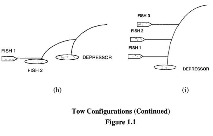
FISH 1

FISH2

(h)

FISH 3

DEPRESSOR

Tow Configurations (Continued) Figure 1.1

DEPRESSOR

(i)

Since the surface vessel's motion is usually beyond the control of the operator, the

transmission of the wave induced motion of the surface vessel to the towed fish can be

reduced by:

• designing the fish to be more hydrodynamically stable;

• incorporating adaptive control surfaces on the fish; and/or

• decoupling the surface vessel motion from the fish.

This investigation centres around the third option, since it is an effective, cost efficient

method of achieving the required objective.

Various methods have been employed in tow configurations to increase decoupling of ·

the motions. One such method is the two-part tow shown in Figure 1.2. It consists of

a primary cable attached at its top end to the surface vessel (i.e. the vessel towing the

sonar), while the bottom end is attached to a depressor. The latter ensures that the tow

configuration maintains the required depth. The fish is attached to the lower end of

the primary cable by a secondary cable. The point of attachment (referred to as the

"junction") can be varied along the cable length, thus influencing the behaviour of the

towed fish. The two-part tow configuration and its behaviour are explained in Asplin

In order to investigate and optimise the tow configuration, the project was carried out

in three stages:

1. the development of a three-dimensional (3D) dynamic computer model incorporating the decoupling effect, to predict the motion of the fish due to the excitation at the surface;

2. scaled model tests of the tow configuration; and

3. full scale trials.

TRAIL

PRIMARY GABL'

SECONDARY CABLE

I

TOWED FISH

JUNCTION

DEPRESSOR

Two-Part Tow Figure 1.2

DEPTH

The computer model of the two-part tow incorporates tow line and fish dynamics as

well as the decoupling effect of the two separate lines. The response envelop of the

configuration can be determined by varying the parameters of the model. This allows

the configuration to be optimised to give an acceptable trajectory for the tow fish.

Since the attachment point between the two cables can be varied along the length of

the primary cable, it is inadequate to model the tow configuration as a single cable system, with an "extra" lumped mass representing the depressor. One must model the

two cables separately and then dynamically couple them at the junction. Following a

comprehensive review of the literature, the author was unable to find any

This concept allows the investigation of not only varying points of attachment, but

also multiple towed bodies, i.e. more than one secondary cable attached at various

points along the primary cable, (see Figure 1.l(i))

The results from the computer model were validated and supplemented using:

• experimental data from scaled model tests of the two-part tow configuration

conducted in the circulating water channel at the Australian Maritime College in

Launceston; and

• full scale trials at Jervis Bay and Port Phillip Bay.

1.2 Outline of Thesis

The remainder of this chapter outlines the tow configurations investigated and reviews

the literature relevant to the modelling of such systems. This review includes static,

quasi-static and dynamic cable modelling techniques, current underwater tow models,

numencal procedures employed to solve cable I tow models, and the modelling of underwater vehicle. Finally the experimental investigation is introduced. The rest of

the chapters are structured as follows.

Chapter 2 looks at the methods available to investigate cable and underwater bodies.

It first looks at the more popular mathematical representations of dynamic cable

modelling and the time domain solution techniques utilised. The selected method for

this study is justified based on the ability and suitability of the various methods. The

prediction of drag and inertia coefficients of cables is yet a highly researched area.

Chapter 2 details some of the investigations, analyses the behaviour of the fluid flow

around the cable, and presents current methods used to predict the relevant

coefficients. Finally the modelling techniques available for underwater vehicles and

the prediction of the relevant coefficients are discussed.

In Chapter 3, the mathematical modelling of the quasi-static and dynamic two-part

and multi tow configurations is detailed. This includes the modelling approach used

for the cable junction, series and parallel multiple tows, and the integration of the tow

I depressor fish into the cable model. This is followed by the numerical solution procedure in Chapter 4, where the numerical integration scheme and the required

required to deal with the two types of multiple tow configurations. Typical results for

the various configurations are also presented.

Chapter 5 analyses the numerical procedure used in the solution, and includes an

introduction into such numerical techniques in engineering. The modelling of the cable as a continuous medium and the derivation of the stress wave speeds are

presented, followed by the validity and effects of representing it as a discretised

model. The stability and accuracy of the numerical procedure utilised is analysed and

the prediction of a suitable time step to meet these criteria is discussed.

Chapter 6 details the scaled model experiments and the full scale trials, and analyses

the results in order to investigate the behaviour of the two-part tow. The scaled model

test results are also used to validate the computer model, which includes the

experimental calculation of the hydrodynamic coefficients of the scaled models.

Finally Chapter 7 presents the conclusions and recommendations.

Appendix A gives the results from the scaled model tests and the full scale trials,

while Appendix B presents detailed flowcharts of the computer model.

1.3 Tow Configuration

Conventional towing arrangements consist of a tow cable attached at its upper end to

the surface towing vessel and its lower end to the fish, (Figure 1.3). This

configuration leads to large coupling effects, thus giving unacceptable fish motion due

to the transmission of the excitation at the cable's upper end down to the fish. The

two-part tow, shown in Figure 1.2, consists of a primary cable towed from the surface

vessel in a similar manner to the conventional tow, except that the fish is replaced by a

depressor to maintain the required depth of the cable's configuration. The fish is then

attached to the depressor (Figure l.l(c)) or to the lower end of the primary cable

(Figure 1.l(d)) by a secondary cable.

Usually the primary cable is negatively buoyant, while the towed fish and the

secondary cable are neutrally buoyant. However, these conditions could differ

depending on the operator's requirements. The fish can be modified to be neutrally buoyant by simply adding ballast or buoyancy at the appropriate locations within the

TOWED FISH

TRAIL

CABLE

Conventional Tow Figure 1.3

DEPTH

The computer model was developed to simulate both conventional and two-part tow

configurations. In the latter case, it can consist of a two-part tow without a junction

(Figure l.l(b)) or a two-part tow with ajunction (Figure l.l(d)). This enables the use

of one computer model to simulate and compare various tow configurations.

In order to expand the scope of the investigation, it was decided to incorporate

multi-tow configurations in the computer model. These included:

• Series Multiple Tow (Figures l.l(e) to l.l(h)), where a number of towed fish

are attached in series. Each towed fish is attached via its tow (secondary) cable

to the fish preceding it.

• Parallel Multiple Tow (Figure l.l(i)), where a number of towed fish are

attached in ·parallel. Each towed fish is attached via its tow (secondary) cable to

the primary cable, thus creatmg a number of junctions along the length of the

primary cable.

Following an extensive literature survey into various underwater tow investigations, it

was noted that most tow models dealt with conventional tow configurations, while some were able to deal with multiple tow configurations similar to that shown in

Figure l.l(g), (these will be discussed later in this chapter). However, none were found that could deal with the discontinuity created by having a "junction" at a point

The tow configtJration consists of two major components, i.e. the cable(s) and the tow

I depressor fish. Therefore the investigation looked into the modelling of underwater cables, underwater bodies, and the coupling of the two. In Chapter 2 the various

methods available for the modelling of underwater cables, including the governing

equations and the recommended solution techniques, are described. This is followed by a description of the modelling techniques (again including the equations)

commonly utilised for underwater vehicles.

In this Chapter, an overview of the various methods used in modelling underwater

towed systems will be discussed, which includes a review of the cable models and

solution techniques as well as the modelling of underwater vehicles.

1.4 Static and Quasi-Static Cable Models

Early work with 'cable systems dates back to the Greek civilisation, when eminent

figures such as .Pythagoras and Aristotle investigated cable tensions and frequencies.

In the more recent past well known mathematicians and researchers ,such as Leonardo

da Vinci, Mersenne, and Galileo continued the investigation. Early analytical work in

the eighteenth century is attributed to Taylor who published the first dynamic solution

of transverse cable dynamics, and Bernoulli, who published theories of oscillation for

hanging chains and the superposition principle of several harmonics for taut string.

The latter was illustrated by Fourier in the nineteenth century.

D' Alembert was the first to derive the partial di~ferential equations for · smal,l transverse dynamics of taut wire, which were then solved by Lagrange. Euler derived

the equation for a hanging chain and then obtained a series solution for the first three

natural frequencies. Poisson derived and solved equations of a cable. element

subjected to a general force.

The above description can easily be taken to represent a who is who in the mechanical

I structural engineering arena. This highlights the importance placed upon cable structures from the beginning of known civilisation.

Up till the early part of the 201h century, the analytical work was based on the

prediction of the shape of a hanging uniform static cable using the so called classical

cable is assumed to achieve its stiffness through a change in its shape as the tension

forces change at the ends. The equations describing the configuration are readily available from most structural mechanics text books dealing with compliant

structures, e.g. Berteaux (1976), Wilson (1984) and Patel (1989).

The solution to these equations are obtained by approximate solutions or an iterative process. These models can be classified as "static" and have in the past been used to

investigate underwater cable structures. Around World War I, analytical models were

developed to predict the height of barrage balloons in varying wind conditions and to

analyse aircraft towed cable configurations I systems. Between the wars, investigations primarily dealt with steady state towing of gliders, targets, and

rninesweeping equipment as well as steady state mooring of buoys and ships.

When considering the ocean environment, the effects of the surrounding water and the

nature of the excitations encountered requires a more thorough investigation,

especially if the flexible structure is long. Thus, the inclusion of the non-linear drag,

forces into the mathematical model results in a quasi-static model.

Quasi-static models ignore the affects of inertia and added mass in the calculations,

taking into consideration only the forces such as mass, buoyancy, cable tensions, lift,

and drag due to the cable I fluid interface. Equations for static equilibrium are then developed for the system and solved subject to given boundary conditions. (The

inclusion of drag forces is important when considering an underwater catenary due to

the magnitude of such forces that are experienced). The quasi-static models are able

to incorporate non-linearities that are present in the cable model, which include:

• changes in geometry due to tl}e change in the cable shape; and

• fluid loading, which is usually proportional to the square of the relative velocity

between the cable and the surrounding fluid.

Modelling techniques for quasi-static cables can be broadly divided into the

continuous, lumped mass, finite element, and hinged rod methods. The above

classification is dependent on the method utilised to represent the cable system.

A number of researchers have developed quasi-static models and only a selected number are given in this review. The reference list at the end of the thesis gives a

Parsons (1970) is an excellent review of the work carried out in this area. Berteaux

(1976) gives a concise hierarchical chart outlining the various quasi-static and static model approaches.

Possibly the first quasi-static model was developed by McLoed in 1918 (Casarella and Parsons (1970)), based on the experimental work by Relf and Powell. This was then

extended by Glauert in 1934. Landweber and Protter in 1944 included a constant

tangential hydrodynamic force, and the former modelled an anchor chain in 1947.

O'Hara in 1945 was the first to include the effect of cable stretching on cable density,

cable length, and drag forces. Eames in 1956 and Whicker in 1957 developed

two-dimensional (2D) steady state models including the use of faired section cables.

Pode (1951) investigated quasi-static inelastic continuous cables under constant

tangential drag, and published a set of tables to be used in conjunction with a set of

pre-determined equations to give the tension, length, scope, and/or depth of the

configuration. The tables produced covered, among others, mooring, underwater

towing, and surface towing configurations. To overcome the constant tangential drag

limitation in Pode's data, Wilson (1960) produced a set of tables and graphs that

included variable tangential cable drag forces.

Patton (1972) and Berteaux (1976) give detailed descriptions on the modelling and

solution techniques of the quasi-static inelastic continuous cable configuration used

for mooring of buoy systems. Similar models are also presented by a number of other

researchers including Eames (1967), Ferriss (1980), and Huang and Vassalos (1993),

with the former dealing with faired sectioned cables.

The quasi static lumped mass and hinged rod models have also been used by a number

of researchers, especially as a starting configuration for the respective dynamic

models. Dryer and Murray (1984) describe the two quasi static models in both two

and three-dimensional configurations, and identify their merits and demerits through a

series of numerical examples. Finite element models can also be used to model quasi

static configurations by neglecting the inertia terms.

The above three discrete models offer simple straightforward modelling, although the iteration process to achieve the required equilibrium configuration may be tedious,

with possible convergence problems, (Thomas and Hearn (1994)). One method of determining the equilibrium configuration of redundant cable arrays was introduced

Peyrot and Goulois (1979) use the procedure suggested by O'Brien (1967) to develop a three-dimensional quasi-static cable model from basic catenary equations to analyse

the equilibrium configuration of cable structures. The use of the catenary equation is

claimed by Connaire and McNamara (1997) to give very little difficulty in convergence, as opposed to the problems encountered by finite element and finite

difference quasi static models. This is attributed to the model being based on the catenary equations, thus providing an exact solution for the quasi static configuration

of a curved cable. By contrast, the straight cable segments used in finite element and

finite difference methods, introduce errors due to the approximated' configuration.

Some researchers use the quasi-static model to carry out time stepping algorithms in

an attempt to represent the "dynamic" motion of systems. This is usually carried out

by the use of cable derivatives obtained by differentiating the steady state solµtion.

An example is the method proposed by Ivers and Mudie (1973), in which the inertial

forces are ignored and the cable configuration for a towed system is obtained using a

force balance that is influenced by the surface vessel motion. Another, proposed by

Peyrot and Goulois (1979), uses a three-dimensional quasi-static cable model to

analyse the equilibrium configuration of structures with a number of cables, such as

multi-leg mooring systems. Polderdijk (1985) uses modified quasi-static models to

predict the anchor line response in preliminary studies.

Although quasi-static models are still used for certain applications, it is clear from a

number of experimental validations (e.g. Bergdahl and Rask (1987)), that the dynamic

effects, such as inertia and added mass, cannot be neglected as they have a significant

influence on the cable tension and motion. From Kuwan and Bruen (1991) it is seen

that quasi-static models tend to under-predict the cable tension. The ratio between the

dynamic tension and the quasi-static tension, approaches 20, although when

considering the total tension the under-prediction reduces to around 40%. Thus, the

under-prediction in quasi-static models is significant, especially at the higher:

frequencies of excitation, e.g. wave induced surface vessel motion.

The discrepancy between the dynamic and quasi-static tensions can be explained by

considering Figure 1.4, which shows the transfer function between the cable tension and the tangential motion of the upper end of a mooring line. At very low frequencies

c:: 0 :;:, ~

-

g

c::

g~

it

... c::

l:i:

~ 0 tl) ·-::::;::

c:: tl) 0.:

1:11

c::-~~~

20

10

0

0

Elastic Stretch only (Deep Water)

Elastic Stretch only (Shallow Water)

________________

( Shallow Water)

---~-s_~~£~E~!x...5!.~---­

0.5 1.0

(Kuwan and Bruen (1991))

Typical Transfer Function for Shallow and_Deep Water Mooring Cases

Figure 1.4

However, as the frequency of the motion increases, the dynamic tension increases

until it reaches the upper bound value defined by pure elastic stretching of the cable.

This increase in tension is due to the higher hydro-dynamic damping on the cable

from the surrounding fluid, thus restraining the change in shape of the cable. This

results in the cable stretching to accommodate -the motion. Although this effect

reduces in shallow water (due to the lower static stiffness), it has a significant effect

on the amplitude at higher frequencies of motion.

This under-prediction will lead to errors in the prediction of the cable behaviour, and

thus the behaviour of the towed body. This is especially significant at the higher

frequencies of excitation, e.g. excitation due to wave induced surface vessel motion.

In addition, if cable specifications are based on computer model predictions, then the strength of the cable selected may be insufficient, leading to possible failure during

operation. Further, by neglecting the dynamic influence, the effect (and possible damage) on the cable due to fatigue may be seriously under-predicted.

For these reasons, the simulation of underwater of towed bodies is now almost

exclusively carried out using dynamic models. However, as shown in Chapter 3, the.

cable influence is marginal, for example as tether models of Remotely Operated

Vehicles (ROV). Some examples of the use of quasi static models are given by de

Wit (1982), Cordelle (1983), Ishii et al. (1986), Hopkin et al. (1990), and Brook

(1992).

1.5 Dynamic Cable Models

The dynamic models are based on Newton's equation of motion. Therefore, the effect

of mass and added mass is incorporated into the equations, which are "driven" by an

exciting displacement or force, and solved to defined boundary conditions.

Although the solution is usually carried out in time domain, some investigations (e.g.

Koterayama (1977), Triantafyllou and Bilek (1983), Leonard and Tuah (1986), Suhara

et al. (1987), and Larsen et al. (1992)), use a frequency domain, approach. In the time

domain solution, the non-linearities can be modelled, and solved at each time step.

However, as the terms such as mass, added mass, damping, stiffness, etc. have to be

calculated at each time step, the computation can become complex and time

consuming.

On the other hand, the ,frequency domain method is always linear, as linear principles

of superposition are used. Therefore, all non-linearities are eliminated either by direct

linearisation or by iterative linearisation procedures. Triantafyllou et al. (1986), Chen

and Lin (1989), Chakrabarti (1990), Teng and Li (1991), Kwan and Bruen (1991), and

Clauss· et al. (1992) give such procedures relevant to cable models and drag terms. An

example of the linearising procedure is given in sub-section 2.3.4 in Chapter 2,

dealing with the cable I fluid drag force.

In carrying out linearisation, the motion of the system is assumed to be a set of small

deviations from an equilibrium position. The modelling for a frequency domain

solution is usually carried out by a linear spring-mass-damper system. This model can

have a number of degrees of freedom, depending on the modelling technique used,

thus yielding a set of equations of motion. Early linear modelling of cable systems

was carried out by a number of researchers including Kerney, Reid, Schram, Phillips,

Whicker, Nath, etc., (see Choo and Casarella (1973)).

Triantafyllou and Bilek (1983) give an example of the use of the linear frequency

coupled linear equations of motion derived for the cable system, most researchers use

modal analysis, from which the modal frequency response is obtained. Examples of

this method are given in Jeffery and Patel (1982) and Leonard and Tuah (1986). Nakamura (1990) utilises the frequency domain solution in a time domam simulation

of a moored semi-submersible. However, Yilmaz and Incecik (1996) claim that the time domain solution must be used to deal with the strong non-linearities.

Leira and Olufsen (1987) use the frequency domain approach to estimate the fatigue

damage to an underwater riser, and conclude that it is ideally suited for this task.

However, they also identify that there are discrepancies between the results obtained

for this solution technique and that from an equivalent time domain solution.

Jeffery and Patel (1982) compare the modal solution of a linearised model against a

non-linear finite element model for a taut mooring system, concluding that the former

offers a relatively poor performance for the computational effort required.

It is therefore concluded that although the frequency domain approach has its uses for

specific situations, the time domain solution is preferred for most cable systems with

strong non-linearities.

Possibly the first time domain dynamic model was by Phillip in 1949 (Casarella and

Parsons (1970)), for airborne towing configurations. In 1957 Whicker indicated a

solution for a two-dimensional dynamic towing model, and in 1958 solved the one

dimensional (axial) motion of a deep mooring cable for the dynamic tension, (without

including the effects of drag and weight).

Modelling the dynamic cable as a continuous elastic medium and solving it using

either the method of characteristics (e.g. Reid (1968) and Patton (1972)) or finite

difference approximation (e.g. Brooks (1990)) is a method utilised by a number of

researchers to investigate various configurations of cable systems. This method

develops a set of coupled partial differential equations to represent the continuous

cable system.

The solution by the method of characteristics put forward by Reid (1968) is a direct integration solution of the equations of motion. It uses the stress wave fronts to

replace the partial differential equations by ordinary differential equations, and then

gives an exact solution to the cable system, although some approximation is usually

required within the numerical solution.

Syck (1981) highlights the difficulties with this method, including the slow execution

due to use very small time steps required by the high longitudinal stress wave speeds along the cable. In order to speed up the calculation, Patton (1972) developed a

lumped mass method (LMM) to solve the cable system using a low order integration

scheme. Patton shows that the simulation using the lumped mass model is faster,

although the high frequency response is truncated.

Brooks (1990) solves the partial differential equations by representing them using a

finite difference scheme. However, the solution technique uses a large amount of

computer space and time.

Many consider the paper by Walton and Polachek (1959) to be the foundation for the

lumped mass solution to underwater cable models. The paper presents a

two-dimensional dynamic model to represent a mooring cable. The cable system is

represented by inelastic segments, (although they did include elasticity in a subsequent

paper in J963), with all external forces on the segments distributed to the adjacent

nodes. The added rnass and drag forces in the tangential directions are considered

small in comparison with those acting in the normal direction, and thus neglected.

The equations of motion obtained for the nodes are solved using an explicit finite

difference integration technique, i.e. the central difference technique. Since the

equations of motion are non-linear, an explicit solution is impractical and an iterative

process based on the Newton-Raphson method of successive approximations is

employed. The tentative tension values for a time step are corrected through the

iteration process to conform to the segment length constraint equation.

Walton and Polachek also carry out a stability analysis of the equations and solution

technique by employing the von Neumann (Fourier) stability method, thus providing a

limiting time step to be used in the solution process.

Nakajima et al. (1982) refined the mooring cable model developed by Walton and

Polachek. Their model (in two-dimensions), includes tangential added mass, drag forces, and cable elasticity. The explicit central difference integration technique is replaced by an implicit algorithm, which should give unconditional numerical