A study of partial F tests for multiple linear regression models

A

S

P

F

T

M

L

R

M

W

L

,

M

J

A

Partial F tests play a central role in model selections in multiple linear regression models. This paper studies the partial F tests from the view point of simultaneous confidence bands. It first shows that there is a simultaneous confidence band associated naturally with a partial F test. This confidence band provides more information than the partial F test and the partial F test can be regarded as a side product of the confidence band. This view point of confidence bands also leads to insights of the major weakness of the partial F tests, that is, a partial F test requires implicitly the linear regression model holds over the entire range of the covariates in concern. Improved tests are proposed and they are induced by simultaneous confidence bands over restricted regions of the covariates. Power comparisons between the partial F tests and the new tests have been carried out to assess when the new tests are more or less powerful than the partial F tests. Computer programmes have been developed for easy implements of these new confidence band based inferential methods. An illustrative example is provided.

A STUDY OF PARTIAL

F

TESTS FOR

MULTIPLE LINEAR REGRESSION MODELS

Wei Liu

Statistical Sciences Research Institute and School of Maths

The University, Southampton, SO17 1BJ, U.K.

Mortaza Jamshidian

Department of Maths, California State Univ., Fullerton, CA 92834, U.S.A.

September 7, 2005

1_{Mortaza Jamshidian’s research has been supported in part by the National Science Foundation}

Abstract

Partial F tests play a central role in model selections in multiple linear regression models.

This paper studies the partialF tests from the view point of simultaneous confidence bands.

It first shows that there is a simultaneous confidence band associated naturally with a partial

F test. This confidence band provides more information than the partial F test and the

partial F test can be regarded as a side product of the confidence band. This view point of

confidence bands also leads to insights of the major weakness of the partial F tests, that is,

a partial F test requires implicitly the linear regression model holds over the entire range of

the covariates in concern. Improved tests are proposed and they are induced by simultaneous

confidence bands over restricted regions of the covariates. Power comparisons between the

partial F tests and the new tests have been carried out to assess when the new tests are

more or less powerful than the partial F tests. Computer programmes have been developed

for easy implements of these new confidence band based inferential methods. An illustrative

example is provided.

Keywords: Confidence bands; Linear regression; Simultaneous inference; Statistical

1

Introduction

Consider a standard multiple linear regression model given by

Y=Xβ+e (1.1)

where Y = (y1,· · ·, yn)T is a vector of observations, X is a n×(p+ 1) full column-rank

design matrix with the first column given by (1,· · ·,1)T _{and the lth (2≤l ≤p+ 1) column}

given by (x1,l−1,· · ·, xn,l−1)T, β = (β0,· · ·, βp)T is a vector of unknown coefficients, and e = (e1,· · ·, en)T is a vector of independent random errors with each ei ∼ N(0, σ2), where

σ2 _{is an unknown parameter.}

One important problem for model (1.1) is to assess whether some of the coefficients

βi’s are zero and so the corresponding covariatesxi’s have no effect on the response variable

Y. The model can therefore be simplified. To be specific, let β = (βT₁,βT₂)T_{, where β}T

1 =

(β0,· · ·, βp−k) and βT2 = (βp−k+1,· · ·, βp) with 1 ≤ k ≤ p. If β2 is zero then the covariates

xp−k+1,· · ·, xp have no effect on the response variableY and model (1.1) reduces to

Y =X1β1+e (1.2)

where X1 is formed by the first p−k+ 1 columns of the matrix X.

A commonly used statistical approach to assessing whether β2 is zero is to test the

hypotheses

H0 : β2 =0 against Ha: β2 6=0 (1.3)

by using the partial F test, which rejectsH0 if and only if

[Regression SS of model (1.1)−Regression SS of model (1.2)]/k

MS residual of model (1.1) > f

α k,ν

where fα

k,ν is the upper α point of an F distribution with k and ν =n−(p+ 1) degrees of

freedom. This can be found in most text books on multiple linear regression models; see e.g.

The inferences that can be drawn from this partial F test are that if H0 is rejected

then β2 is deemed to be non-zero and so at least some of the covariates xp−k+1,· · ·, xp affect

the response variable Y, and that if H0 is not rejected then there is not enough statistical

evidence to conclude that β2 is not equal to zero. (Unfortunately, this latter case is often

mis-interpreted asβ2 is equal to zero and so model (1.2) is accepted as more appropriate than

model (1.1).) Note that, whether H0 is rejected or not, no information on the magnitude of

β2 is provided directly by this approach of hypotheses testing.

The first purpose of this paper is to show that there is a simultaneous confidence band

associated naturally with the partial F test and the partial F test can be interpreted more

intuitively via this simultaneous confidence band. The hypotheses (1.3) can in fact be tested

by using this confidence band: the acceptance or rejection of H0 is according to whether

or not the zero hyper-plane lies completely inside the confidence band. The advantage of

this confidence band approach over the partial F test is that it provides information on the

magnitude of βp−k+1xp−k+1+· · ·+βpxp, whether or notH0 is rejected. This is discussed in

Section 3. However, this confidence band is over the entire range (−∞,∞) of each of the

covariates xp−k+1,· · ·, xp. As a linear regression model is an acceptable approximation often

only over a restricted region of these covariates, the part of the confidence band outside

this restricted region is useless for inference. It is therefore unnecessary to guarantee the

1−α simultaneous coverage probability over the entire range of each of these covariates.

Furthermore, inferences deduced from the part of the confidence band outside the restricted

region, such as the rejection of H0, may not be valid since the assumed model may be wrong

outside the restricted region after all. This calls for the construction of a 1−αsimultaneous

confidence band only over this restricted region of the covariates. This confidence band is

narrower and so allows more precise inferences than the confidence band associated with the

results are illuminated in Sections 4 and 5. Section 6 compares the powers of the partial F

test and the new test induced from the confidence band over a restricted region considered

in Section 4. Some concluding remarks are contained in Section 7. But we first provide some

preliminaries in Section 2.

2

Some preliminaries

The main result of this section is a simple algebraic result which we will use in Sections 3

and 4; it is related to the derivation of a simultaneous confidence band over the whole range

of the covariates for one linear regression model (see, Miller, 1981, Chapter 2 Section 2).

Denote the estimate ofβ by ˆβ= (XTX)−1XTY ∼ N(β, σ2(XTX)−1), and the estimate of

σ2 _{by ˆσ}2 _{=||Y−Xˆβ||}2_{/ν ∼ σ}2_χ2

ν/ν where ν =n−p−1. It is well known that ˆβ and ˆσ2

are independent, and ˆσ2 _{is theMS residualof model (1.1) . Let ˆβ}

2 denote the estimate ofβ2.

Clearly ˆβ₂ has the distribution N(β₂, σ2_{A), whereA is the k×k partition matrix from the}

last k rows and the last k columns of (XT_X)−1_{. SinceA is symmetric and positive definite,}

there exists a unique symmetric positive definite matrix W such that A = W2_{. Denote}

the ith column of W by wi for i = 1,· · ·, k. Finally let x2 = (xp−k+1,· · ·, xp)T denote the

covariates corresponding to β₂.

Lemma. For a hyper-rectangle region C given by

C ={x2 : ai < xi < bi, i=p−k+ 1,· · ·, p}

where −∞ ≤ ai ≤ bi ≤ ∞ for all i = p−k + 1,· · ·, p are given numbers, the following

equation holds for any β2 ∈Rk

sup

x2∈C

|xT

2(ˆβ2−β2)|

q

Var(xT

2βˆ2)

= sup

x2∈C

|xT

2(ˆβ2−β2)|

q

σ2_xT

2Ax2

=kZksup

v∈V

|vT_Z|

where Z=W−1_(ˆβ

2−β2)/σ and V ={v=Wx2 =xp−k+1w1+· · ·+xpwk : x2 ∈C}.

Proof. we have

sup

x2∈C

|xT

2(ˆβ2−β2)|

q

Var(xT

2βˆ2)

= sup

x2∈C

|(Wx2)TW−1(ˆβ2−β2)/σ|

q xT

2Ax2

=kZk sup

x2∈C

|(Wx2)TZ|

q

(Wx2)T(Wx2)kZk

where this last term is just the right side of (2.1). It is noteworthy that Z ∼ N(0, Ik) and

that equation (2.1) holds for any β2 ∈Rk and, in particular, for β2 =0.

The following are well known facts; see e.g. Scheff´e (1959). The test statistic of the

partial F test has the alternative expression {βˆ₂TA−1βˆ2/k}/ˆσ2, i.e.

[Regression SS of model (1.1)−Regression SS of model (1.2)] = ˆβ₂TA−1ˆβ2. (2.2)

The random variate {(ˆβ2 −β2)TA−1(ˆβ2−β2)/k}/ˆσ2 has an F distribution with degrees of

freedom k and ν, and so

P

(

(ˆβ2 −β2)TA−1(ˆβ2−β2)/k

MS residual of model (1.1) ≤f

α k,ν

)

= 1−α. (2.3)

3

The Partial

F

test from a confidence band viewpoint

Note that β2 =0 if and only ifxT2β2 = 0 for allx2 ∈Rk. It is prudent that the usefulness of

the covariates x2 in model (1.1) be judged by the magnitude of xT2β2. To assess how close

to zero xT

2β2 is, it is natural to use a simultaneous confidence band of the form

xT

2β2 ∈ xT2βˆ2±cˆσ

q xT

2Ax2 ,∀ xi ∈(−∞,∞) for i=p−k+ 1,· · ·, p (3.1)

where cis the critical constant chosen so that the simultaneous coverage probability of this

confidence band is equal to 1−α. This band is related to the Scheff´e band for a whole linear

The confidence level of the simultaneous band (3.1) is given by

P{ sup

xi∈(−∞,∞), i=p−k+1,···,p |xT

2(ˆβ2−β2)|

ˆ σqxT

2Ax2

≤c}. (3.2)

Applying the lemma of Section 2 to the special case of ai = −∞ and bi = ∞ for all

i=p−k+ 1,· · ·, p, the supreme in the right side of (2.1) is equal to one since vcan always

be chosen to be in the same direction ofZ. This observation implies the probability (3.2) is equal to

P

½q

(ˆβ2 −β2)TA−1(ˆβ2−β2)/ˆσ≤c

¾

,

which, from (2.3), is 1−α if c=qkfα k,ν.

The relationship between the band (3.1) with c=qkfα

k,ν and the partial F test can

be seen from the following. The band (3.1) contains the zero hyper-plane xT

20 if and only if

sup

xi∈(−∞,∞), i=p−k+1,···,p |xT

2βˆ2|

ˆ σ

q xT

2Ax2

≤c.

This, by using the lemma of Section 2 for the special case of ai = −∞, bi = ∞ for all

i=p−k+ 1,· · ·, p and β2 =0, is further equivalent to

q

ˆ

β₂TA−1ˆ_β 2

ˆ

σ ≤c ⇐⇒

ˆ

βT₂A−1βˆ2/k

ˆ

σ2 ≤f

α k,ν,

that is, the partial F test does not reject the H0 in (1.3) when using equation (2.2). In

conclusion, If the band (3.1) contains the zero hyper-plane xT

20 then the partial F test does

not reject the H0; if the band (3.1) excludes the zero hyper-plane xT20 at one x2 ∈ Rk at

least then the partial F test rejects theH0.

So the partialF test can be regarded simply as a side product of the confidence band

(3.1). More importantly the confidence band provides the information on the magnitude of

xT

to be deleted from the original model (1.1) and hence to conclude that model (1.2) is more

appropriate.

Note, however, in many real problems model (1.1) holds only in a certain range of the

covariates. The null hypothesis H0 in (1.3) should not be rejected simply because the zero

hyper-plane goes out the confidence band for some x2 outside this range since the model is

wrong outside this range. This brings up the problem of performing the test of (1.3) under

constraints on the covariates, the focus of the next section.

4

Confidence bands over a restricted region

The confidence band (3.1) is over the entire range of each of the covariates x2, and so has

some weaknesses. Firstly, a covariate may only take values in a restricted range. Secondly,

even if a covariate may take values in the entire range (−∞,∞), a linear regression model

is seldom suitable for the entire range of the covariate. For example, a covariate such as age

cannot take a negative value. Furthermore, it is inconceivable, for example, that a linear

regression model that includes age as a covariate would hold for all values of age. So a

simultaneous confidence band over a suitably chosen restricted region of the covariates x2 is

more sensible. One should take into consideration the following points when choosing the

restricted region. Firstly the regression model (1.1) should hold on the region. Secondly the

region should be relevant to the interests of inference about the model. In standard clinical

studies the values of the important covariates (such as age, blood pressure, etc.) are

pre-defined by a set of inclusion/exclusion criteria; patients are randomized into the study only

if they satisfy the inclusion criteria. Similarly, in survey studies, the range of the important

covariates is fixed in advance as well, e.g., when considering risk factors for children the

natural to choose the pre-defined thresholds as the limits of the covariates.

The added incentive of a confidence band over a restricted region is that it is

of-ten narrower and hence allows more precise inferences over the restricted region than the

confidence band over the entire range. In this section we consider the construction of the

simultaneous confidence band

xT

2β2 ∈ xT2βˆ2±cˆσ

q xT

2Ax2 for all x2 ∈C (4.1)

over a given rectangular region C = {x2 : xi ∈ (ai, bi), −∞ < ai ≤ bi < ∞, i = p−k+

1,· · ·, p}. It is clear as in Section 3 that the confidence band (4.1) induces a size α test

of the hypotheses (1.3): H0 is rejected if and only if the zero hyper-plane x20 is excluded

from the band at one x2 ∈ C at least. The p-value of this test can be defined in the usual

manner. This test is an improvement to the partial F test in the sense that the partial F

test may reject H0 due to the zero hyper-plane xT20 is excluded from band (3.1) at some

x2 outside C where the assumed model (1.1) is false and hence the consequential inferences

(e.g. confidence band) may be invalid. It is worth pointing out that this new test is also

invariant under location and scale changes.

The central question is how the critical constantcin (4.1) can be determined so that

the simultaneous confidence level of this band is equal to 1−α. Note that, from the lemma

of Section 2, the confidence level of the band (4.1) is given by P{T < c}with

T = sup

x2∈C

|xT

2(ˆβ2−β2)|

ˆ σqxT

2Ax2

= kZk ˆ

σ/σ supv∈V

|vT_Z|

kvkkZ k, (4.2)

where Z∼ N(0, Ik), ˆσ/σ ∼ q

χ2

ν/ν, and Z and ˆσ/σ are independent random variables, and

V defined as in the lemma of Section 2. The distribution of T does not depend on the

unknown parameters βandσ, but it does depend on the regionC through the supreme over

Note that for the special case of k = 1, which corresponds to testing whether the

coefficient of one particular term of the model (1.1) is equal to zero, the supreme in (4.2)

is clearly equal to one and so the critical constant c is given by the usual t value and no

improvement over the usualttest can be achieved by restricting the range of that covariate.

Also, for the special case that the set V, which is a polyhedral cone, contains the origin 0

as an inner point, the supreme in (4.2) is again equal to one (by choosing a v to be in the same or opposite directions of Z) and so the critical constant cis given by qkfα

k,ν as the F

band (3.1).

In the general setting considered here, we propose to find the critical constant c by

using Monte Carlo simulation. This seems to be the only possible means, since it is clearly

difficult to derive a useful formula for the distribution of T. We first simulate a pair of

independent Z and ˆσ/σ. We then compute T from (4.2). We repeat this to generate R replicates of T: T1,· · ·, TR, and then use the [(1−α)R]-th largest Ti’s as an approximation

of the critical constant c. An R value of 100,000 usually produces an approximate c value

that is accurate to two decimal places at least; the readers are referred to Liu et al. (2005)

for assessing the accuracy of a sample percentile as an approximation of the corresponding

population percentile. The key in the simulation of each T is to evaluate the supreme over

V in (4.2):

Q= sup

v∈V

|vT_Z|

kvkkZk = max{Q1 ≡supv∈V

vT_Z

kvkkZ k, Q2 ≡supv∈V

−vT_Z kvkkZ k}.

Hereafter we consider methods to obtain Q1; obviously, Q2 is obtained similarly.

First, we can treat our problem as one of smooth optimization. Since any positive

multiple of vleads to the same value of the objective function, it is not difficult to see that Q1 can be obtained by solving the optimization problem

maximizev∈<k

vT_Z

subject to −W−1_{v+γa≤0, W}−1_{v−γb≤0, and γ >0}

where a = (ap−k+1,· · ·, ap)T and b = (bp−k+1,· · ·, bp)T. This is a smooth constrained

opti-mization problem that can be solved, for example, by a gradient projection method with the

inequality constraints handled by an active set strategy. One such algorithm for a similar

problem, but in a different context, has been given and discussed in Liu, Jamshidian, and

Zhang (2004).

Alternatively, realizing that the objective function in (4.3) is the cosine of the angle

between v and Z, it can be shown that the optimal value of v in (4.3) is equivalent to the

optimal value of v that solves the following quadratic programming problem:

minimizev∈<k kv−Zk2 (4.4)

subject to −W−1v+γa≤0, W−1v−γb ≤0, and γ >0

provided that the solution to (4.4) is nonzero. If Z∈V, then obviously the optimal value of (4.4) is v =Z and it concurs with that of (4.3). In the case where Z ∈/ V and the optimal

solution to (4.4) is zero, then it can be shown that Q1 <0 (i.e. cosine of the angle between

Z and the closest vector in V is negative). In such a case, the value of Q is equal to Q2

which is positive. Note that the value of Q2 can be obtained via (4.4) with Z replaced by

−Z.

Approach (4.4) is preferable to (4.3) for two main reasons. First, the problem in (4.4)

can be solved in a finite number of steps, whereas that in (4.3) requires iterative methods

that do not have a finite termination property. Second, solving (4.4) always leads to the

global minimum whereas solving (4.3) can lead to local maxima that may not be global.

This latter point has been discussed in some detail in Liu et al. (2005). The quadratic

to the algorithm given in Liu et al. (2005). Note however Liu et al.’s (2005) method deals

with a quadratic programming problem whose objective function is positive definite. But

the objective function of the quadratic program (4.4) has a positive semi-definite Hessian,

since γ does not appear in the objective function and hence the second derivative of the

objective with respect toγ is zero. The required modifications for positive semi-definiteness

are discussed in Fletcher (1987, Chapter 10, Section 4). Alternatively, one may use readily

available software that solves such quadratic programming problems (see e.g.,

http://www-fp.mcs.anl.gov/otc/Guide/OptWeb/continuous/constrained/qprog/). We have developed a

Matlab program for solving (4.4) and finding the critical constant cin (4.1); this program is

used for the computations in the next two sections.

5

An Example

In this section we use the aerobic fitness data from the SAS/STAT User’s Guide (1990, p.

1443) to illustrate our methodology. In particular we will show that at significance level

α = 5% our test with bounds on the covariates rejects H0 in (1.3), whereas the partial F

test does not reject H0.

The aerobic fitness data set consists of measurements on men involved in a physical

fitness course at North Carolina State University. The variables measured are Age (years),

Weight (kg), Oxygen intake rate (ml per kg body weight per minute), time to run 1.5

miles (minutes), heart rate while resting, heart rate while running (same time Oxygen rate

measured), and maximum heart rate recorded while running. In a regression analysis of

these data, the effect of age, weight, time to run 1.5 miles, heart rate while running and

the corresponding model

OXY=β0+β1 age+β2 weight+β3 runtime+β4 runpulse+β5 maxpulse+² (5.1)

is given in Table 1. The coefficients of weight (β2) and maxpulse (β5) are the two least

significant parameters. If no restriction is imposed on the covariates, then the critical value

for the confidence band of β2 weight+β5 maxpulse with 95% confidence is c=

q

2f0.05 2,25 =

2.60, with the upper and lower bands given by

−.0723×weight+.3049×maxpulse± (5.2)

2.60×q.05332_{×weight+.1339}2_{×maxpulse−.002704×weight×maxpulse.}

These bands along with the zero plane are depicted in Figure 1a. From Figure 1a, these

bands do not intersect the zero plane, and so the corresponding partial F test does not reject

the null hypothesis H0 : β2 =β5 = 0 against Ha : not H0. Obviously, negative values for

weight and maxpulse have no physical meaning, and there is no reason to consider them

in the analysis. In fact, the observed values for weight are in the interval [59, 91.6] and

those for maxpulse are in the interval [155,192]. Figure 1b shows the portion of the Figure

1a restricted to the range of the observed values. Obviously the zero plane sits in between

the lower and the upper band without intersecting them.

As we have argued in this paper, one may obtain sharper inferences if the covariates

are restricted to their reasonable range. To this end, we calculated confidence bands for

β2 weight +β5 maxpulse, using the simulation procedure outlined in Sections 4. More

Table 1: Mori: please reformat the table in latex and retain only relevant info– SAS output for Model (5.1).

The REG Procedure Model: MODEL1

Dependent Variable: oxygen Oxygen consumption

Analysis of Variance

Sum of Mean

Source DF Squares Square F Value

Pr > F Model 5 721.97309 144.39462

27.90 <.0001 Error 25 129.40845 5.17634

Corrected Total 30 851.38154

Root MSE 2.27516 R-Square 0.8480

Dependent Mean 47.37581 Adj R-Sq 0.8176

Coeff Var 4.80236

Parameter Estimates

Parameter Standard

Variable Label DF Estimate Error

t Value Pr > |t|

Intercept Intercept 1 102.20428 11.97929

8.53 <.0001 age Age in years 1 -0.21962

0.09550 -2.30 0.0301 weight Weight in kg 1

-0.07230 0.05331 -1.36 0.1871 runtime Min. to run 1.5

miles 1 -2.68252 0.34099 -7.87 <.0001 runpulse

Heart rate while running 1 -0.37340 0.11714 -3.19

0.0038 maxpulse Maximum heart rate 1 0.30491

intervals mentioned above. The required critical value with 95% confidence, using 100,000

simulations, is c = 2.11. Thus the lower and upper confidence bands are the same as

those in (5.2) except that the critical value 2.60 is replaced by 2.11 and that the covariates

are restricted to their observed range. Figure 2 depicts this band along with the zero plane.

Interestingly, the lower confidence band intersects the zero plane at values of weightranging

from about 59 to 72, and values ofmaxpulseranging from about 157 to 190. So the restricted

confidence band rejects the the null hypothesisH0 :β2 =β5 = 0, whereas the partial F test

and equivalently the unrestricted bands does not reject H0, at 5% level.

It is noteworthy that one may obtain the p-values corresponding to the partial F

test and the test induced by the restricted band. In fact, when k ≥ 3, plots of confidence

bands may not be easily available even though we may plot 2-dimensional slices of a band

by fixing the values of certain covariates. Thep-values may be the best choice to determine

the result of the hypotheses tests. For the example given, the p-value corresponding to the

partial F test is 0.066 and that for the restricted band is 0.047; this of course agrees with

our observations from the confidence bands plotted .

The confidence bands provide information additional to the rejection or acceptance of

H0. For example, the confidence band of the partialF test in Figure 1a provides a plausible

range of the component β2 weight+β5 maxpulse: any β2 weight+β5 maxpulse that falls

completely inside the band is a plausible component of the model. This information allows

us to delete the component from the overall model (5.1) if the range restricts the component

fairly close to the zero plane or to force us keeping the component in the overall model (5.1) if

the range implies that the component can be marked away from the zero plane. The partial

restricted confidence band in this example also tells us the range of the covariates for which

the difference from zero of the component is more pronounced.

In this example, the regionC is taken as the observed region of the covariatesweight

and maxpulse. Note, however, if the covariates are already centered then this choice of C

will result in a V that contains the origin as an inner point and so the critical constant c

is the same as the one in the F band (3.1). On the other hand, this choice of C is sensible

only if we are not interested in comparisons between athletes.

6

A power comparison

It is clear from Section 3 that the partial F test requires implicitly that model (1.1) holds

over the entire range of the covariatesx2, which is seldom true for any real problem. In this

section we ignore this weakness of the partial F test and compare the powers of the partial

F test and the new test induced by the band (4.1) for testing hypotheses (1.3).

It is well known that the power of the partial F test is given by P{Fδ,k,ν > fk,να }

where Fδ,k,ν denotes a non-central F random variable with degrees of freedom k and ν and

non-central parameter δ =qβ₂TA−1β2/σ2 =kW−1β2/σ k. In particular, the power depends

on W,β₂ and σ only through δ. It is also known that the partial F test is uniformly most

powerful in the class of tests whose power depends on δ only. See e.g. Scheff´e (1959).

The power of the new test is given by

P

( kZk

ˆ

σ/σ supv∈V

|vT_Z|

kvkkZk > c )

(6.1)

where V is defined in the lemma of Section 2, Z = W−1_βˆ

2/σ ∼ N(W−1β2/σ, Ik), ˆσ/σ ∼ q

χ2

ν/ν, and Z and ˆσ/σ are independent random variables. So the power depends on C,

W−1 _{and β}

W−1_β

2/σ only through the size of the polyhedral cone V (which can be measured by the

angles between the opposite faces ofV) and the position of the mean vectorE(Z) =W−1_β 2/σ

relative to the cone V. Without loss of generality we have used W = I and σ = 1 in our

simulation study.

We have performed an extensive simulation study to compare the power of the partial

F test to that of the new test. For brevity we report a subset of our simulation studies that

captures the gist of our findings. Specifically, we consider the cases k = 2,3, and 4 with

α= 0.05. For each of our simulation configurations that we describe below, the power of the

partialF test is readily calculated from the non-centralF distribution. The power of the new

test is computed using (6.1). We estimate the critical constant c in (6.1) by the simulation

method of Section 4 using 100,000 replications. Once c is obtained, we estimate the power

from (6.1) by generating 15,000 copies ofZand ˆσ/σ, and determining the percentage of cases for which the inequality in (6.1) holds. Only 15,000 replications are used to approximate the

power; this number should give a fairy accurate approximation since we are only estimating

the probability of rejecting H0.

For the case k = 2 we have used ν = 1,5,10, and 100, and four δ values that

correspond to a wide range of powers for the partial F test, namely 0.2, 0.5, 0.8, and 0.95.

Figure 3 shows the three choices of C (and the corresponding cones) that we have used in

our simulations, denoted by C1, C2, and C3. The corresponding cones V of the C’s have

respectively angels of 5◦_{, 90}◦_{, and 170}◦ _{between the two edges. For example, C}

2 comes from

the restrictions−√2/2< x1 <

√

2/2 and√2/2< x2 <

√

2, resulting in the 90◦ _{cone shown.}

The essence of our simulation results for this case is shown in the first panel of Table 2 for

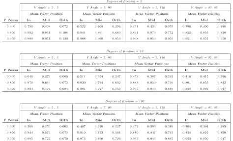
For the case k = 3, we have used ν = 2,10, and 100 and δ values that correspond

to partial F test powers of 0.4, .85, and .95. Figure 4 shows one case where C has the

restrictions −1 ≤ x1 ≤ 1, −.5 ≤ x2 ≤ .5, and 0.5 ≤ x3 ≤ 1. Note that the resulting cone

V can be controlled by the two angles between the two pairs of opposite faces of the cone.

In our simulation study we have used various combinations of the two angles from small 5◦_,

medium 90◦_{, to large 170}◦_{. The result of the simulations for this case is illustrated in the}

second panel of Table 2 for ν = 10.

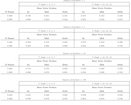
Finally, for the case k = 4 we have used ν = 1,5,10, and 100 and two δ values

corresponding to the partial F test powers of 0.4 and 0.9. We have varied the cone V based

on three angles, mainly by generalizing the method that we used for k = 2 and 3. It is

obviously not possible to draw the cone for this case. The results for this case are shown in

the third panel of Table 2 for ν= 10.

As mentioned earlier, the power of the new test depends on the direction of E(Z) =

W−1_β

2/σ relative to the position of the cone V, and in particular for our case the direction

of β2 (recall that we use W =I and σ = 1). To examine various positions of β2 relative to

V we have used the following directions for βT₂:

In Mid Orth

k = 2 (0,1) (1,1) (1,0)

k = 3 (0,0,1) (1,1,1) (1,1,0)

k = 4 (0,0,0,1) (1,1,1,1) (1,1,1,0)

Note that the vectors in the directions of (0,1), (0,0,1), and (0,0,0,1) are in the “centers”

of the conesV that we have used fork = 2,3 and 4, respectively (see e.g., Figures 3 and 4 for

of V (denoted by In), orthogonal to a vector in the center ofV (denoted by “Orth”), and in

between these to extremes (denoted by “Mid”).

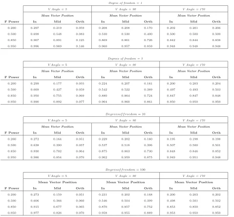
It is clear from the table that, for a given δ value, while the power of the partial F

test is fixed, the power of the new test increases when the angle between the mean vector

and the central direction of the cone decreases from 900 _{to 0}0_{. This phenomenon is more}

clear when the angles between the opposite faces of the cone V become small. So when the

angles between the opposite faces of the coneV are small and the mean vector is close to the

central direction of the cone, the new test usually has a large power that can be substantially

greater than the power of the partial F test. On the other hand, when the angles between

the opposite faces of the coneV are small and the mean vector is perpendicular to the central

direction of the cone, the new test usually has a small power that can be considerably smaller

than the power of the partial F test. But when the angles between the opposite faces of the

cone V are large (close to 1800_{) the variation in the power of the new test, when the angle}

between the mean vector and the central direction of the cone changes, is small, and the

powers of the new test are quite close to the power of the partial F test.

It is our view that the regionC should be determined by factors other than the power

property of the test. For example, in standard clinical studies the values of the important

covariates (such as age, blood pressure, etc.) are pre-defined by a set of inclusion/exclusion

criteria; patients are randomized into the study only if they satisfy the inclusion criteria.

Similarly, in survey studies, the range of the important covariates is also fixed in advance.

When considering risk factors for children, for instance, the covariate age is usually

con-strained to lie within two thresholds. Hence the natural choices of the intervals (al, bl) are

frequently known and fixed in advance of an experiment. Even if such thresholds are not

available prior to an experiment, natural boundaries may still be available and should be

Table 2: Power Comparison for the k = 2 case. The numerical values in the body of the table correspond to the power of the new test.

Degree of freedom = 1

V Angle = 5 V Angle = 90 V Angle = 170

Mean Vector Position Mean Vector Position Mean Vector Position

F Power In Mid Orth In Mid Orth In Mid Orth

0.200 0.297 0.219 0.059 0.208 0.208 0.170 0.202 0.201 0.206

0.500 0.698 0.548 0.083 0.530 0.530 0.400 0.500 0.500 0.500

0.850 0.967 0.891 0.125 0.869 0.861 0.726 0.842 0.844 0.838

0.950 0.996 0.969 0.146 0.960 0.957 0.859 0.948 0.948 0.948

Degrees of freedom = 5

V Angle= 5 V Angle = 90 V Angle = 170

Mean Vector Position Mean Vector Position Mean Vector Position

F Power In Mid Orth In Mid Orth In Mid Orth

0.200 0.299 0.177 0.055 0.224 0.207 0.161 0.200 0.203 0.204

0.500 0.669 0.427 0.059 0.542 0.522 0.389 0.497 0.493 0.503

0.850 0.950 0.755 0.069 0.880 0.864 0.724 0.847 0.847 0.848

0.950 0.990 0.892 0.077 0.964 0.960 0.861 0.950 0.950 0.950

Degreesof f reedom= 10

V Angle= 5 V Angle = 90 V Angle = 170

Mean Vector Position Mean Vector Position Mean Vector Position

F Power In Mid Orth In Mid Orth In Mid Orth

0.200 0.272 0.164 0.051 0.229 0.202 0.160 0.195 0.198 0.198

0.500 0.638 0.390 0.057 0.537 0.518 0.396 0.507 0.500 0.501

0.850 0.930 0.702 0.064 0.875 0.863 0.730 0.848 0.846 0.852

0.950 0.986 0.854 0.070 0.962 0.959 0.875 0.949 0.951 0.948

Degreeof f reedom= 100

V Angle= 5 V Angle = 90 V Angle = 170

Mean Vector Position Mean Vector Position Mean Vector Position F Power In Mid Orth In Mid Orth In Mid Orth

0.200 0.273 0.159 0.051 0.231 0.202 0.168 0.200 0.203 0.202

0.500 0.606 0.366 0.060 0.546 0.504 0.399 0.498 0.501 0.502

0.850 0.915 0.677 0.065 0.870 0.857 0.752 0.853 0.850 0.852

Table 3: Power Comparison for the k = 3 case. The numerical values in the body of the table correspond to the power of the new test.

Degrees of freedom = 2

V Angle = 5 , 5 V Angle = 5, 90 V Angle = 5, 170 V Angle = 85, 85

Mean Vector Position Mean Vector Position Mean Vector Position Mean Vector Position

F Power In Mid Orth In Mid Orth In Mid Orth In Mid Orth

0.400 0.730 0.408 0.072 0.522 0.408 0.296 0.451 0.424 0.350 0.398 0.400 0.388

0.850 0.992 0.861 0.106 0.941 0.861 0.683 0.891 0.879 0.772 0.852 0.855 0.838

0.950 0.999 0.951 0.130 0.988 0.960 0.950 0.968 0.950 0.950 0.951 0.951 0.950

Degrees of freedom = 10

V Angle = 5 , 5 V Angle = 5, 90 V Angle = 5, 170 V Angle = 85, 85

Mean Vector Position Mean Vector Positions Mean Vector Positions Mean Vector Position

F Power In Mid Orth In Mid Orth In Mid Orth In Mid Orth

0.400 0.640 0.279 0.060 0.511 0.354 0.247 0.452 0.387 0.322 0.416 0.412 0.396

0.850 0.970 0.660 0.073 0.920 0.794 0.602 0.883 0.850 0.746 0.861 0.855 0.842

0.950 0.994 0.794 0.084 0.981 0.917 0.753 0.965 0.949 0.886 0.954 0.956 0.947

Degrees of freedom = 100

V Angle = 5 , 5 V Angle = 5, 90 V Angle = 5, 170 V Angle = 85, 85

Mean Vector Position Mean Vector Position Mean Vector Position Mean Vector Position

F Power In Mid Orth In Mid Orth In Mid Orth In Mid Orth

0.400 0.569 0.250 0.062 0.487 0.330 0.227 0.452 0.380 0.316 0.404 0.394 0.385

0.850 0.944 0.575 0.073 0.910 0.753 0.564 0.880 0.837 0.745 0.854 0.855 0.850

Table 4: Power Comparison for the k = 4 case. The numerical values in the body of the table correspond to the power of the new test.

Degrees of freedom = 1

V Angle = 5, 5, 5 V Angle = 45, 45, 45

Mean Vector Position Mean Vector Position

F Power In Mid Orth In Mid Orth

0.400 0.720 0.461 0.101 0.471 0.453 0.340

0.900 0.999 0.943 0.244 0.953 0.940 0.816

Degrees of freedom = 5

V Angle = 5, 5, 5 V Angle = 45, 45, 45

Mean Vector Position Mean Vector Position

F Power In Mid Orth In Mid Orth

0.400 0.760 0.313 0.065 0.537 0.410 0.288

0.900 0.997 0.900 0.099 0.959 0.920 0.770

Degrees of freedom = 10

V Angle = 5, 5, 5 V Angle = 45, 45, 45

Mean Vector Position Mean Vector Position

F Power In Mid Orth In Mid Orth

0.400 0.710 0.274 0.062 0.546 0.400 0.278

0.900 0.992 0.679 0.091 0.959 0.908 0.763

Degrees of freedom = 100

V Angle = 5, 5, 5 V Angle = 45, 45, 45

Mean Vector Position Mean Vector Position

F Power In Mid Orth In Mid Orth

0.400 0.631 0.222 0.062 0.528 0.367 0.250

50< rest pulse <100, and so on.

For a chosen regionC, it is clear from this power study for what alternative hypothesis

β₂ 6=0 the new test tends to be more (less) powerful than the partial F test. Neither test is always more powerful than the other. But of course this observation/power study ignores

the fact the partialF test requires implicitly that model (1.1) holds over the entire range of

the covariates x2 which is difficult to justify for any real problem, while the new test only

requires that model (1.1) holds over the chosen region C of the covariates x2.

7

Conclusions

It is pointed out in this paper that the usual partialF test has in fact a naturally associated

confidence band, which is much more informative than the test itself. But this confidence

band is over the entire range of all the covariates. As regression models are true often only

over a restricted range of the covariates, the part of this confidence band outside this range

is useless and to guarantee an overall 1−α confidence level is wasteful of resources. A

narrower and hence more efficient confidence band is constructed over a restricted range of

the covariates.

The side product of this confidence band is a new test of the hypotheses (1.3). This

test is an improvement over the partial F test in the sense that the partial F test requires

implicitly that model (1.1) holds over the entire range of the covariatesx2 while the new test

only requires that model (1.1) holds over x2 ∈ C. Ignoring this weakness of the partial F

test, the power comparison between these two tests indicates for what alternative hypothesis

β6= 0 the new test can be either dramatically more or less powerful than the partial F test. It is our view that the prime factors in choosing the region C should be that model (1.1)

rather than the power property of the new test. The confidence bands are more informative

than the tests to allow us to make informed decision in model selection.

In this paper the covariates are assumed to be continuous variables and there is no

functional relationship among them. If some covariates are discrete variables or there are

functional relationships among the covariates the confidence band approach advocated here

can be adapted in a natural way via the region C in (4.1) and the corresponding V in (4.2).

The partial F test approach simply throws away this kind of information completely.

Finally, the covariate region C considered in this paper is restricted to a

hyper-rectangle, with the limits ai and bi being any real values. There may be situations that an

ellipsoidal covariate region is of interest. But it is not clear how to construct a simultaneous

confidence band over a given ellipsoidal covariate region in general. Casella and Strawderman

(1980) considered the construction of a simultaneous confidence band for a whole linear

regression model over an ellipsoidal covariate region that only has a particular center and a

particular shape. Further research in this direction is required.

Acknowledgements: We would like to thank two anonymous referees for many helpful comments.

REFERENCES

Casella, G. and Strawderman, W.E. (1980). Confidence bands for linear-regre

-ssion with restricted predictor variables. J. Amer. Stat. Assoc. 75, 862-868.

Fletcher, R. (1987). Practical methods of Optimization, Wiley: New York.

Kleinbaum, D.G., Kupper, L.L., Muller, K.E. and Nizam, A. (1998). Applied Regression

Liu, W., Jamshidian, M., and Zhang, Y. (2004). Multiple comparison of several linear

regression models. J. of the American Statistical Association, 99, 395-403.

Liu, W., Jamshidian, M., Zhang, Y. and Donnelly, J. (2005). Simulation-based simultaneous

confidence bands for a multiple linear regression model when the covariates are constrained.

J. of Computational and Graphical Statistics, to appear.

Miller, R.G. (1981), Simultaneous Statistical Inference, Springer-Verlag.

SAS Institute Inc. (1990). SAS/STAT User’s Guide, Version 6, Fourth edition, Volume 2

SAS InstituteInc., Cary, NC.