DOI 10.1007/s11045-006-0014-8
Decoupling and iterative approaches to the control
of discrete linear repetitive processes
B. Sulikowski · K. Gałkowski · E. Rogers · D. H. Owens
Received: 31 March 2006 / Revised: 26 September 2006 / Accepted: 5 December 2006 / Published online: 6 March 2007 © Springer Science+Business Media, LLC 2007
Abstract This paper reports new results on the analysis and control of discrete linear repetitive processes which are a distinct class of 2D discrete linear systems of both systems theoretic and applications interest. In particular, we first propose an exten-sion to the basic state-space model to include a coupling term previously neglected but which arises in some applications and then proceed to show how computationally efficient control laws can be designed for this new model.
Keywords Repetitive dynamics·Stability ·1D equivalent model· Dynamics decoupling·Iterative stabilization·LMIs
1 Introduction
The essential unique characteristic of a repetitive, or multipass, process is a series of sweeps, termed passes, through a set of dynamics defined over a fixed finite duration
B. Sulikowski (
B
)·K. GałkowskiInstitute of Control and Computation Engineering,
University of Zielona Góra, ul. Podgórna 50, 65-246 Zielona Góra, Poland e-mail: [email protected]
K. Gałkowski
e-mail: [email protected] E. Rogers
School of Electronics and Computer Science,
University of Southampton, Southampton SO17 1BJ, UK e-mail: [email protected]
D. H. Owens
known as the pass length. On each pass an output, termed the pass profile, is produced which acts as a forcing function on, and hence contributes to, the dynamics of the next pass profile. This, in turn, leads to the unique control problem in that the output sequence of pass profiles generated can contain oscillations that increase in ampli-tude in the pass-to-pass direction.
To introduce a formal definition, letα < +∞denote the pass length (assumed constant). Then in a repetitive process the pass profile yk(p), 0≤p≤α−1, generated
on pass k acts as a forcing function on, and hence contributes to, the dynamics of the next pass profile yk+1(p), 0≤p≤α−1, k≥0.
Physical examples of repetitive processes include long-wall coal cutting and metal rolling operations (Edwards, 1974). Also in recent years applications have arisen where adopting a repetitive process setting for analysis has distinct advantages over alternatives. Examples of these so-called algorithmic applications include classes of iterative learning control (ILC) schemes (Owens, Amann, Rogers, & French,2000) and iterative algorithms for solving nonlinear dynamic optimal control problems based on the maximum principle (Roberts,2002). In the case of ILC for the linear dynam-ics case, the stability theory for so-called differential and discrete linear repetitive processes can be used to undertake a rigorous stability/convergence theory for a pow-erful class of such algorithms. In particular, it makes explicit the link between error convergence and along the trial dynamics in a manner which is not possible using, for example, other 2D systems model structures, e.g.Kurek, & Zaremba(1993).
Attempts to control these processes using standard (or 1D) systems theory/algorithms fail (except in a few very restrictive special cases) precisely be-cause such an approach ignores the two features that define their inherent 2D systems structure. These are information propagation from pass-to-pass (k direction) and along a given pass (p direction) and resetting of the initial conditions before the start of each new pass. In which context, it is known (Owens, & Rogers,1999) that the structure of these alone can cause instability.
In seeking a rigorous foundation on which to develop a control theory for these processes, it is natural to attempt to exploit structural links which exist between, in particular, the class of so-called discrete linear repetitive processes and 2D linear sys-tems described by the extensively studied Roesser (1975) or Fornasini and Marchesini (1978) state-space models. In fact, however, there are dynamics arising in repetitive processes which have no Roesser or Fornasini–Marchesini model interpretations. For example, it can happen that the previous pass profile is modified over its complete duration before the production of the next pass profile begins, e.g. in long-wall coal cutting where this so-called inter-pass smoothing is caused by the machines weight as it it brought to rest on the new cut floor profile before the start of the new pass of the coal face. Such dynamics cannot be included in a Roesser or Fornasini Marchesini model setting and the novel results in this paper include how a discrete model of such action can be accommodated in repetitive process analysis and control law design.
In common with a large range of other areas in systems theory, recent years has seen the emergence of Linear Matrix Inequality (LMI) based techniques in the anal-ysis of very important sub-classes of linear repetitive processes (see, e.g.,Galkowski, Rogers, Xu, Lam, & Owens,2002;Galkowski, Paszke, Sulikowski, Rogers, & Owens,
led, unlike other currently available alternatives, to the development of stability tests which also provide a basis for the design of physically meaningful control laws for both stability and performance. Here we show how such tools can be used to great effect in the control of the previously not considered repetitive process dynamics considered in this paper.
Throughout this paper M>0(<0)denotes a real symmetric positive (negative) definite matrix.
2 Background
The state-space model of a so-called extended discrete linear repetitive process is described by the following state-space model over 0≤p≤α−1, k≥0,
xk+1(p+1)=Axk+1(p)+Buk+1(p)+
α−1
j=0
Bjyk(j),
yk+1(p)=Cxk+1(p)+Duk+1(p)+
α−1
j=0
Djyk(j). (1)
Here on pass k, xk(p)is the n×1 state vector, yk(p)is the m×1 pass profile vector,
and uk(p)is the r×1 vector of control inputs.
To complete the process description, it is necessary to specify the boundary con-ditions, i.e. the state initial vector on each pass and the initial pass profile. Here no loss of generality arises from assuming xk+1(0)=dk+1, k≥0, where dk+1is an m×1
vector with known constant entries, and y0(p)=f(p), where f(p)is an m×1 vector
whose entries are known functions of p over 0≤p≤α−1. For ease of presentation, we will make no further reference to the boundary conditions in this paper.
Motivation for considering processes of the form (1) arises from applications where the current pass profile at any point along the pass is a function of more than one point on the previous pass. For example, in mining systems, the repetitive process dynamics arise from the fact that, as the current pass profile is being produced, the machine involved rests on the previous pass profile and once the end is reached it is returned to the starting position and then ‘pushed over’ to rest on the newly produced pass profile ready for the start of the next pass. Hence, it is clear that the complete previous pass profile in this case will make a significant contribution to the construc-tion of the current pass profile at any point p on the current pass. Consequently the resulting effects on the dynamics must be accounted for in any ‘realistic’ mathematical model.
Suppose that for p=0, 1,. . .,α−1
Bj=
B0, j=p,
0, j=p (2)
and also
Dj=
D0, j=p,
0, j=p. (3)
Then in this case, the model of (1) reduces to that first introduced inRogers, & Owens
(1992), i.e.
xk+1(p+1)=Axk+1(p)+Buk+1(p)+B0yk(p),
yk+1(p)=Cxk+1(p)+Duk+1(p)+D0yk(p). (4)
In this paper we will refer to this last model as a standard and the model of (1) as an extended discrete linear repetitive process respectively.
Consider the following partial ordering of two tuple integers
(i, j)≤(k, p), if i≤k and j≤p, (i, j)=(k, p), if i=k, j=p,
(i, j) < (k, p), if(i, j)≤(k, p)and(i, j)=(k, p).
Then the dynamics of the discrete linear repetitive processes considered in this paper can be visualized as evolving over the rectangle
De:= {(k, p): k≥0, 0≤p≤α−1}.
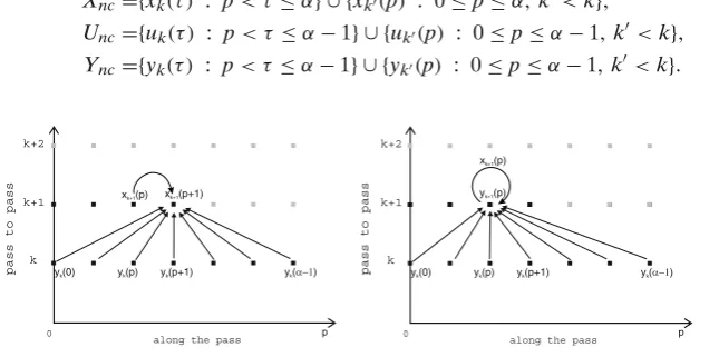
Figure1shows the updating structure of the state and pass profile vectors in (1) (which clearly includes that of (4) as a special case).
Suppose also that it is required to ensure stability for a given example. Then in terms of control law actuation, information in the following sets has already been generated at point p on pass k and hence available for use in a control law
Xnc={xk(τ) : p< τ≤α} ∪ {xk(p) : 0≤p≤α, k<k},
Unc={uk(τ) : p< τ ≤α−1} ∪ {uk(p) : 0≤p≤α−1, k<k}, Ync={yk(τ) : p< τ≤α−1} ∪ {yk(p) : 0≤p≤α−1, k<k}.
(5)
along the pass p 0
k
k+1 x (p)k+1 x (p+1)k+1
y (0)k y (p)k y (p+1)k y (k )
k+2
yk+1(p)
xk+1(p)
pass to pas
s
pass to pass
along the pass p 0
k k+1
y (0)k y (p)k y (p+1)k y (k )
k+2
[image:4.439.46.369.444.604.2]For processes described by (4) it is (as noted previously in this paper) possible to solve some control related problems by exploiting their inherent 2D linear sys-tems structure and, in effect, adapt tools/results first developed for 2D linear syssys-tems described by the extensively studied Roesser (1975) and Fornasini and Marchesini (1978) state-space models. In cases where this approach is not applicable, such as pass profile controllability (Galkowski, Rogers, & Owens,1998) which has no Roes-ser or Fornasini–Marchesini model equivalent, the 1D equivalent model (Galkowski, Rogers, & Owens,1998) has provided the analysis basis on which to characterize this property in terms of matrix rank tests and easily implemented stability tests respectively. Here we investigate the role of such an equivalent model for processes described by (1), where its construction is a straightforward extension of that for processes described by (4), and hence only the main steps are detailed here.
Set l= k+1 and vl+1(p) =yl(p)in (1) and introduce the so-called global state,
input and pass profile vectors (termed super-vectors here) of dimensions nα×1, rα×1 and mα×1, respectively, as
X(l):=
⎡ ⎢ ⎢ ⎢ ⎢ ⎢ ⎣
xl(1) xl(2) xl(3)
.. .
xl(α)
⎤ ⎥ ⎥ ⎥ ⎥ ⎥ ⎦
, U(l):=
⎡ ⎢ ⎢ ⎢ ⎢ ⎢ ⎣
ul(0) ul(1) ul(2)
.. .
ul(α−1)
⎤ ⎥ ⎥ ⎥ ⎥ ⎥ ⎦
, V(l):=
⎡ ⎢ ⎢ ⎢ ⎢ ⎢ ⎣
vl(0) vl(1) vl(2)
.. .
vl(α−1)
⎤ ⎥ ⎥ ⎥ ⎥ ⎥ ⎦ .
Then the 1D equivalent model is
X(l)=αV(l)+αU(l)+0αdl,
V(l+1)=αV(l)+αU(l)+0αdl, (6)
where
0α:=
⎡ ⎢ ⎢ ⎢ ⎢ ⎢ ⎣ A A2 A3 .. . Aα ⎤ ⎥ ⎥ ⎥ ⎥ ⎥ ⎦
, 0α:=
⎡ ⎢ ⎢ ⎢ ⎢ ⎢ ⎣ C CA CA2 .. .
CAα−1
⎤ ⎥ ⎥ ⎥ ⎥ ⎥ ⎦ ,
α:= ⎡ ⎢ ⎢ ⎢ ⎢ ⎢ ⎣
B 0 0 . . . 0
AB B 0 . . . 0
A2B AB B . . . 0
..
. ... ... . .. ...
Aα−1B Aα−2B Aα−3B. . .B
⎤ ⎥ ⎥ ⎥ ⎥ ⎥ ⎦ ,
α:= ⎡ ⎢ ⎢ ⎢ ⎢ ⎢ ⎢ ⎢ ⎢ ⎣
B0 B1 B2 . . . Bα−1
B0+AB0 B1+AB1 B2+AB2 . . .Bα−1+ABα−1 2
i=0AiB0 i2=0AiB1 2i=0AiB2 . . . 2i=0AiBα−1 3
i=0AiB0 i3=0AiB1 3i=0AiB2 . . . 3i=0AiBα−1
..
. ... ... . .. ...
α−1
i=0 AiB0 iα=−01AiB1 iα=−01AiB2. . . iα=−01AiBα−1
α:= ⎡ ⎢ ⎢ ⎢ ⎢ ⎢ ⎢ ⎢ ⎢ ⎢ ⎣
D0 D1 D2 . . . Dα−1
CB0+D0 CB1+D1 CB2+D2 . . . CBα−1+Dα−1
1
i=0CAiB0+D0 1i=0CAiB1+D1 1i=0CAiB2+D2 . . . 1i=0CAiBα−1+Dα−1 2
i=0CAiB0+D0 2i=0CAiB1+D1 2i=0CAiB2+D2 . . . 2i=0CAiBα−1+Dα−1
. . . . . . . . . . .. ...
α−2
i=0 CAiB0+D0 iα=−02CAiB1+D1 iα=−02CAiB2+D2. . . iα=−02CAiBα−1+Dα−1
⎤ ⎥ ⎥ ⎥ ⎥ ⎥ ⎥ ⎥ ⎥ ⎥ ⎦ , α:= ⎡ ⎢ ⎢ ⎢ ⎢ ⎢ ⎣
D 0 0 . . . 0
CB D 0 . . . 0
CAB CB D . . . 0
..
. ... ... . .. ...
CAα−2B CAα−3B CAα−4B. . .D
⎤ ⎥ ⎥ ⎥ ⎥ ⎥ ⎦ . (7)
Next, we introduce the required parts of the stability theory for constant pass length linear repetitive processes and develop some new results on dynamic decoupling (defined in context in the next section).
3 Stability and stabilization: the standard model case
The stability theory (Rogers, & Owens,1992) for linear repetitive processes is based on an abstract model of the process dynamics in a Banach space setting and consists of two distinct concepts, termed asymptotic stability and stability along the pass, respec-tively. Recalling the unique control problem for these processes, asymptotic stability demands that bounded (defined in terms of the norm on the underlying signal space) input sequences (formed from control inputs and disturbances which enter on the current pass) produce bounded sequences of pass profiles over the, finite and fixed by definition, pass length. Also if this property holds then the sequence of pass profiles produced is guaranteed to converge in the pass-to-pass direction to a so-called steady or limit profile which in the case of the processes considered here are described by a 1D discrete linear systems state-space model.
For the remainder of this section, we consider only processes described by (4) since the extension to processes described by (1) is immediate (we will exploit dynamic decoupling as defined below in the next section). First note that asymptotic stability holds if, and only if, r(D0) <1, where r(·)denotes the spectral radius of its argument.
Also, with D =0 for simplicity, the 1D model describing the resulting limit profile dynamics has state matrix AlP := A+B0(Im−D0)−1C. Hence it is possible for a
process to be asymptotically stable yet the resulting limit profile is ‘unstable along the pass’ in the 1D systems sense, i.e. r(AlP) ≥ 1. A simple example here is when A = −0.5, B = 1, B0 = −0.5+β, C = 1, D= D0 = 0, where the real scalarβ is
chosen such that|β| ≥1.
requirement that r(A) <1, since this matrix describes the evolution of the dynamics along a pass. This is indeed true but, as the above example demonstrates, it still does not guarantee that unstable limit profile dynamics cannot occur. The extra condi-tion required here is most appropriately expressed as the requirement that, assuming {A, B0}is controllable and{C, A}observable, all eigenvalues of the transfer function matrix
G0(z):=C(zIn−A)−1B0+D0 (8)
have modulus strictly less than unity for all|z| =1.
It is also possible to give a physically based interpretation of these properties and the difference between them. Consider first asymptotic stability in the presence of no control input terms. Then at p=0 we have yk(0)=Dk0y0(0), k≥1. Hence asymptotic
stability can be interpreted as requiring that the sequence of pass initial profile vectors must not become unbounded with k. For stability along the pass consider for simplic-ity the single-input single-output case with zero state initial vector sequence and zero control input. Then the process dynamics can be written as yk(z)= G0k(z)y0(z)and
hence we see that this property requires that each frequency component of the initial pass profile is attenuated from pass-to-pass at a geometric rate.
Suppose also that it is required to ensure stability for a given example. Then in terms of control law actuation, all the information in the sets of (5) is available for use. In implementation terms, however, there is clearly benefit to be achieved from using a control law which requires the minimal amount of information from these sets. Moreover, earlier work (Rogers, & Owens,1992) has shown that, except in a few very restrictive special cases, the control law used must be actuated by a combination of current pass information and ‘feedforward’ information from the previous pass to guarantee even stability along the pass with the control law applied. Note also here that in the ILC application area the previous pass output vector (or a trial in ILC terminology) is an obvious signal to use as feedforward action.
One control law with this structure is of the following form over 0≤p≤α−1, k≥0
uk+1(p)=Hxxk+1(p)+Hyyk(p):=H
xk+1(p) yk(p)
, (9)
where Hxand Hyare appropriately dimensioned matrices to be designed. Note that
(9) can be partitioned into two following control laws (depending on which part of model is to be influenced), i.e.
uk+1(p)=Hyyk(p)+ ˆuk+1(p) (10)
or
uk+1(p)=Hxxk+1(p)+ ˆuk+1(p), (11)
where nowuˆk+1(p)denotes an auxiliary control input which is available for the further
use (if required).
The stability properties of processes described by (4) can be compactly summarized in terms of the so-called augmented plant matrix
ϒ:=
A B0
C D0
and under the action of a control law of the form (10) this is mapped to
ϒc:=
A B0+BHy
C D0+DHy
and under (11) to
ϒc:=
A+BHx B0 C+DHx D0
(For the extended model (1) only the first of these mappings holds).
It now follows immediately that under the action of (10), the matrix D0
govern-ing asymptotic stability is mapped to D0+DHy and hence the controlled process
has this property if, and only if, the pair{D0, D}is controllable in normal 1D sense.
Similarly, using (11), the matrix A is mapped to A+BHxand it follows immediately
that this control law can achieve the necessary condition for stability along the pass that r(A+BHx) <1 if, and only if, the pair{A, B}is controllable in the normal 1D sense. Note also that the application of (10) or (11) always maps the matrix B0or C,
respectively, and hence the possibility of using it simplify the dynamics of the resulting controlled process by decoupling the pass state and pass profile updating equations in the manner detailed next.
Consider first (10) and suppose that it is possible to achieve
B0 :=B0+BHy=0 (12)
by the suitable choice of Hy. Then the state dynamics on the current pass are
com-pletely decoupled from the previous pass profile and a simplified updating structure holds. In particular, given the pass state initial vector sequence{dk}k≥1and the control
input sequence to be applied, the state dynamics on each pass can be computed and then the corresponding pass profile sequence, i.e. in Figure1simplified to this case horizontal (state) and vertical (pass profile) updating become independent of each other. Also asymptotic stability holds provided we can also choose Hysuch that
r(D0) <1, D0 :=D0+DHy. (13)
Suppose now that (11) is applied and it is also possible to achieve
C :=C+DHx=0. (14)
Then the state dynamics on the current pass are completely decoupled from the pre-vious pass profile and a simplified updating structure then holds. In particular given the pass initial profile y0(p)and the control input sequence the pass profile sequence
can be computed directly (and then the pass state vector sequence if required). Also it is possible that (11) can be designed such that
r(A) <1, A :=A+BHx. (15)
Theorem 1 Suppose that a control law of the form (11) is applied to a discrete linear repetitive process described by (4). Then (14) and (15) simultaneously hold if, and only if, there exist matrices Px>0, Gx, and Nxsuch that the following LMI holds
−Px AGx+BNx GTxAT+NxTBT Px−Gx−GTx
<0, (16)
CGx+DNx=0. (17)
When this condition holds, Hxcan be computed as
Hx =NxG−x1.
Theorem 2 Suppose that a control law of the form (10) is applied to a discrete linear repetitive process described by (4). Then (12) and (13) simultaneously hold if, and only if, there exist matrices Py>0, Gyand Nysuch that the following LMI holds
−Py D0Gy+DNy GTyDT0 +NyTDT Py−Gy−GTy
<0, (18)
B0Gy+BNy=0. (19)
When this condition holds, Hycan be computed as
Hy =NyG−y1.
The following result concerning stability along the pass can also be stated. Theorem 3 Suppose that a control law of the form (9) is applied to a discrete linear repetitive process described by (4). Then the resulting controlled process is stable along the pass if
(a) (16) holds,
(b) (18) holds,
(c) C=0 orB0=0.
Proof The inequalities (16) and (18) are equivalent to r(A) <1 and r(D0) <1,
respec-tively (Sulikowski, Galkowski, Rogers, & Owens,2005). Now consider the controlled process version of (8), i.e.
G0(z):=C(zIn−A)−1B0+D0.
Then clearlyC=0 orB0=0 guarantees
r(G0(z))=r(D0 ) <1.
The analysis above is, of course, subject to several strong limitations which may hinder its applicability. First, the two matrix equations in this last result must be solved and the existence of a solution requires that
rank(D)=rank([D, CGx])
and
The point here is that the decision matrices Gxand Gyin the LMIs are also the part of
the conditions for the existence of solutions which can cause problems. If no solutions of (17) and (19) exist, then one possibility is to attempt approximate decoupling by minimizing a norm applied to CGx+DNxand B0Gy+BNy.
This decoupling based approach can also be applied to the model of (1) but stability along the pass is a much more involved question. Moreover, design for asymptotic stability could include the need to work with (potentially) very large dimensioned matrices. We show in the next section, however, that this problem can be avoided by adopting a different design strategy. Finally, note that uncertainty in the model matri-ces in the above design can also be treated using known techniques. In particular, if there is uncertainty in C and D for the first case and B0 and B for the second then
analysis based on uncertainty models with a known norm bounded structure (see, for example, Galkowski et al.,2003) or polytopic form (Cichy, Galkowski, Kummert, & Rogers,2005) extends directly—the equality constraints (17) and (19), respectively, do not change their forms and (16) and (18) respectively need only be rewritten in the form of the considered uncertainty structure.
4 Stability and stabilization analysis: the extended model case
Consider first asymptotic stability of the extended model where the situation is clearly much more complicated than for the standard model. There is, however, a route for-ward based on the fact that asymptotic stability in this case is equivalent to requiring
r(α) <1 in the 1D equivalent model (which can be proved as inRogers, Galkowski, Gramacki, Gramacki, & Owens,2002for the case of dynamic boundary conditions.)
This is a very powerful result and the only real difficulty with it is the (potentially) very large dimensions of the matrix involved. Note also that major numerical errors can occur during the construction of the 1D equivalent model due to the need to form powers of the matrix A, especially when r(A) >1.
Numerical difficulties could also arise in terms of control law design to ensure asymptotic stability. To explain this point, note that for processes described by (4), asymptotic stability can be achieved (here we assume that this is possible) under a control law of the form (9) (with Hx = 0 for simplicity) by choosing the matrix Hy
such that r(D0+DHy) <1. In the case of processes described by (1), however, this is not possible and here we show that an alternative is to employ the 1D equivalent model and seek to design a control law of the form
U(l)=KV(l) (20)
such that r(α+αK) <1. This control law is actuated by all points along the previ-ous pass where as (9) is only single point actuated. Given that in the model of (1) it is all points along the previous pass which contribute to the dynamics at a single point on the current pass (plus the fact that asymptotic stability deals with information in the pass-to-pass (k) direction) it is to be expected that a control law with single point actuation will be relatively weak in this case.
As the first step in developing an efficient design algorithm for (20) to ensure asymptotic stability, we proceed via an LMI interpretation arising from the fact that
−P T
αP
Pα −P
<0. (21)
Hence we have the following necessary and sufficient condition for asymptotic stabil-ity under the action of the control law (20).
Theorem 4 Suppose that the 1D equivalent model (6) is used to design a control law of the form (20) for a discrete linear repetitive process described by (1). The controlled process is asymptotically stable if, and only if,∃matrices Q> 0 and L such that the
following LMI holds
−Q QTα +LTTα
αQ+αL −Q
<0. (22)
Also if this condition holds then K in (20) can be computed as
K=LQ−1. (23)
Proof The controlled process is asymptotically stable (using the Lyapunov stability
inequality for 1D discrete linear systems with state matrixα, input matrixα and state feedback matrix K) if, and only if,
(α+αK)TP(α+αK)−P<0, (24) where P> 0. Applying the Schur’s complement formula for matrices and pre- and post-multiplying the result as detailed next
I 0
0 P
−P (α+αK)T α+αK −P−1
I 0
0 P
<0 (25)
yields
−P (α+αK)TP
P(α+αK) −P
<0. (26)
Next, set Q=P−1and pre- and post-multiply (26) by the diagonal matrix diag{Q, Q}
to obtain
−Q Q(α+αK)T
(α+αK)Q −Q
<0. (27)
Use of (23) now yields the LMI of (22) and the proof is complete.
A difficulty in applying this result may arise since Q is a LMI decision matrix and simultaneously is used to compute the control law matrix K. The next result is better in this respect and is based on the 1D case as inPeaucelle, Arzelier, Bachelier, & Bernussou(2000).
Theorem 5 Suppose that the 1D equivalent model (6) is used to design a control law of the form (20) for a discrete linear repetitive process described by (1). Then the con-trolled process is asymptotically stable if, and only if,∃matrices P>0 and G, L such
that the following LMI holds
−P αG+αL GTTα+LTTα P−G−GT
Also if this condition holds, a stabilizing K is given by
K=LG−1. (29)
Proof For necessity assume that G=Q and then (28) reduces to (22). For sufficiency, left multiply (28) by[I|α+αLG−1](note that G is invertible since G+GT >0) and right multiply the result by the transpose of this matrix to obtain (24).
Both of the design methods given above require the solution of possibly very large dimensioned LMIs which is well known to be difficult to do using modern solvers. Next, we show that this problem can be overcome in some cases of direct interest here by exploiting the decoupling results of the previous section. In particular, suppose that the current pass state vector is decoupled from the pass profile updating equation in (1) using the control law uk+1(p)=Hxxk+1(p)+ ˆuk+1(p), such that C+DHx =0
(whereuˆk+1(p)is an auxiliary current pass control input vector). (Note that in the
design algorithm which follows C and D must be exactly known and the extension to robustness analysis as discussed at the end of the previous section can only be applied here when the uncertainty is not present in these matrices.)
The resulting controlled process state-space model after the control law has been designed is
xk+1(p+1)=(A+BHx)xk+1(p)+Buˆk+1(p)+
α−1
j=0
Bjyk(j),
yk+1(p)=Duˆk+1(p)+
α−1
j=0
Djyk(j) (30)
and in the 1D equivalent model we have that
α=
⎡ ⎢ ⎢ ⎢ ⎣
D0 D1 D2 . . . Dα−1 D0 D1 D2 . . . Dα−1
..
. ... ... . .. ...
D0 D1 D2 . . . Dα−1
⎤ ⎥ ⎥ ⎥ ⎦, α=
⎡ ⎢ ⎢ ⎢ ⎣
D 0 0 . . . 0
0 D 0 . . . 0
..
. ... ... . .. ...
0 0 0 . . . D
⎤ ⎥ ⎥ ⎥ ⎦. (31)
Now we have the following easily proved result which, in effect, is a computationally more efficient test for asymptotic stability.
Lemma 1 The matrixα of (31) has(α−1)m zero eigenvalues and the remaining m are those of the matrix αj=−01Dj.
The form ofαhere can also be exploited in the design of a control law of the form ˆ
U(l)=KV(l), (32)
whereUˆ(l) is the 1D equivalent model super-vector corresponding touˆk+1(p), to
K=
⎡ ⎢ ⎢ ⎢ ⎣
K0 K1 K2 . . . Kα−1 K0 K1 K2 . . . Kα−1
..
. ... ... ... ...
K0 K1 K2 . . . Kα−1
⎤ ⎥ ⎥ ⎥
⎦, (33)
which yields a 1D equivalent model with state matrix ˜
α =α+αK. (34)
Then we have the following result.
Theorem 6 Suppose that a control law of the form uk+1(p)=Hxxk+1(p)+ ˆuk+1(p)is applied to a discrete linear repetitive process described by (1) and has been designed such that (30) holds. Suppose also that (30) is replaced by its 1D equivalent model (6) which is then used to design a control law of the form (32) (i.e.Uˆ(l)=KV(l)) applied with a K of the form (33). Then the resulting controlled process is asymptotically stable if, and only if,∃matrices P>0, G, Lj, j=0, 1,. . .,α−1 such that the following LMI holds
⎡ ⎢ ⎢ ⎢ ⎢ ⎢ ⎣
−P
α−1
j=0
DjG+DLj
α−1
j=0
GTDTj +LTj DT
P−G−GT
⎤ ⎥ ⎥ ⎥ ⎥ ⎥ ⎦<
0. (35)
Also if this condition holds, block entry Kjin the control law matrix K of (33) is given by
Kj=LjG−1, ∀j=0, 1,. . .,α−1. (36)
Proof First, setD= αj=−01Dj,K= jα=−01KjandL= αj=−01Lj. Then the resulting
controlled process is asymptotically stable if, and only if,
(D+DK)TW(D+DK)−W <0, (37)
where W>0. Next make an obvious application of the Schur’s complement formula and pre- and post-multiply the result by
I 0
0 W
to obtain
−W (D+DK)TW
W(D+DK) −W
<0. (38)
Now set P=W−1and pre- and post-multiply (38) by the diagonal matrix diag{P, P}
to obtain
−P P(D+DK)T (D+DK)P −P
<0 (39)
or, withK=LP−1,
−P PDT+LTDT
DP+DL −P
Now we have to establish that (40) is equivalent to (35), where this last condition can be replaced by
−P DG+DL GTDT+LTDT P−G−GT
<0. (41)
To show necessity, assume G = P and note that (41) becomes (40) since the LMI is symmetric. For sufficiency, left multiply (41) by[I|D+DLG−1](note that G is invertible since G+GT >0) and right multiply the result by its transpose to obtain (37). Next note that
K=LG−1=
⎛ ⎝α−1
j=0 Lj
⎞ ⎠G−1 =
α−1
j=0
(LjG−1)=
α−1
j=0
Kj (42)
and (35) ensures that the control law matrixKis such that
r
⎛ ⎝ ⎛ ⎝α−1
j=1 Dj
⎞ ⎠+DK
⎞
⎠<1, (43)
which, on applying the result of Lemma 1, is equivalent to r(˜α) <1. This completes the proof.
Remark 1 Note here that the LMI to be solved in this last result is, in general, of much less dimension than that of Theorem 5. In particular, we have to compute an
mα×mαdecision matrix in the LMI of Theorem 5 and in that of Theorem 6 an m×m
matrix, where most oftenα(the pass length) is much greater than m (the number of entries in the pass profile vector).
A simplified form of the above result arises when it is assumed that
Kij= ˆK, i, j=0, 1,. . .,α−1. (44) Also if this condition holds then it is easy to conclude thatK=αK, and from (42ˆ )L of (35) satisfiesL=αL. Hence we can then useˆ
K=
⎡ ⎢ ⎢ ⎢ ⎢ ⎣ ˆ
K Kˆ Kˆ . . . Kˆ
ˆ
K Kˆ Kˆ . . . Kˆ
..
. ... ... ... ... ˆ
K Kˆ Kˆ . . . Kˆ
⎤ ⎥ ⎥ ⎥ ⎥
⎦. (45)
In summary, therefore, we have developed a procedure for control law design to achieve asymptotic stability of processes described by (1). The first step is to use preliminary control action to decouple the current pass state vector from the pass profile updating equation (which, however, is not always possible). This step does not reduce the dimension of, in particular, the matrixα but crucially greatly simplifies its spectrum. It is this fact which simplifies the final control law design.
∞ := limα→∞α. Then it can be argued directly from the abstract model based theory that stability along the pass holds if, and only if, r(∞) <1. This in turn, is equivalent to r( ∞j=0Dj) <1 which is more convenient for numerical evaluation.
5 Successive stabilization
The analysis of the previous section has produced a systematic method of ensuring asymptotic stability using the 1D equivalent model. A consequence of this, however, is that the inherent 2D linear systems structure of these processes has been subsumed into the 1D model and in some cases of interest it will be beneficial to retain this structure. Also to meet the decoupling specifications of the previous analysis, extra conditions are necessary which will not always hold. Conversely, direct use of Theo-rem 4 or 5 could lead in some cases to computations involving matrices of extTheo-remely high dimensions and hence the strong possibility of overflow and underflow errors in intermediate steps which can completely destroy the numerical reliability of the calculation process. (The problem here arises from the multiplication of the input, pass profile and state vector dimensions by the value of the pass length during the construction of the 1D equivalent model.)
As an alternative, we now develop the so-called successive stabilization approach. In effect, this first replaces the potentially huge dimensioned problem with one of less dimensions and then iteratively improves it to the full pass length subject to the requirement that the outcome of each stage must result in a state-space model which has the structure of a discrete linear repetitive process (this is not guaranteed in the cases where Theorem 4 or 5 can be applied).
To improve the iterative solution algorithm, the preliminary step of stabilizing the matrix A in the 1D discrete linear systems sense when r(A)≥1 can lead to a reduction in the number of iterations needed to obtain the required result. Note also that suc-cessive stabilization is not an alternative solution in cases when Theorem 4 or 5 does not hold. Rather the aim is to obtain an efficient and numerically reliable solution in the case when at least one of these results holds but is not computationally feasible with a high degree of accuracy.
To proceed, suppose that the control law matrix K applicable in (20) is assumed to be of the form (33), where this ensures that the controlled process retains the structure of (1). Hence K can be treated as a set of 2D controllers Ki, i =0,. . .,α−1, which
influence the dynamics from pass-to-pass.
The structure of (33) for K can be achieved by setting
G=
⎡ ⎢ ⎢ ⎢ ⎣
G0 0 . . . 0
0 G1 . . . 0
..
. ... ... ... 0 0 . . . Gα−1
⎤ ⎥ ⎥ ⎥
⎦ (46)
and
L=
⎡ ⎢ ⎢ ⎢ ⎣
L0 L1 L2 . . . Lα−1 L0 L1 L2 . . . Lα−1
..
. ... ... ... ...
L0 L1 L2 . . . Lα−1
⎤ ⎥ ⎥ ⎥
in the condition of Theorem 5. Then K0 = L0G−01, K1 = L1G−11,. . ., Kα−1 = Lα−1G−α−11, and alsoαcan be written in the formα = [ij], where
ij=
⎧ ⎪ ⎨ ⎪ ⎩
Dj+DKj, i=1, j=0, 1,. . .,α−1,
Dj+DKj+ i−1
t=0
(CAtBj+CAtBKj), i=2, 3,. . .,α, j=0, 1,. . .,α−1
= ⎧ ⎪ ⎪ ⎨ ⎪ ⎪ ⎩
Dj, i=1,
Dj+ i−1
t=0
(CAtBj), i=2, 3,. . .,α−1.
(48)
Hence, it follows immediately that the controlled process with the matrix K given by (33) has a state-space model of the form (1) withA= A,B= B, C = C, D= D
and
Bi=Bi+BKi, Di =Di+DKi, i=0, 1,. . .,α−1. (49) The basic idea of so-called successive stabilization is that we first make the process asymptotically stable over a short pass length and then subsequently augment this design by increasing the pass length by using only control action which preserves the original repetitive process state-space model structure. This approach to design also avoids the need to work with matrices with very large dimensions.
The design procedure is as follows.
Step 1 Choose an initial pass lengthα1 < α, and h the number of points added in
each iteration such that there exists a natural number q satisfyingα−α1=qh.
Set an iteration counter v=1.
Step 2 Construct α1 using (7) withα = α1 and check if r(α1) < 1. If yes, go to
Step 5.
Step 3 Use (28) and (29) to compute the appropriate control law matrices K0, K1,. . ., Kα1−1for the partial pass of the lengthα1. Set Kα1, Kα1+1, . . ., Kα−1=0 and
calculate the full modified system matrix˜αof (34).
Step 4 Check if r(˜α) <1, and if this is true terminate the procedure. If not, go to the next step.
Step 5 Check ifα1+h> αholds. If yes, terminate the procedure since asymptotic
stability for the controlled process cannot be achieved by this method. If no, increase v by 1, setα1 :=α1+h and return to Step 2.
Remark 2 Note that above algorithm is always at least as effective as stabilization based on direct use of the matrixα. To see this, setα1=αin the first step. Also if the
initial stabilization problem size isα1< α, and it is impossible to achieve stabilization
for such a chosen pass length, then executing Step 5 finally gives stabilization based onα.
Remark 3 For sufficiently largeα and small α1 and h the evaluation of the above
algorithm can take a very long time but overall we have found that it compares very favourably with solving the stabilization problem with the fullα.
6 Examples
Example 1 Consider the particular case of (1) whenα=20 and
A=
⎡
⎣ 1.990.0 −0.00.96 −0.01.87 −2.36 −2.82 −0.32 ⎤ ⎦,
B=
⎡
⎣2.240.0 1.540.0 −1.432.13 0.92−2.03 1.18
⎤ ⎦,
B :=B0 B1 . . .B19
= ⎡
⎣−0.01.44−−0.962.54−0.02.85−0.00.71 1.860.0 −1.33 1.47 0.0 0.881.87 0.0 0.0 2.81 2.20−0.87 0.0 2.07 0.0 0.10 2.62 0.0 2.40 3.0 0.53−0.29 0.56 −0.09−2.36−2.63 0.0−2.80 0.74 2.21 0.0 0.03 −1.88−0.33 0.0 0.0 0.0 1.92 1.77 0.0 2.58 0.14 1.33 0.0 1.0 0.0 0.0−1.27 2.83 0.67 1.04 0.51 0.03 0.0 0.0 1.03 −0.37−2.15 0.82 2.95−1.59−0.96
0.0 0.50 0.0 0.0 1.24 0.56 0.0 0.0 2.02 −2.84 0.0 −2.96 0.0−2.22 0.0 0.0 0.0 1.08−0.84−0.32 −2.02−0.47−1.45 2.09 0.0 0.68 0.25 0.07 2.60 0.0
1.94 0.76 0.60 0.0 −0.81 0.0 2.87−1.85−0.15−0.13 −2.19 0.0 −1.18−1.67−0.98−2.63 0.0 0.0 0.99 0.0
⎤ ⎦,
C=
1.38 1.69 −2.21 0.0 0.0 1.62
,
D=
−0.46 −2.89 2.34 0.0 −0.18 −2.12
,
D :=D0 D1 . . . D19
=
0.24 0.0 0.0 −1.67 0.0 0.49 0.0 −0.90−1.46 1.68 0.94 1.17−1.54 1.91 0.0−1.74−0.77−0.78 0.0 −1.66
−1.92 0.05−0.6 0.0 0.0 1.49−0.16 0.72 0.0 1.13 0.95 0.34 0.0 −1.79 0.0 0.0 −0.68−1.43−1.25 1.87
0.0 −1.15 0.0 0.62−0.04 0.20 0.0 1.45 0.72 1.49 −0.83−1.73−0.77 0.0 −0.92−1.75−1.06 0.0 0.0 0.0
.
This example is asymptotically unstable since r(α) = 6.9248×10⁷. Applying Theorem1in this case yields the following matrices
Px=
⎡
⎣−3472.7949 8289.91931609.2545 −3472.7949−3717.47728846.9029 −3717.4772 8846.9029 9450.1232
⎤ ⎦,
Gx=
⎡
⎣−970.48922065.2941 4755.6368−1856.2049−1998.97175082.2434 −2206.7096 5048.4788 5413.2067
⎤ ⎦,
Nx=
⎡
⎣−108.13233378.4267 6543.5446 7105.4660108.6375 90.05 −1695.4403 3848.5759 4128.8612
⎤ ⎦
and the decoupling control law matrix Hxis given by
Hx=
⎡
⎣−0.88462.9399−1.10643.7553 3.7526−0.6955 −0.0751−0.0939 0.8232
⎤ ⎦
Application of Theorem6now yields
P=
407022367.2187 0.0 0.0 407022367.2187
G=
407022367.2187 0.0 0.0 407022367.2187
and if (38) and (39) are employed then
ˆ
L=
⎡
⎣−−8203055.385360008273.8591 1106302.68585489886.5988 −58070224.4638−22833155.3180
⎤ ⎦
and
ˆ
K=
⎡
⎣−−0.0202 0.00270.1474 0.0135 −0.1427−0.0561
⎤ ⎦
Finally, it is easy to see that the resulting controlled process is asymptotically stable as required.
The following example illustrates the successive stabilization method in the case when it is required to compute with much larger matrices (due to the value of the pass length).
Example 2 Consider the particular case of (1) whenα=100 and
A=
0.47 0.66 0.66−0.11
, B=
0.58 0.68
B :=B0 B1 . . .B99
=
−0.81−0.12 −0.2 0.41 0.03 0.07 −0.2 0.06 −0.14−0.07 0.05 0.04 0.22 0.4 0.4 −0.35−0.02 −0.2 0.24 −0.03. . . −0.14−0.15−0.14−0.15−0.03−0.06−0.01−0.01−0.07 0.02
0.02 −0.02 0.02 0.05 −0.05 0 0.08 0 0.02 0.03 . . . 0.02 −0.07 0.09 −0.07−0.06 0.04 −0.05−0.02−0.07−0.05 0.06 0.07 0.03 0.02 0.08 0.06 0 −0.03−0.02−0.05. . . −0.02 0.04 −0.04 0.06 0.05 −0.01 0.06 −0.02−0.02−0.05
0.02 −0.01−0.02−0.01−0.04 0.05 0 −0.03 0.04 −0.03. . . −0.05−0.04−0.04−0.03 0.01 0.04 0.04 0.02 0.01 0.03
0.05 0.04 −0.03 0.03 0.02 0.01 −0.02−0.03 0.01 −0.02. . . −0.01 0.04 0.02 0.02 −0.04 0.01 −0.03 0.03 0.01 0.03 . . . −0.02 0.02 −0.03−0.03 0 −0.02−0.02 0.03 0.03 0.03 . . .
0.03 0.02 −0.01−0.02 0 −0.02 0 0.02 0.01 −0.03 0 −0.02 0.01 −0.02−0.03 0 −0.01−0.02 0.03 0.02 . . . 0 0.01 0.03 −0.03 0.01 0.01 0.01 0 0.02 −0.02 0 0.01 0.03 −0.01−0.03 0 −0.02−0.01−0.01 0.02 . . . 0 0.01 −0.02−0.01 0.01 0 0.01 −0.01−0.02 0.01 −0.01 0.01 −0.02 0 0.02 −0.03−0.01 0.02 −0.01−0.02. . . −0.01 0.01 −0.01−0.01 0.01 −0.02−0.01−0.02 0 −0.01
0.02 −0.02−0.02 0.01 0 0.02 0 0.01 0.01 0.02 ,
D :=D0 D1 . . .D99
=
−0.41−0.27 −0.6 0.53 0.37 −0.03 0.04 0 0.24 −0.21. . . −0.1 −0.06−0.13 0.08 0.04 −0.08−0.01−0.06−0.11−0.08. . . 0.01 0.08 0.08 0.04 −0.05 0 0.05 0.03 −0.08−0.03. . . −0.05−0.04−0.05−0.06−0.01−0.03−0.05−0.01−0.02 0.04 . . .
−0.05 0.05 0.05 0.05 0.03 −0.04−0.02 0.02 −0.04 0.04 . . . 0 0.04 −0.01 0.03 −0.04 0.01 −0.01 0.01 −0.02 0.02 . . . −0.03−0.02 0 0.03 −0.03 0 −0.02 0.02 0 0.02 . . . −0.02 0.02 −0.03 0.01 0.03 −0.01−0.01 0 0.01 −0.01. . . 0.02 0.02 0 0 −0.02 0 −0.02 0 −0.01 0.01 . . . 0.02 −0.01−0.01 0 −0.01 0.02 −0.01 0 −0.01 0
.
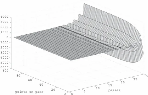
Here r(α)=1.4876 and this process is asymptotically unstable. Moreover, attempts to design a control law for asymptotic stability by the direct route failed because the required LMI cannot be solved due to its large dimension.
To commence the successive stabilization algorithm, setα1 =10 and h=10. Then
Step 1 does not provide the required stabilizing control law but Step 2 is successful and yields the stabilizing control law matrices as
K2=K12K22,
K21=−0.1569−0.1211−0.2795 0.2016 0.1442 0.0037 0.0277 0.0091 0.1013−0.0912,
where the superscript here denotes the iteration number. To apply the above control law for the wholeαextend it by 01×80(i.e. K=
K2 0) and hence˜α =α+K.
The spectral radius of subsequent matrices˜α(the matrix to whichαis mapped to under the control action) during these iterations are given in the following table
Iteration number r(˜α)
0 1.4876
1 1.6738
2 0.8379
Here asymptotic stability for the controlled process is achieved after two iterations. Note also that when the direct route was attempted, the LMI involved was found to be unsolvable numerically.
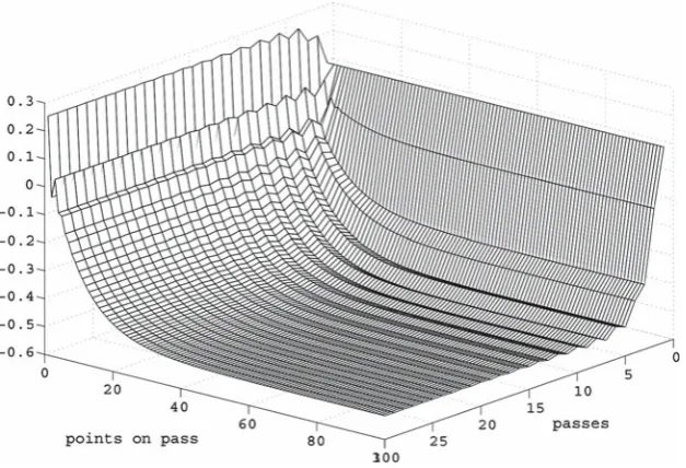
Figures2and3below show the free evolution (i.e. U(l) = 0, l= 0, 1,. . .) with-out and with the control law applied respectively and boundary conditions xk(0)=
1.8 −1.08
, k=1, 2,. . .and y0(p)=0.1, 0≤p≤99.
7 Conclusions
Control law design for discrete linear repetitive processes can involve the need to compute with extremely large dimensioned matrices and one of the major contri-butions of this paper is on the development of methods to avoid this problem. The first set of results relate to the use of preliminary control law action to completely decouple the effects of the current pas state and/or the previous pass profile vectors from the onward evolution of the process dynamics, with consequent simplifications in terms of control law design.
[image:20.439.50.360.400.598.2]Fig. 3 The controlled process pass profile sequence
The second set of results relate to the control of a new model for discrete linear repetitive processes to include a term missing from the currently used model but which could arise in applications, i.e. it is needed to capture the essential dynamics to be con-trolled. As a result, control law design algorithms based on, e.g., LMI methods may well encounter serious numerical difficulties and, moreover, the decoupling results developed in the first part of this paper only work in very restrictive special cases. To overcome these difficulties, a new stabilization procedure has been developed where the control law is designed by an iterative procedure and as the examples (and, in particular, Example 2) given, illustrate it can be applied to cases where very large dimensioned matrices arise. Further development, e.g. by using parallel/array process-ing, should allow for even larger examples well outside the range of most examples encountered and hence give a general and reliable design methodology. Finally, note that some of the LMI based results here are sufficient but not necessary and hence there is a degree of conservativeness associated with them. However, they are design algorithms which can be computed (as the examples here demonstrate) and, given the absence/computational intractability of necessary and sufficient conditions based on 2D polynomials, provide an applications oriented route forward.
References
Cichy, B., Galkowski, K., Kummert, A., & Rogers, E. (2005). Control of discrete linear repetitive processes with variable parameter uncertainty. In Proceedings of the second international
confer-ence on informatics in control, automation and robotics—ICINCO 2005, Barcelona, Spain, vol. 3,
pp. 37–42, CDROM.
Edwards, J. B. (1974). Stability problems in the control of multipass processes. Proceedings of The
Institution of Electrical Engineers, 121(11), 1425–1431.
[image:21.439.48.362.55.269.2]Galkowski, K., Paszke, W., Sulikowski, B., Rogers, E., & Owens, D. H. (2003). LMI based stability analysis and robust controller design for discrete linear repetitive processes. International Journal
of Robust and Nonlinear Control, 13(13), 1195–1211.
Galkowski, K., Rogers, E., & Owens, D. H. (1998). Matrix rank based conditions for reachability/con-trollability of discrete linear repetitive processes. Linear Algebra and its Applications, 275–276, 201–224.
Galkowski, K., Rogers, E., Xu, S., Lam, J., & Owens, D. H. (2002). LMIs—a fundamental tool in anal-ysis and controller design for discrete linear repetitive processes. IEEE Transactions on Circuits
and Systems I: Fundamental Theory and Applications, 49(6), 768–778.
Kurek, J. E., & Zaremba, M. B. (1993). Iterative learning control synthesis based on 2-D system theory.
IEEE Transactions on Automatic Control, 38, 121–125
Owens, D. H., & Rogers, E. (1999). Stability analysis for a class of 2D continuous-discrete linear systems with dynamic boundary conditions. Systems and Control Letters, 37, 55-60.
Owens, D. H., Amann, N., Rogers, E., & French, M. (2000) Analysis of linear iterative learning con-trol schemes — a 2D systems/repetitive processes approach. Multidimensional Systems and Signal
Processing, 11, 125–177
Peaucelle, D., Arzelier, D., Bachelier, O., & Bernussou, J. (2000). A new robust D-stability condition for polytopic uncertainty. Systems and Control Letters, 40, 21–30.
Roberts, P. D. (2002). Two-dimensional analysis of an iterative nonlinear optimal control algorithm.
IEEE Transactions on Circuits and Systems I: Fundamental Theory and Applications, 49(6), 872–
878.
Roesser, R. P. (1975). A discrete state-space model for linear image processing. IEEE Transactions
on Automatic Control, 20, 1–10.
Rogers, E., & Owens, D. H. (1992). Stability analysis for linear repetitive processes. Springer-Verlag Lecture Notes in Control and Information Sciences Series, Vol. 175, Berlin.
Rogers, E., Galkowski, K., Gramacki, A., Gramacki, J., & Owens, D. H. (2002). Stability and control-lability of a class of 2D linear systems with dynamic boundary conditions. IEEE Transactions on
Circuits and Systems I: Fundamental Theory and Applications, 49(2), 181–195
Sulikowski, B., Galkowski, K., Rogers, E., & Owens, D. H. (2005). Control and disturbance rejection for discrete linear repetitive processes. Multidimensional Systems and Signal Processing, 16(2), 199–216.
Bartlomiej Sulikowski received the Ph.D. degree from the
conferences: ACC, ECC, CCA, MTNS, NDS). Recently he published the book entitled “Computa-tional aspects in analysis and synthesis of repetitive processes” (University of Zielona Góra Press, 2006) summarizing his research so far. He has been a reviewer for known international conferences (e.g. CDC-ECC 2005, IFAC 2005). Furthermore, has was a member of the organizing committee of the 4th International Workshop on Multidimensional (nD) Systems, Wuppertal, Germany (July 11-14, 2005). Mr. Sulikowski’s teaching interests include Computer Networks (he’s the certified CISCO CCNA instructor), Numerical Methods and Basics of Computer Programming.
Krzysztof Gałkowski received the M.S., Ph.D. and Habilitation
(D.Sc.) degrees in electronics/automatic control from Technical University of Wrocław, Poland in 1972, 1977 and 1994 respec-tively. In October 1996 he joined the Technical University of Zielona Góra (now the University of Zielona Góra), Poland where he holds the professor position, and he is a visitng profes-sor in the School of Electronics and Computer Science, Univer-sity of Southampton, UK. In 2002, he was awarded the degree “Professor of Technical Science” the highest scientific degree in Poland. He is an associate editor of Int. J. of Multidimensional Systems and Signal Processing, International Journal of Con-trol and Int. J. of Applied Mathematics and Computer Science. He has coorganised 4 International Workshops NDS 1998 -Lagov, Poland, NDS 2000 - Czocha Castle - Poland, the third as a Symposium within MTNS 2002 in Notre Dame IN, US, and the last one NDS 2005 in Wuppertal, Germany. In 2007 NDS 2007 is organized in Aveiro, Portugal. His research interests include multidimensional (nD) systems and repetitve processes - theory and applications, control and related numerical and symbolic algebra methods. He is an author/editor of four monographs/books and about 60 papers in peer reiviewed journals and over 100 in the proceedings of international conferences. He leads an active group of young researchers in the nD systems area with strong international co-operation with the Universities of Southampton/for which he is awarded the official position of Visiting Professor at The School of Electronics and Computer Science/and Sheffield UK; the universities of Wuppertal, Erlangen-Nurnberg, Magdeburg, Germany; University of Hong Kong, University of Poitiers, IRIA, Sophia Antipolis, France. He is spending (spent) the academic year 2006-07 (2004/05) as a guest professor in The University of Wuppertal, Germany. In 2004, he obtained a Siemens Award for his research contributions.
Professor David Owens has been the Head of the
Control Council from 1999-2002 representing the interests of the UK Professional Institutions within IFAC. He has served on the Health and Safety Commission’s Nuclear Safety Advisory Committee (1995-2006) and has been an independent member of British Energy’s Training Standards and Ac-creditation Board. He is an Editor of an Institute of Mathematics and Its Applications International Journal, is an Associate Editor of several other journals and regularly contributes to international activities through conference organisation, seminars and invited lectures and committees of the In-ternational Federation of Automatic Control (IFAC).
Eric Rogers was born in 1956 near Dungannon in Northern