Computational intelligence applications to crisis management in power systems

Computational Intelligence Applications to

Crisis Management in Power Systems

Michael Negnevitsky

Centre for Renewable Energy and Power Systems

University of Tasmania

Private Bag 65 Hobart

Australia

[email protected]

Abstract—In emergency and abnormal conditions, a power system operator has to deal with a large amount of data and apply most appropriate remedial actions. However, due to emotional and psychological stress, an operator may not be able to adequately respond to critical conditions and make correct decisions. Mistakes can damage very expensive power system equipment or worse lead to major emergencies and catastrophic situations. Intelligent systems can play an advisory role suggesting the necessary actions, which should be taken to deal with a given emergency or abnormal condition as well as identifying failures of protection systems and circuit breakers. This paper outlines some experience obtained at the School of Engineering of the University of Tasmania in developing intelligent systems for power systems security. An expert system for clearing overloads applies the network sensitivity factors to determine appropriate actions, which include generation rescheduling, network reconfiguration and load shedding. An expert system for voltage control is developed and used for detecting voltage violations and providing a set of effective control actions to solve voltage problems in real-time. An artificial neural network is used to identify multiple failures of protection relays and circuit breakers. This system uses information received from protection systems in the form of alarms and is able to deal with incomplete and distorted data.

Keywords—-computational intelligence, power system, emergency condition, crisis management

I. INTRODUCTION

Computational intelligence can be considered as a successor of artificial intelligence [1-3]. It uses advanced heuristic search algorithms, artificial neural networks, the theory of fuzzy sets and evolutionary computation. Computational intelligence also employs such techniques as swarm intelligence, chaos theory, artificial immune systems, wavelet analysis, etc.

Since the early 1990s, computational intelligence techniques have been successfully applied in power systems [4-7]. Applications related to power system security are of particular interest in this paper.

Power system security includes measures which intend to keep the system in an operating condition when one or even a few components fail to operate. For example, a generating unit may fail but the remaining units of the system can increase power output to make up the deficit, and thus prevent the load shedding. Similarly, a power

transmission line may be damaged and switched-off by the power system protection but the remaining transmission lines can take the increased load.

In order to prevent a power system from collapse, its elements are operated within certain constraints and protected by automatic devices that cause equipment to be taken off if those constraints are violated. However, due to some failures, equipment may still be left in the operating state with constraints violated. Such conditions may lead in turn to switching-off other equipment out of service and if this process continues, large parts or even the entire system can collapse completely.

A major emergency in a power system might start with opening-off a single line as a result of a short-circuit. The remaining transmission system takes up the power that was flowing on that line. However, if even one of the remaining lines is now overloaded, it also may open due to an operation of the protection system, and thus an additional load is imposed on the remaining network. Moreover, a certain transmission line outage can cause some serious voltage problems as well. Therefore, power system operators are required to take immediate actions to avoid a further deterioration of the situation.

In emergency and abnormal conditions, a power system operator has to deal with a large amount of data and apply the most appropriate remedial actions. However, due to emotional and psychological stress, an operator may not be able to adequately respond to critical conditions and make correct decisions. Moreover, in emergency conditions, a vital decision must often be taken in a matter of minutes, sometimes even seconds. Mistakes can damage very expensive power system equipment or worse lead to the major emergencies and even catastrophic events. There is no time to examine advantages and disadvantages of different approaches to the restoration process and look into long columns of results. Nevertheless, an operator must respond to an emergency and only his or her experience can help to find a right decision. Clearly, there is a strong need for an aid (or decision support system) formalizing the operator’s knowledge.

II. BA S I C S O F PO W E R SY S T E M AN A L Y S I S Modern power control centers are equipped with

Supervisory Control And Data Acquisition (SCADA) systems gathering data on-line. SCADA systems enable a power system operator to apply real-time methods for power system analysis. Power operators have substantial experience in utilizing optimal power flows, state estimation, on-line security estimation and other software packages. The conventional methods employed for power system analysis rely on mathematical models and sophisticated programming techniques. However, the complexity and size of modern power systems such that complete computational solutions usually cannot be obtained in a timely fashion, and thus cannot be used in emergency conditions for decision support.

Therefore, an alternative method called the decoupled

load flow [8] is often used in emergency conditions. This method improves a computational efficiency and reduces computer storage requirements. It is reliable in solving difficult cases for large-scale power transmission systems. The major principles of the decoupled approach are based on two general rules:

• Real power flow P between two busses connected

through a power transmission line is primarily affected by the change in voltage angle δ between these busses.

• Reactive power flow Q between two busses connected

through a power transmission line is primarily affected

by the change in the voltage magnitude ⏐V⏐ at these

busses.

This approach makes it possible to develop intelligent systems for real-time applications.

III. IN T E L L I G E N T SY S T E M F O R CL E A R I N G OV E R L O A D S

A. Background

An accurate determination of permissible overloading durations for power system equipment allows operators a greater flexibility in decision making and in choosing suitable remedial actions. From an operator point of view, the most hazardous overloads are these which occur on large system transformers connecting the various voltage level networks, and on the tie power transmission lines connecting different power subsystems. Therefore, it is vital to examine factors setting limits on the overloading time of these elements.

Short-term loading capabilities of transformers depend on the ambient air temperature and the loading time. When the load increases the transformer temperature will rise and the ageing of insulating materials accelerates. Ageing sets certain limits to the loading capability of a transformer. Operating conditions at the rated power and ambient air

temperature of +20°C are considered normal. In such

cases, insulating materials will age at a normal speed and a proper maintenance can be provided. In practice, however, the load and temperature can vary according to the power demand and weather conditions. If part of the operating time the transformer loading is lower than its continuous loading capacity it can be loaded more at the other times

such that the ageing remains normal during the whole period (for example, during a 24-hour period). Therefore, permissible time for clearing transformer overloads should take into account the previous loading of the transformer or its loading history.

For transmission lines, both the power limit and the permissible duration of an overload in most cases are governed by the conductor temperature increase. On the other hand, the conductor operating temperature is limited by the conductor ground clearance. As shown in [9, 10], the loading capacity or thermal rating of a conductor can be described as a function of its temperature, ambient temperature, wind velocity, elevation, ground reflection and solar radiation. In a power transmission system, line currents during and following a system disturbance may reach values above of the steady-state thermal ratings of power lines. Such conditions may be safe for a period of up to 30 minutes. This time can be used to perform the generation rescheduling or load shedding in order to clear or at least reduce overloading. Therefore, it is necessary to determine how long a conductor can carry an overload without exceeding its maximum permissible operating temperature. This problem can be solved by employing intelligent knowledge based systems, e.g. [11].

B. Loading Capability Assessment of a Transmission Line

A heuristic nature of the short-time loading capability assessment of power transmission lines enables us to use an expert system approach. The rule-based expert system includes the basic components shown in Fig. 1.

Inference Engine Knowledge Base

(IF-THEN Rules)

Database

(Conductor Data)

External Interface

User Interface

User

Explanation Facilities

Figure 1. Expert system for the loading capability assessment.

The knowledge base contains the domain specific

knowledge in the form of IF - THEN rules. The database

includes all relevant data (conductor diameter, conductor resistance, conductor unit weight, specific heat, etc.) for various types of conductors. The data is represented in the form of a spreadsheet. The inference engine carries out the reasoning whereby the expert system reaches a solution. It links the rules given in the knowledge base and associated conditions input by the user with data provided in the

database. The explanation facilities enable the user to

query the system “How” a particular solution has been

reached. The user interface is the means of communication

between a user seeking a solution to the problem and an

expert system. The external interface allows the expert

the quantities of heat and adjusting the resistance for temperature changes.

The complete knowledge base consists of 43 rules. Details of these rules can be found in [12]. The expert system was evaluated against the site tests for both indoor and outdoor conditions. A comparison with actual test results demonstrates that the expert system represents an accurate model of the actual physical events.

Fig. 2 displays an example of the expert system query screen.

A practical application of the expert system is demonstrated on a power system of Hydro Tasmania shown in Fig. 3. The example described below examines the winter night loading conditions.

Following the outage of the Palmerston - Liapootah 220 kV transmission line, the current on the Palmerston - Waddamana transmission line increases from 182 to 623 A (196% of the steady state thermal rating). The temperature-time characteristic and short-time ratings evaluated by the expert system are shown in Figs 4 and 5. It can be seen that the conductor temperature increases

from 20°C (initial temperature) to 43°C (the maximum

permissible temperature limited by the conductor ground clearance) in 1 minute. Therefore, this overload should be allowed for 1 minute only. This conclusion is displayed on the screen as shown in Fig. 6.

This question is asked to assign the specific heat value for the conductor. Consider, for example, the cpecific heat at 20 C of the following conductors:

Aluminium = 900 J/Kg . C degree

Copper = 385

Steel = 431

What is the conductor type?

Aluminium Copper ACSR

F keys: 1 Help 2 Quit 3 Why? 5 Volunteer 6 Backup 7 Expand 8 Review

Figure 2. The expert system query screen.

Sheffield

Palmerston

Liapootah

Waddamana Palmerston 220 kV

110 kV Norwood

Trevallyn

West-Coast

Mersey-Foth

Derby/Scott. 285 MW

435 MW

40 MW

290.1 + j11.8 (290.4)

118.1 - j13.1 (118.8)

110.4 - j13.1 (111.2)

11.5 + j3.4 56.1 + j20.3

22.5 +j 7.4 8.8 +j 2.2

623 A 583 A

outage

Southern area G

G

G

Figure 3. The HEC system: a case study.

43

Conditions:

wind = 0.5 m/s, elevation = 760 m ambient = 10 *C, emissivity = 0.915 initial current = 182 A

initial temp = 20 *C final current = 623 A final temp = 168 *C

1

Figure 4. Temperature-time characteristics of the Waddamana-Palmerston transmission line.

623 A

Conditions:

wind = 0.5 m/s, elevation = 760 m ambient = 10 *C, emissivity = 0.915 initial current = 182 A

initial temp = 20 *C final current = 623 A final temp = 43 *C

Figure 5. Short time ratings for the Waddamana-Palmerston transmission line.

EXPERT SYSTEM

Short-Time Thermal Rating of Transmission Lines Conclusion

Conductor type: 19/ .083" Copper

Type any key to see the next screen

LEONARDO (c)1986-1990 Creative Logic Ltd. Knowledge Base: CONDUCTOR

Operating condition:

elevation (m): 760 wind (m/s): 0.5 Conductor temperature:

initial (*C): 20 Conductor current:

initial (A): 182

Permissible overload duration (min.): Steady state thermal rating (A):

final (A): 623 emissivity: 0.915 ambient (*C): 10

final (*C): 43

317 1.00

Figure 6. Conclusion screen.

C. Sensitivity Factors

Gj i ij

P S

Δ Δ =

α (1)

where ΔS_i is the change in power flow on element i when a

change in generation, ΔP_Gj, occurs at bus j. If it is

assumed that all other generators remain fixed, then the α_ij factor represents the sensitivity of the power flow on element i to a change in generation at bus j.

The network reconfiguration factors are used in a similar manner. The line outage distribution factor has the following meaning:

0 ,

k i k i

S S

Δ =

β (2)

where β_i,k is the line outage distribution factor when

monitoring element i after an outage on line k; ΔS_i is the change in power flow on element i; S_k0 is the original flow on line k before it was opened.

The load shedding factors can be obtained as:

Ln i ij

P S

Δ Δ =

γ (3)

where ΔS_i is the change in power flow on element i when a change in load, ΔP_Ln, occurs at bus n.

The overload clearing is a subject to the following security constraints:

max min

Gj Gj Gj

Gj P P P

P ≤ +Δ ≤ (4)

max 0

max

i i i

i S S S

S ≤ +Δ ≤

− (5)

max

Ln Ln

Ln P P

P −Δ ≥ (6)

max min

j j

j V V

V ≤ ≤ (7)

where P_Gjmax, P_Gjmin and P_Gj are the maximum and

minimum limits and operating value of the generator output in MW at bus j, respectively; S_i0, ΔS_i and S_imax are

the original MVA flow on line i, change in MVA flow on

the same line after an outage of line k and the long-term

rating (or emergency rating) of line i, respectively (the

minus sign indicates that the line flow can be either positive or negative); P_Lnmin and P_Ln are the guaranteed

minimum load supply and the original load at bus n,

respectively; V_jmax, V_jmin and V_j are the maximum and

minimum voltage limits and the actual voltage at bus j,

respectively.

In order to find the most effective corrective actions for a given overload, the sensitivity tree method is used. The tree provides relationships between an overloaded power line load and available controllers.

D. Knowledge Base and Database

Any overload can be classified using answers to the following questions [13]:

1. What is the type of plant? 2. What is the overload duration?

3. What is the overload permissible duration?

4. What are the means available for clearing the overload? 5. What is the action to be applied first?

This provides the basis on which the database and the knowledge base are organized. The expert system for clearing overloads uses the following data:

• The upper load limits (short-term rating) for each

supervised element.

• The permissible overload duration for each supervised

element as a function of the load. The permissible time for clearing an overload can be obtained using the data provided in loading guides [14], calculated, e.g. [9, 15, 16], or employing intelligent systems as it was discussed above.

• The upper and lower limits for each power station (or,

if required, for each generator).

• The long-term ratings (emergency ratings) for each

power transmission line.

• The guaranteed minimum load supply (or the highest

priority load level) at each bus.

• The sensitivity factors for each supervised element and

controller, and also the execution time for each controller.

E. Production Rules

The expert system applies the following heuristic rules specified in [13]:

Rule 1:

IF the real power flow on element i is more than its short-term rating, THEN element i is overloaded.

Rule 2:

IF element i is overloaded, THEN include element i in the list of overloaded elements.

Rule 3:

IF element i is in the list of overloaded elements, THEN

determine permissible overload duration t_i for element i.

Rule 4:

IF permissible overload duration t_i is the lowest over all elements in the list of overloaded elements, THEN calculate the sensitivity factors (generator shift, network reconfiguration and load shedding).

Rule 5:

IF the generator shift list is not empty, THEN select the most effective controller AND check its limits AND calculate the overload relief on element i.

Rule 6:

IF the overload relief caused by the selected controller is

less than the overload magnitude of element i AND the

controller execution time is less than permissible overload

duration t_i, THEN include the controller in the list of

feasible actions.

Rule 7:

Rule 8:

IF element i is still overloaded AND the network

reconfiguration list is not empty, THEN select the most effective controller AND check long-term rating violations on the other elements after the controller is applied AND calculate the overload relief on element i.

Rule 9:

IF the selected controller does not cause long-term rating violations on the other elements AND the overload relief is

less than the overload magnitude of element i AND the

controller execution time is less than permissible overload

duration t_i, THEN include the controller in the list of

feasible actions.

Rule 10:

IF element i is still overloaded, THEN select next available controller on the network reconfiguration list until all controllers are taken.

Rule 11:

IF element i is still overloaded AND the load shedding list is not empty, THEN select the most effective bus (a bus where the load shedding causes the most significant effect on the overload relief of element i) AND calculate the load shedding required to clear the overload on element i.

Rule 12:

IF the required load shedding is less than the load at the selected bus minus the guaranteed minimum load supply AND the shedding execution time is less than permissible

overload duration t_i, THEN include the required load

shedding at the selected bus in the list of feasible actions.

Rule 13:

IF the required load shedding is greater than the load at the selected bus minus the guaranteed minimum load supply AND the shedding execution time is less than permissible

overload duration t_i, THEN include the allowable load

shedding at the selected bus in the list of feasible actions.

Rule 14:

IF element i is still overloaded, THEN select next bus on

the shedding list until the overload on element i is cleared.

Rule 15:

IF the overload on element i is cleared, THEN take next

element on the list of the overloaded elements until the list becomes empty.

F. Case Study

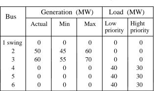
A six-bus system shown in Fig. 7 is used to demonstrate the performance of the developed expert system. Table 1 represents bus data of the system.

1 2 4 6 5 3 G G G

Figure 7. Six-bus power system.

Table 1: Bus data of the system.

Generation (MW)

1 swing 2 3 4 5 6 Bus

Actual Min Max Low

Load (MW)

0 50 60 0 0 0 0 45 55 0 0 0 0 60 70 0 0 0 0 40 40 0 0 40 0 30 30 0 0 30 priority Hight priority

Table 2 shows line limits and initial MVA flows on the lines. Line 2-6 is overloaded in the initial state. Columns 4 and 5 represent flows after corrective actions suggested by the expert system have been applied.

Line flows are determined using ac load flow and according to the recommendations made by the expert system.

Table 3 shows available actions which may be used to clear the overload on line 2-6 and corresponding sensitivity factors. Some actions are not applicable due to security constraints. For example, a disconnection of line 1-4 leads to overloads on lines 1-2, 1-5 and 2-5 and a voltage violation on bus 4.

Table 2: Case studies.

Line Line limit

50.0 65.0 50.0 25.0 65.0 35.0 25.0 35.0 85.0 25.0 25.0 32.6 48.0 37.3 12.6 56.7 21.9 29.4 30.1 75.1 6.4 9.7 0.0 60.6 45.7 11.6 55.1 19.7 25.0 29.8 76.6 5.9 10.8 27.7 45.2 33.7 11.5 57.5 21.4 25.0 31.2 74.4 5.4 9.2 Initial flow Case 1

1 - 2 1 - 4 1 - 5 2 - 3 2 - 4 2 - 5 2 - 6 3 - 5 3 - 6 4 - 5 5 - 6

Case 2

Table 3: Available actions and sensitivity factors.

Action Bus Sensitivity Factor

Generation Increase Generation Increase Load Shedding Load Shedding Load Shedding Line Disconnection Line Disconnection Line Disconnection Line Disconnection Line Disconnection Line Disconnection Line Disconnection Line Disconnection Line Disconnection Line Disconnection 2 3 4 5 6 1 - 2 1 - 4 1 - 5 2 - 3 2 - 4 2 - 5 3 - 5 3 - 6 4 - 5 5 - 6

-0.0514 not applicable 0.1824 -0.0148 0.1093 0.3484 0.0745 not applicable not applicable not applicable not applicable -0.0977 0.0297 -0.1287 -0.0024

According to recommendations provided by the expert system, the following actions are to be applied (Case 1):

• Bus 2, decrease generation on 5 MW;

• Bus 3, increase generation on 10 MW;

• Line 1-2, switch off.

• Bus 2, decrease generation on 5 MW;

• Bus 3, increase generation on 10 MW;

• Bus 6, shed load by 6.5 MW.

IV. EX P E R T SY S T E M F O R VO L T A G E CO N T R O L

A. Problem Statement and Sensitivity Tree Method

The main objective of voltage control is to maintain power system voltages within specified limits under various loading conditions and changes in the transmission network. Classical analytical methods based on different optimization techniques intend to minimize system losses and improve voltage profiles. However, most of these methods are too complex, provide analytical solutions only, and cannot recommend appropriate control actions required to overcome voltage violations in a given emergency condition.

In order to improve the computational performance, a reduced system can be built using the subsystem reduction and equivalencing techniques described in [17]. The reduced system consists of an internal “three-tier” subsystem that introduces the voltage problem area, and the external subsystem that represents the rest of the power system. This approach allows to minimize the system size and eliminate the less effective voltage controllers. Therefore, voltage magnitudes can be predominantly controlled by the reactive power injections into the internal subsystem. An expert system technique can be used to provide a set of practically effective control actions to solve a given voltage problem in real-time.

Voltage controllers can change their values either continuously or in steps, they are not equally effective and adjustments required from an individual controller are different under different power system conditions. The sensitivity tree method is used to find the effective order of control actions to be applied. It provides the relationship between bus voltages and the controller settings. A sensitivity matrix which relates the changes in the

controlled variables, ΔX, to the changes in the controller

settings, ΔU, may be described as suggested in [18]:

[ΔX] = [S] [ΔU] (8)

where matrix [S] provides sensitivity factors between settings of the controllers and bus voltages. Voltage at any bus in the system can be adjusted by several different controllers. On the other hand, a change in any controller setting results in voltage changes on several buses.

B. Database and Knowledge Base

The developed voltage control expert system interacts with the power flow analysis package, network sensitivity analysis and other external programs and databases. The expert system uses the following data:

• Upper and lower limits of voltage at each bus;

• Upper and lower limits of each controller;

• Sensitivity factors for each load bus and each

controller.

When a bus voltage exceeds its specified limits, either high or low, a power system operator can adjust transformer taps, change generator bus voltages and switch capacitor banks and reactors on or off.

The voltage control expert system performs the following tasks:

1. Determine the problem area and build an internal

“three-tier” subsystem.

2. Calculate the network sensitivity factors and build the

sensitivity tree.

3. Identify all buses with abnormal voltages.

4. Select the bus with the maximum level of voltage

violation.

5. Select the most effective controller, estimate controller

effect and check security constraints.

6. If security constraints are not violated then implement

the controller selected. If security constraints are violated then proceed to the next task.

7. If the voltage problem still exists then select the next

available controller until all controllers are taken.

8. If the voltage on the maximum violated bus has become

normal then take the next bus with the maximum abnormal voltage and repeat the procedures.

Some of the rules implemented in the knowledge base are listed below:

Rule 1:

IF voltage on bus i is below the voltage limit THEN bus i

is a low voltage problem bus.

Rule 2:

IF bus i is a low voltage problem bus THEN include bus i

in the low voltage problem bus list AND arrange buses in the voltage ascending order.

Rule 3:

If all voltage problem buses are determined THEN calculate the sensitivity factors.

Rule 4:

IF the controller list for a low voltage problem bus is not empty THEN select the most effective controller.

Detailed description of the expert system developed can be found in [19, 20].

C. Performance Evaluation

The purpose of evaluation is to validate the knowledge incorporated in the production rules, and to compare the expert system performance with a conventional approach. Results are demonstrated on the modified IEEE 30-bus test system shown in Fig. 8. The most severe case is an outage of transformer T1 connected between buses 27 and 28.

Fig. 9 shows the one-line diagram of the reduced system (equivalent system) for the outage of transformer T1. In this system, all the control measures in the external areas are retained. The “three-tier” internal subsystem incorporates the following buses:

• First tiers: 27, 28.

• Second tiers: 6, 8, 25, 29, 30. • Third tiers: 2, 4, 7, 9, 10, 24, 26.

2 5 6 4 12 11 14 15 23 18 19 10 G 1 G 3 G 13 31 24 20 16 17 22 21 7 25 26 8 27 28 29 30 9 32 33 34 T1 G G G

Figure 8. The modified IEEE 30-bus system.

2 5 6 4 12 11 14 15 10 G 1 G G 3 G G 13 31 24 7 25 26 8 G 27 28 29 30 9 32 33

1st tier buses 2nd tier buses

external buses 3rd tier buses

fictitious lines

T1

Figure 9. The equivalent IEEE 30-bus power system.

Recommendations given by the expert system on voltage control actions to be taken under the outage of transformer T1 are shown in Fig. 10.

Table 4: Bus voltages and optimal control settings.

Remarks Load voltages V3 V4 V6 V7 V9 V10 V12 V14 V15 V16 V17 V18 V19 V20 V21 V22 V23 V24 V25 V26 V27 V28

1.026 1.014 1.020 1.003 1.016 0.999 1.005 0.995 0.999 1.059 0.955 1.041 0.972 1.051 0.950 1.023 *0.943 1.032 0.957 1.040 0.950 1.035 *0.934 1.023 *0.932 1.021 *0.937 1.025 *0.934 1.026 *0.933 1.025 *0.915 1.013 *0.888 0.998 *0.818 0.974 *0.796 0.955 *0.789 0.971 1.018 1.001

1.026 1.014 1.020 1.003 1.016 0.999 1.005 0.995 0.999 1.059 0.955 1.041 0.972 1.051 *0.950 1.020 *0.943 1.031

*0.887 0.998 *0.818 0.973 *0.795 0.955 *0.788 0.970 1.018 1.001 Full system Equivalent Initial Final Initial Final

Remarks Load voltages V29 V30 V31 V32 V33 V34 Gen. setting V1 V2 V5 V8 V11 V13 Trans. setting

N:3 - 31 N:4 - 12 N:6 - 9 N:6 - 10 N:14 - 32 N:15 - 33 N:27 - 28

*0.763 0.955 *0.747 0.950 0.975 1.027 0.975 1.027 0.982 0.960 0.962 0.978

1.050 1.060 1.045 1.045 1.010 1.010 1.025 1.025 1.050 1.050 1.050 1.050 1.069 1.000 1.032 0.901 0.978 0.903 1.069 0.900 0.950 0.950 0.950 1.094 --- outage ---

*0.762 0.954 *0.746 0.950 0.975 1.027 0.975 1.027 0.982 0.960

1.050 1.060 1.045 1.045 1.010 1.010 1.025 1.025 1.050 1.050 1.050 1.050 1.069 1.000 1.032 0.901 0.978 0.903 1.069 0.900 0.950 0.950 0.950 1.094 outage ---Full system Equivalent Initial Final Initial Final

Note: ( * ) bus with voltage constraints violated.

Task 2: Detect voltage violations

* number of voltage violations: 13

* the lowest voltage occurs at bus: 30 { V(30) = 0.747 p.u. }

Task 3: Correct voltage violations Task 1: Calculate the sensitivity factors

Action 1: select controller: transformer 6 - 9

adjust its setting: 0.978 0.903 { V(30) = 0.769 p.u. } Action 2: select controller: transformer 6 - 10

adjust its setting: 1.069 0.900 { V(30) = 0.810 p.u. } Action 3: select controller: transformer 4 - 12

adjust its setting: 1.032 0.901 { V(30) = 0.839 p.u. } Action 4: select controller: generator 1

adjust its setting: 1.050 1.060 { V(30) = 0.842 p.u. } Action 5: select controller: transformer 3 - 31

adjust its setting: 1.069 1.000 { V(30) = 0.846 p.u. } Action 6: select controller: transformer 15 - 33

adjust its setting: 0.950 1.094 { V(30) = 0.850 p.u. }

** This voltage violation cannot be corrected by the available controllers ** VAR compensation is required

Figure 10. Voltage control action screen.

The expert system performs well and provides correct decisions. The new approach offers the following advantages:

• The computational performance can be improved by

reducing the size of power systems.

• The use of the expert system, steady state equivalent

network and power system reduction techniques meets both speed and accuracy requirements for detecting and correcting voltage violations. Hence, the proposed techniques can be used for on-line voltage control applications.

• Analytical results are complemented by description of

actions and, hence, are easy to understand.

V. NEURAL NETWORK FOR ON-LINE IDENTIFICATION OF

MULTIPLE FAILURES

A. Fault Identification Problem

In complex emergency situations, failed protection relays and circuit breakers (CB) have to be identified in order to begin the power system restoration process. In fact, re-energizing defective or unprotected equipment can expand the damage and spread the problem, and it is often the cause of cascading blackouts [21].

Studies of large emergencies in power systems indicate that failures of protection relays are involved in 75% of cases [22]. An identification of faulted sections and malfunctions of protection relays and CBs requires an extensive knowledge of the behavior of protection systems during various conditions [23-27]. Due to the fact that this problem is non-linear, large-scale and often has a combinatorial nature, various artificial intelligence techniques have been explored and successfully used. In particular, expert system and neural network approaches have proved to be the most effective in dealing with this level of complexity.

complex as one needed detailed and reliable data to start with. Unfortunately, such data may not always be available. In addition, protection system analysis is time consuming and requires a complex reasoning process. During a complex emergency the number of possible situations is often enormous, which makes the operator’s job of making decisions very difficult. As a result, complex emergencies often lead to large system blackouts and serious damages to power equipment. From a practical point of view, it is also desirable to be able to analyze complex emergencies with multiple cascading failures [28].

An emergency in a power system can be represented by a set of three vectors:

F R S

E = , , (9)

where vector S includes one or more sections of a power

system where a fault occurs, vector R is a set of relays that have operated and CBs that have tripped as a result of the

fault; and vector F is a set of protection devices and CBs

that should have operated during the fault but failed to do

so. Emergency E is considered complex if vector F has

two or more elements.

Pattern P of emergency E (referred to as PE) is usually observed in a control centre; it is represented by a set of

alarms. In fact, this pattern is a mapping of vector R.

Pattern PE can also be expressed as a set of statements in the form: <Alarm name, Alarm value>. In general, the number of statements equals to the maximum number of alarms provided by the SCADA system. If the alarm has been received then its value is 1, and if the alarm has not been received then its value is 0. Pattern P of emergency E

can be represented as a binary vector:

E m E E

E _{A A A}

P = ₁ , ₂ ,..., (10)

where AiEis the value of alarm i (either 0 or 1), and m is the pattern dimension.

A perfect pattern of emergency E, POE, is a complete set of alarms (without any errors in the SCADA system) for a single pre-fault configuration of a power system. The perfect pattern is, in fact, the set of devices that have operated (POE=RE).

Corrupted pattern of emergency E, PCE, is an

incomplete and/or distorted pattern. The same emergency can, in fact, be described by a set of corrupted patterns, <PCE >. This set is called the pattern space of emergency

E, and can be defined as:

E N m E N E N E m E E E m E E E E

E A A

A A A A A A A E C P , , 2 , 1 2 , 2 , 2 2 , 1 1 , 1 , 2 1 , 1 , ... , , ... ..., , ... , , , ... , ,

= (11)

where Ai,jE is the value of alarm i (either 0 or 1) for

corrupted pattern j of emergency E, and NE is the total

number of corrupted patterns of emergency E.

The goal now is to find a set of failed protection devices and CBs - set FE- based on corrupted pattern PCE. The problem can be formulated as a pattern classification problem. In this case, an emergency situation (represented by pattern PC,jE) has to be classified into one of several possible classes, where each class corresponds to a single

combination of failed devices (vector FE). Neural

networks offer a practical approach to solving such complex pattern classification problems [3].

B. The Problem Decomposition

A single emergency may generate up to 500 different alarms. However, each section of a power system produces its own set of alarms. The maximum number of such alarms for a single section does not normally exceed 35-40. Thus, in order to reduce the problem dimensionality, a neural network should be constructed individually for each section. The solution can be expressed as following [29]:

1. Simulate the response of protection systems in the case

of two failures.

2. Form a set of all possible alarms, and a set of all relays and CBs that fail to operate.

3. Form a pattern space of an emergency and creating a

training set.

4. Construct and train a NN.

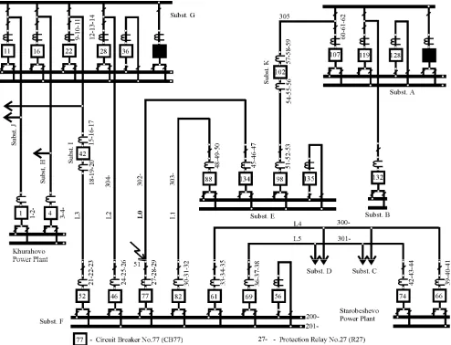
Simulation of emergency situations is demonstrated on the 110 kV power system shown in Fig. 11. It has two power plants, five substations, 10 transmission lines, and 14 buses. The protection system consists of 304 relays.

Fig. 12 represents a graph of all possible emergencies when a fault occurs on line L0. As can be seen, there are 25 possible emergencies that can be caused by this fault. There are three emergencies with a single failure (the first level of the graph) and 22 complex emergencies with two cascading failures of protection relays and/or CBs (the second level of the graph). A detailed analysis of each emergency is given in Table 5. Fig. 13 shows the NN used. It has 32 inputs and 20 outputs. The number of inputs corresponds to the number of alarms. The number of outputs corresponds to the number of devices that failed to operate – set F in Eq. (9).

C. Structure of the Neural Network Identification System

Preliminary simulations demonstrated that using only perfect patterns of emergencies in a training set leads to large recognition errors. To improve the NN performance, errors of the SCADA system are simulated by inserting a single random alarm error into a perfect pattern. Also the data loss is simulated by removing a single random alarm from a perfect pattern. As a result, a set of 5072 corrupted patterns is generated and then used to train and test the NN. To estimate a similarity between the 25 emergencies shown in Fig. 12, the Hamming distance between different

classes is calculated. The distance between classes EX and

EY representing emergencies X and Y, respectively, is

determined as [30]:

(

)

X A A

m N N E E d Y X

1 , ,

1 1

1 1 1

Figure 11. The 110 kV power system.

Table 5: Simulated emergencies.

Emergency S Operated relays and tripped CBs, (R) Failed devices, (F)

E1 L0 R27,CB77,R46,CB134 R302

E2 L0 R302,CB77,R46,R32,CB82,R47,R56,CB102 CB134

E3 L0 R302,CB134,R27,R19,CB42,R49,CB88,R13,CB28,R40,CB66,R43,CB74 CB77

E4 L0 R27,CB77,R46,R32,CB82,R47,R56,CB102 R302,CB134

E5 L0 R27,R19,CB42,R49,CB88,R13,CB28,R28,R40,CB66,R43,CB74,R46,CB134 R302,CB77

E6 L0 R302,R27,R19,CB42,R49,CB88,R13,CB28,R28,R40,CB66,R43,CB74,R46,R47,R56,CB102 CB134,CB77

E7 L0 R19,CB42,R49,CB88,R13,CB28,R28,CB77,R40,CB66,R43,CB74,R46,CB134 R302,R27

E8 L0 R27,CB77,R32,CB82,R47,CB134 R302,R46

E9 L0 R302,CB77,R32,CB82,R47,R56,CB102 CB134,R46

E10 L0 R302,CB77,R46,R47,R14,CB28,R20,CB42,R41,CB66,R44,CB74,R56,CB102 CB134,R32

E11 L0 R302,CB77,R46,R32,R47,R14,CB28,R20,CB42,R41,CB66,R44,CB74,R56,CB102 CB134,CB82

E12 L0 R302,CB77,R46,R32,CB82,R47 CB134,R56

E13 L0 R302,CB77,R46,R32,CB82,R47,R56 CB134,CB102

E14 L0 R302,CB134,R19,CB42,R49,CB88,R13,CB28,R28,R40,CB66,R43,CB74 CB77,R27

E15 L0 R302,CB134,R27,R49,CB88,R11,CB22,R13,CB28,R28,R40,CB66,R43,CB74 CB77,R19

E16 L0 R302,CB134,R27,R19,R49,CB88,R11,CB22,R13,CB28,R28,R40,CB66,R43,CB74 CB77,CB42

E17 L0 R302,CB134,R27,R19,CB42,R13,CB28,R28,R40,CB66,R43,CB74,R29,R50,CB88,R56,CB102 CB77,R49

E18 L0 R302,CB134,R27,R19,CB42,R49,R13,CB28,R28,R40,CB66,R43,CB74,R29,R50,R56,CB102 CB77,CB88

E19 L0 R302,CB134,R27,R19,CB42,R49,CB88,R28,R40,CB66,R43,CB74,R14,CB28,R29 CB77,R13

E20 L0 R302,CB134,R27,R19,CB42,R49,CB88,R13,R28,R40,CB66,R43,CB74,R104,CB16,CB36 CB77,CB28

E21 L0 R302,CB134,R27,R19,CB42,R49,CB88,R13,CB28,R40,CB66,R43,CB74 CB77,R28

E22 L0 R302,CB134,R27,R19,CB42,R49,CB88,R13,CB28,R28,R43,CB74,R29,R41,CB66 CB77,R40

E23 L0 R302,CB134,R27,R19,CB42,R49,CB88,R13,CB28,R28,R40,CB66,R29,R44,CB74 CB77,R43

E24 L0 R302,CB134,R27,R19,CB42,R49,CB88,R13,CB28,R28,R40,R43,CB74,R29,R41 CB77,CB66

Fgfgfgfggr5

Level I

Level II

Figure 12. The emergency graph for section L0.

Figure. 13. The multi-layer perceptron.

where NX is the number of corrupted patterns in class EX,

NY is the number of corrupted patterns in class EY, AXk,i is

the value (either 0 or 1) of alarm k in corrupted pattern i of emergency X, and AYk,j is the value (either 0 or 1) of alarm k in corrupted pattern j of emergency Y.

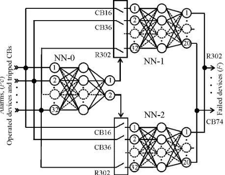
The NN-based identification system is shown in Fig. 14. Neural network NN-0 separates emergencies into two

classes. Class 1 represents emergencies with one failed

device and class 2 emergencies with two failed devices. If a pattern is classified as an emergency of class 1 then NN-1 is used. However, if a pattern is classified as an

emergency of class 2 then NN-2 is used. NN-1 and NN-2

are trained with patterns describing emergencies with one and two failures, respectively.

Figure 14. The NN-based identification system.

The entire set of 5072 corrupted patterns is randomly divided into training, test and evaluation sets. The training set includes 2536 training samples and is used for training NN-0. A training example is represented as:

E E E

j E

j E

j A A O O

A_1, , _2, , ..., _32, , ₁ , ₂ (13)

where Ai,jE is the NN input represented by the value of

alarm i (either 0 or 1) for corrupted pattern j of emergency

E; O1E and O2E are the NN desired outputs. If O1E is 1 and

O2E is 0, then E is an emergency with a single failed

device. If O1E is 0 and O2E is 1, then E is a complex emergency with two failed devices.

To train NN-1 and NN-2 the following data sets were created:

E E E E

j E

j E

j A A F F F

A_1, , _2, , ..., _32, , ₁ , ₂ ,..., ₂₀ (14)

where FiE is the desired value of NN output i for

emergency E. If FiE is 1, then device i fails to operate during emergency E, but if FiE is 0, then device i operates successfully. An optimal number of hidden neurons is determined based on the analysis of the network performance. Results are given in Table 6.

Table 6: Evaluation results

Neural Networks NN-0 NN-1 NN-2

Input 32 32 32

Hidden 7 13 15

Output 2 20 20

Training 2536 2132 4050

Test 1268 1066 2025

Evaluation 1268 1066 2025

Training 0.0009 0.0009 0.0210

Test 0.0010 0.0012 0.0211

Evaluation 0.0023 0.0013 0.0220

Epoch 600 250 1000

Neu

ron

s

Ex

am

p

les

MS

E

D. Case Studies

For emergencies with two failures, the NN-based identification system can produce three possible outcomes: correct recognition, inadequate recognition and incorrect recognition. In the case studies presented here, emergency patterns are corrupted by both distorted (one alarm is false) and incomplete (one alarm is missing) signals.

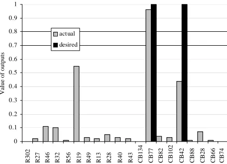
• Case 1: Correct recognition.

This case is illustrated in Fig. 15. Emergency E18

occurs as a result of a short circuit on transmission line L0 (near Substation F, point 51). The primary transmission line protection R302 operates and sends tripping signals to breakers CB77 and CB134. Breaker CB134 trips while the other breaker, CB77, fails to operate. Substation F is then de-energized by tripping CBs on adjacent substations.

substation E fails to trip. As a result of this failure, the 3rd zone of distance relay R56 on substation K causes breaker CB102 to open. It results in de-energizing both substations,

F and E. All devices that operated in emergency E18 are

shown in Table 5.

R27 R46 R32 R56 R19 R49 R13 R28 R40 R43 CB134 CB77 CB82 CB102 CB42 CB88 CB28 CB66 CB74

R302

0 0.1 0.2 0.3 0.4 0.5 0.6 0.7 0.8 0.9 1

Value of outputs

actual desired

Figure 15. Case 1: Correct identification.

• Case 2: Inadequate recognition.

Fig. 16 illustrates a situation when the system cannot

identify emergency E16. This emergency is caused by two

failed devices CB77 and CB42. The first device, CB77, is identified, but the second one, CB42, is not. The maximum values of the NN outputs indicate failed devices CB77 and R19. The reason for an inadequate recognition is the similarity between patterns of these two emergencies. (the

Hamming distance between classes E16 and E15 is 2.2,

which is relatively small). Thus, an operator should obtain some additional information before making the final diagnosis in this situation.

R302 R27 R46 R32 R56 R19 R49 R13 R28 R40 R43 CB134 CB77 CB82 CB102 CB42 CB88 CB28 CB66 CB74

0 0.1 0.2 0.3 0.4 0.5 0.6 0.7 0.8 0.9 1

Val

ue of

out

put

s

actual desired

Figure 16. Case 2: Inadequate identification.

• Case 3: Incorrect recognition.

The corrupted pattern of complex emergency situation

E7 cannot be recognized. This emergency is a result of a

double failure: primary protection R302 and local backup protection R27 on line L0. The corrupted pattern also includes false alarm R20 and missing alarm R49. The NN response is shown in Fig. 17.

R302 R27 R46 R32 R56 R19 R49 R13 R28 R40 R43 CB134 CB77 CB82 CB102 CB42 CB88 CB28 CB66 CB74

0 0.1 0.2 0.3 0.4 0.5 0.6 0.7 0.8 0.9 1

Va

lue

of outputs

act ual desired

Figure 17. Case 3: Incorrect identification.

VI. CONCLUSION

Prototype intelligent systems for clearing overloads, voltage control and multiple failure identification in power systems have been developed and successfully evaluated. The expert system for clearing overloads applies the network sensitivity factors to determine appropriate actions, which include generation rescheduling, network reconfiguration and load shedding. The expert system for voltage control is used for detecting voltage violations and providing recommendations for solving voltage problems in real-time. The multiple failure identification system is based on artificial neural networks. It is used to identify failures of protection relays and circuit breakers during emergency conditions. This system uses information received from protection systems in the form of alarms and is able to deal with incomplete and distorted data.

VII.RE F E R E N C E S

1. Engelbrecht, A. P. Computational Intelligence: An Introduction, Wiley & Sons, New York, 2007.

2. Poole, D, Mackworth, A. and Goebel R., Computational Intelligence: A Logical Approach, Oxford University Press, New York, 1998.

3. Negnevitsky, M., Artificial Intelligence: A Guide to Intelligent Systems, 2nd ed., Addison Wesley, Harlow, England, 2005.

4. Dillon, T. S. and Laughton M. A., Expert system applications in Power Systems, Prentice Hall International, London, 1990. 5. Tomsovic, K., “Current Status of Fuzzy Set Theory

Applications to Power Systems”, Trans. of the IEE of Japan, 1993, 113-B, (1), 2 - 6.

6. Dillon, T. S. and Niebur, D., Neural Networks Applications in Power Systems, CRL Publishing, London, 1996.

7. Lai, L. L., Intelligent System Applications in Power Systems: Evolutionary Programming and Neural Networks, Wiley & Sons, New York, 1998.

8. Stott B. and Alsac, O. “Fast Decoupled Load Flow”, IEEE Trans. on Power Apparatus and Systems, 1974, PAS-93, May/June, 859 - 869.

9. Morgan, V. T. Thermal Behavior of Electrical Conductors, Research Studies Press, John Wiley, 1991.

11. Negnevitsky, M. and Le, T. L., “Clearing Overloads in Power Transmission Systems: A Knowledge-Based Approach”, International Journal of Power and Energy Systems, 1999, 19, (2), pp. 186 - 192.

12. Le, T.L., Negnevitsky, M. and Piekutowski, M. “Expert System Application for the Loading Capability Assessment of Transmission Lines”, IEEE Trans. on Power Systems, 1995, 10, (4), pp. 1805 - 1812.

13. Negnevitsky, M., “An Expert System Application for Clearing Overloads”, International Journal of Power and Energy Systems, 1995, 15, (1), pp. 9 - 13.

14. International standard: IEC 60076-7 Loading Guide for Oil-Immersed Power Transformers, IEC, 2005.

15. Seppa, T. O., “FACTS and real time thermal rating - synergistic network technologies”, Power Engineering Society General Meeting, IEEE, June 2005, pp. 2416 - 2418. 16. Piccolo, A., Vaccaro, A. and Villacci, D., “Thermal rating

assessment of overhead lines by Affine Arithmetic”, Electric Power Systems Research, 2004, 71, (3), pp. 275 - 283. 17. Housos, E. C., et. al. “Steady state network equivalents for

power system planning applications”, IEEE Trans. on Power Systems, 1980, PAS-99, (6).

18. Hano, I., Tamura, Y. and Narita, S. “Real time control of system voltage and reactive power”, IEEE Trans. on Power Apparatus and Systems, 1969, PAS-88, (10), pp. 1544 - 1558. 19. Le, T.L., Negnevitsky, M. and Piekutowski, M. “Expert

system application for voltage control and VAR compensation”, Engineering Intelligent System, 1995, 3, (2), pp. 79-85.

20. Le, T. L. and Negnevitsky, M., “Expert System Application for Voltage and VAR Control in Power Transmission and Distribution Systems”, IEEE Trans. on Power Delivery, 1997, 12, (3), pp. 1392 - 1397.

21. Tamronglak, S., Horowitz, S. H., Phadke, A.G. and Thorp, J., “Anatomy of power system blackouts: preventive relaying strategies”, IEEE Trans. on Power Delivery, vol. 11, Apr. 1996, pp. 708 – 714.

22. Jung, J., Liu, C.-C., Hong, M., Gallanti, M., and Tornielli, G., “Multiple hypotheses and their credibility in on-line fault diagnosis”, IEEE Trans. Power Delivery, vol. 16, Jun. 2001, pp. 225 - 230.

23. Fukui, C. and Kawakami, J., “An expert system for fault section estimation using information from protective relays and circuit breakers”, IEEE Trans. Power Delivery, vol. 1, Oct. 1986, pp. 83-90.

24. Huang, Y.-C., “Fault section estimation in power systems using a novel decision support system”, IEEE Trans. Power Systems, vol. 17, May. 2002, pp. 439-444.

25. Huang, Y.-C., “Abductive reasoning network based diagnosis system for fault section estimation in power systems” IEEE Trans. Power Delivery, vol. 17, Apr. 2002, pp. 369-374. 26. C.-F. Chien, S.-L. Chen, and Y.-S. Lin, “Using Bayesian

network for fault location on distribution feeder”, IEEE Trans. Power Delivery, vol. 17, Jul. 2002, pp. 785-793. 27. Souza, J. C. S., Rodrigues, M. A. P., Schilling, M. T. and Do

Coutto Filho, M. B., “Fault location in electrical power systems using intelligent systems techniques”, IEEE Trans. Power Delivery, vol. 16, Jun. 2001, pp. 59-67.

28. Wang, H. and Thorp, J. S., “Optimal locations for protection system enhancement: a simulation of cascading outages”, IEEE Trans. Power Delivery, vol. 16, Oct. 2001, pp. 528-533. 29. Negnevitsky, M. and Pavlovsky V., “Neural Networks

Approach to Online Identification of Multiple Failures of Protection Systems”, IEEE Trans. on Power Delivery, 2005, 20, (2), pp. 588 - 594.

30. Alves da Silva, A. P., Insfran, A. H. F., da Silveira, P.M. and Lambert-Torres, G., “Neural networks for fault location in substations”, IEEE Trans. Power Delivery, vol. 11, Jan. 1996, pp. 234-239.