Urban transport funding and pricing

by M.M. Starrs

Submitted in partial fulfillment of the requirements for the degree of

Master of Transport Economics

1. INTRODUCTION Objectives Methodology

Structure 4

2. EXISTING TRANSPORT FUNDING & PRICING 5

Introduction 5

Road Funding 6

- Commonwealth Grants 6

- State Charges and the Highways Fund 8 - Road Construction & Maintenance 10

- Other Expenditures 12

- Concessions 13

- Trends in Costs 14

Public Transport Funding 15

- Recurrent Ftinding 15

- Trends in Costs of Operation 17

- Capital Funds 19

- Concessions 20

Other Transport Funding 20

- Department of Transport 21

- Department of Marine and Harbours 21

User Charges 23

Summary 25

3. INVESTMENT AND PRICING THEORY 28

Introduction 28

Optimal Road Tolls 29

- Varying Molls with Demand 33

Optimal Public Transport Fares 35

Other Second-Best Approaches 42

4. APPLICATION OF THE PRICING MODELS 43

Introduction 43

Modifications to the Road Model 44 Input Data for the Road Pricing Mbdel 47

- Annual Rental Cost of Roads 47

- Speed Flaw Relationship 49

- Value of Time 51

- Fuel Consumption 51

- Number of Lanes 51

- Traffic Flows by Time Period 52

- Elasticities 52

Results of the Road Model 53

- Sensitivity Tests 55

Input Data for Public Transport !del 58 - Marginal Social Cost of Road Use 59 - Public Transport Demand Data 59 - Public Transport Operating Costs 60

- Elasticities 61

Results of the Public Transport Model 62

- Sensitivity Tests 65

5. URBAN TRANSPORT FUNDING 68

Introduction 68

Urban Road Funding 68

- Optimum Annual Cost 69

- Comparison with Existing Expenditure 70 Urban Public Transport Funding 72 Sensitivity of the Funding Estimates 74

Revenue from Road Users 75

Summary 79

6. CONCLUSIONS & QUALIFICATIONS 80

Introduction 80

Summary of Conclusions 80

Qualifications to the Models Used 81 OiRlifications to the Data Used 82

APPENDICES

A. EXISTING TRANSPORT FUNDS 83

Introduction 83

Roads 83

- Revenue 83

- Expenditure 84

Urban Public Transport 89

B. ROAD COST ESTIMATION 94

Introduction 94

Construction Costs 94

- Road Construction Projects 94

- Definition of Costs 101

- Data 101

- Estimations 104

- Urbanizations Effects 105

Land Acquisition Costs 106

Maintenance Costs 109

C. INPUT DATA FOR THE ROAD MODEL 111

Introduction 111

Traffic Flaws 111

- Peaking Ratios 111

- Traffic Flows per Lane Km 113

- Traffic Flow by Time Period 115

Speed Flaw Relationship 116

- Capacity Determination 119

- Free Flow Speed 120

Life of a Road 121

Value of Time 121

Size of the Road 123

Fuel Consumption 123

Elasticity of Demand 124

D. INPUT DATA FOR THE PUBLIC TRANSPORT MODEL 127

Introduction 127

Marginal Social Cost of Road Use 127 Public Transport Demand Data 128 Public Transport Operating Costs 130

CHAPTER 1 INTRODUCTION OBJECTIVES

This thesis is concerned with determining economically efficient price and investment levels for urban transport services in Adelaide, South Australia. The bias is towards services provided by the State government and its instrumentalities: urban arterial roads and urban public transport services (bus & rail).

Both roads and public transport services are subject to severe peaks. The economic models applied are thus based on peak load pricing theory. Differential fares currently exist on public transport services in Adelaide, in part recognition of the capacity costs imposed by peak users of the

services. There is no such time variation in Charges for the use of roads.

There is little or no attempt at economic justification of levels of funds made available for roads and public transport. The outcomes are in general the result of institutional and financial factors including the

level of Commonwealth grants, financial pressures from other State government expenditure areas, and the desire to maintain particular workforce levels. It would be purely coincidental if these factors produced the economically optimum level of funds for urban transport services.

METHODOLOGY

In determining the level of grants to the States for roads the Conmonwealth government receives advice from the Bureau of Transport Economics (and formerly the Commonwealth Bureau of Roads) 11]. This advice has been

CBR, Report on Commonwealth Financial Assistance to the States for Roads 1969, CBR (Melbourne 1969)

- , Report on Roads in Australia 1973, CBR (Melbourne 1973) - , Report on Roads in Australia 1975, CBR (Melbourne 1975) BTE, An Asssessment of the Australian Road System 1979, AGPS

based on comprehensive benefit cost analysis of proposed road improvements in Australia, although the suggested total levels of spending on roads have never occurred [2]. This seems to indicate the use of an incorrect technique for justification, or incorrect use of the technique [3]. Kolsen pointed out the difficulties of applying the technique Where prices were not charged:

"Properly interpreted, benefit/cost studies simulate the workings of the price mechanism.

Unfortunately, there Are very great difficulties here, because the

information on what users would be willing to pay is not easily obtained unless users can actually be made to pay it, and because substitutes for actual data are frequently of a nature which subject the supply of road space to criteria very different from those applicable elsewhere in the economy. The use of the appropriate area under the demand curve as a measure of consumer benefit is a popular device. Its unqualified use

(now rare, but not unknown) implies that the rest of the economy consists of perfectly discriminating monopolists" [4].

Where prices are not charged, investment decisions tend to be made separately fram pricing decisions. There are no prices as such charged for toad use on most Australian roads, although there are many and varied charges on road use [5]. The effect of this lack of prices (or Prices below cost) should be incorporated into the benefit cost framework. As Blackshaw has noted:

"...the recommended procedure for calculating user benefits to new traffic is to sum perceived benefits (changes in perceived costs) adjusted for perceived cost/resource cost differences. However, the procedure in respect of "normal" traffic (which would have used the facility with or without the improvement) is simply to take the change in resource costs associated with that traffic, and to ignore the effects of inappropriate

[2] BTE, ibid, Chapter 6.

[3] J. Stanley & D. Starkie, "Evaluating Investment in Rural Local Roads", 7th Australian Transport Research Forum (Hobart 1982)

[4] H. M. Kolsen, The Economics and Control of Road-Rail Competition (Sydney University Press 1968), p.89.

pricing policies so far as that traffic is concerned. Thus if price or perceived cost understates true social cost (as is common for use of

inner city roads, for example), "normal" traffic is excessive, yet resource cost savings are applied to that level of traffic, not the lamer level of traffic which would use the roads if proper road pricing applied. Thus, the project is being credited with many cost savings (lower time and vehicle operating costs from reduced congestion) which could have been achieved in the first place by proper pricing" [6].

The approach adopted in this thesis is to use an economic model utddh simultaneously determines the price and investment levels for urban

arterial roads. The basis of the model is that the road system should be expanded to the point where marginal cost of the expansion equals the marginal benefit of the expansion. This is basically what a benefit cost analysis attempts for individual road projects, but in general uses

average rather than marginal cost as the price of road use. There will be a difference between the two because of the congestion externality

associated with road use.

Once the optimum road situation is determined, a similar analysis could

then be undertaken for urban public transport services. (The same difficulties in applying the benefit cost technique would occur for public transport

improvements as prices are below cost). This analysis is not performed for two reasons: firstly it is unlikely that the optimal road prices can be charged in practice; and secondly the private and public modes are subsititutes so interactions between the two should be taken into account.

The approach taken for urban public transport adopts second-best

pricing of public transport services, and calculates consequent funding levels. This methodology can be criticized as it results in

higher levels of output for both roads and public transport than the

charging of marginal cost [7]. Despite this the methodology is pursued. The two models are linked through road system capacity. Most previous applications of second best public transport pricing take as given the existing road capacity and demand. In this application, the optimal road capacity is used rather than the existing capacity, and the second best pricing will determine a demand that makes best use of that optimal

-

capacity (given that prices below marginal cost are charged for road use).

STRUCTURE

The thesis contains six chapters, with this Introduction being the first. The second describes the existing arrangements for transport funding which apply to the State government in South Australia. All modes and both urban and rural expenditure are included in the description. The accounts of authorities and departments are such that it is difficult to dissect expenditures and revenues for the parts considered in this thesis.

An estimate is made indicating that urban arterial roads and urban public transport services account for approximately 50% of State government

transport expenditure.

The third chapter is a review of relevant literature. The pricing and investment models are taken fram the literature (with same modification) and applied in Adelaide. The application of the models and the pricing and service level results are described in Chapter 4. The input data to the models are described in the four Appendices. The model results are then translated into annual funding levels for roads and public transport services. These funding levels are presented and compared with existing expenditures and revenues in Chapter 5.

Finally, weaknesses in and qualifications to the data and model formulation are discussed in Chapter 6.

CHAPTER 2 EXISTING TRANSPORT FUNDING AND PRICING INTRODUCTION

This section describes the existing arrangements with respect to funding of transport in South Australia. The major items of expenditure are on roads and public transport, and this modal view is adopted as it truly reflects the existing situation with respect to transport funding. In most cases it also applies to evaluation of investment programmes where there is little comparison between alternative road and public transport projects.

The Chapter covers all State (public) expenditure for transport although the thesis is only concerned with urban funding; this results from the difficulty of separating urban and non-urban portions of transport budgets. Further it is only concerned with effects on the State budget for transport purposes.

Road construction (capital) and maintenance (recurrent) funds are drawn fram "revenue" souces, the major ones being Commonwealth government grants and State motor vehicle Charges. There is no attempt to treat the road stock as a capital asset and Charge depreciation on an annual basis, the accounting is aimed at matching revenues and expenditures in each year Cl]. The accounting for public transport services (operated by the State

Transport Authority) on the other hand, is along normal commercial

enterprise lines with same capital funds being provided through the State loan account and others from internal sources; and operating funds (deficit) through the revenue account. Public transport operating costs are increased by annual capital Charges (interest on loans, depreciation and leverage lease payments) in each year. These differences in accounting make comparisons of relative funding levels difficult.

Further information and historical data on roads and public transport expenditures are found in Appendix A.

ROAD FUNDING

Commonwealth Grants

For the description of road funding the three road categories used for Commonwealth grants are used: National Highways, arterial roads and local roads. National Highways are funded by the Commonwealth government through grants made to the State for this purpose under S.96 of the Australian Constitution [2]. The State may, and does make available funds

for National Highways if it feels the Commonwealth grant is inadequate (in 1981/82 the amount was $300,000)[3]. Arterial roads are funded frau Commonwealth grants and State sources, while local roads are funded frau Commonwealth and State grants and local government sources. In the latter two cases the Commonwealth makes grants largely on the assumption that State and local governments will also make funds available.

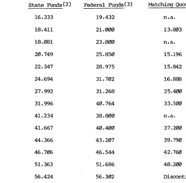
Until 1981 a matching quota was specified by the Commonwealth government for the level of State funds required to be spent on roads as a condition of receiving the grant [4]. Table 2.1 shows the quotas required.

The relaxation of the quota was partially related to the then Commonwealth government's federalism policy which was aimed at encouraging the States to accept more responsibility for both revenue raising and expenditure [5].

[2] S.96 reads "During a period of ten years after the establishment of the Commonwealth and thereafter until the Parliament otherwise

provides, the Parliament may grant financial assistance to any State on such terms and conditions as the Parliament thinks fit".

[3] From 1974/75 to 1979/80 the State spent between $2.5m (1974/75) and $12.5m (1976/77) on National Highways. BTE, "Australian Road Financing Statistics 1970-71 to 1979-80", Information Paper 3 (AGPS 1982).

[4] Quotas applied to each category of road included in the Conmonwealth grants, although local government was not subject to matching provisions. [5] Another possible step in this policy is that specific road grants

TABLE 2.1

State and Commonwealth Road Construction & Maintenance Rinds and Matching Quotas, 1968/69 to 1981/82 ($m)(1)

Year State Funds (2) Federal Funds (3) Matching Quota

1968/9 16.333 19.432 n.a.

1969/70 18.411 21.000 13.803

1970/1 18.081 23.800 n.a.

1971/2 20.749 25.850 15.196

1972/3 22.347 28.975 15.842

1973/4 24.694 31.702 16.888

1974/5 27.992 31.268 25.400

1975/6 31.996 40.764 33.500

1976/7 41.234 38.800 n.a.

1977/8 41.667 40.400 37.200

1978/9 44.366 43.207 39.790

1979/80 46.706 46.544 42.760

1980/1 51.363 51.686 48.200

1981/2(4) 56.424 56.302 Discontinued

n.a. Not available

Notes (1) Source Highways Department Annual Reports.

(2) Road user charges net of road safety, police traffic services and M.V. Troubridge expenditure plus other income (rent, land sales, etc.) See note (4) and page 12.

(3) Net of Commonwealth planning and research funds, 1974/5-1980/1. (4) Method of accounting changed. It has not been possible

to reconcile the 1981/82 figures with the previous accounting method, thus other income of $9.954m is omitted fram the 1981/82

figure for State funds (see Table A.1, Appendix A).

Commonwealth grants for roads in 1981/82 paid under the Commonwealth

Roads Grants Act, 1981 were $56.30m, covering the following road categories: National Highways $27.24m

Arterial Roads 16.66

Local Roads 12.40

State Charges and the Highways Fund

The grants from the Commonwealth are paid into the Highways Fund, the operation of which is specified in the Highways Act, 1926-82, Part III. The other major source of road funds, State charges on vehicle users are also paid into the Highways Fund. There are three main charges: motor vehicle registration fees, driver licence fees and a levy on the sale of petrol and diesel fuel. The first two of these charges are collected by the Motor Registration Division of the Department of Transport under the Motor Vehicles Act, and paid into the Highways • Fund. Motor vehicle registration fees are charged according to a complicated power/

mass formula for different types of vehicles (commercial vehicle rates in general are higher) but in fact represent a simple linear relationship between the

fee and the power/mass ratio [6]. Driver licence fees are a flat charge every three years. Collection costs, which are deducted prior to the revenue being paid to the Highways Fund, were $9. 538m or 19% of the gross registration and licence fees collections in 1981/82.

The fuel levy is collected under the Business Franchise (Petroleum Products) Act, 1979 which provides for the licensing of persons who sell petroleum products. It is collected by the State Taxation Office of the Treasury Department at a cost of $57,000 or 0.2% of revenue collected in 1981/82 [7].

The fuel levy was introduced in 1979 as a replacement to the former Road Maintenance charge which was a "tonne-km" tax on heavy vehicles. At the time it was introduced motor vehicle registration fees were varied in an attempt to ensure that users of light vehicles did not pay more, and users of heavy vehicles did not pay less with the replacement charges. The structure

[6] Director-General of Transport, Adelaide Urban Transport Pricing Study: 2nd Stage Report, prepared by R. Travers Morgan Pty. Ltd. (Adelaide 1980), p.38. The structure of charges will be simplified on 1 April 1984 when motor cars will be charged based on the number of cylinders, and heavy vehicles on the basis of unladen mass.

of charge: did not appear to be completely successful in this aim. The fuel levy is a percentage of the declared pump price of petrol (4.5%) and

diesel(7.1%) fuels. A legislative procedure is involved to vary the declared pump price [8]. The rates of the charge at the end of 1981/82 were 1.49 c/litre for petrol and 2.53 c/litre for diesel.

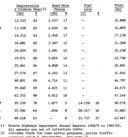
Table 2.2 shads the amounts collected from the various State charges on vehicles and vehicle users over several years. It can be seen that the fuel levy has become an important source of revenue and represented 37%

TABLE 2.2

Composition of Road User Revenues 1968/9 to 1981/2(1)

Year Registration Road Mtce Fuel

%

Total & Licence Fees(2) Charge Levy ($m)

MO % ($m) % ($)-

1968/9 12.533 83 2.557 17 - 15.090

1969/70 13.250 82 2.839 18 - 16.089

1970/1 14.212 83 2.958 17 - 17.170

1971/2 18.001 85 3.287 15 - 21.288

1972/3 18.829 85 3.401 15 - 22.230

1973/4 19.871 84 3.859 16 - 23.730

1974/5 25.841 86 4.050 14 - 29.891

1975/6 27.574 87 4.242 13 - 31.816

1976/7 40.081 89 4.716 11 - 44.797

1977/8 39.848 89 4.825 11 - 44.673

1978/9 42.352 90 4.812 10 - 47.164

1979/80 35.339 70 1.077 2 14.158 28 50.574 1980/81 35.586 64 .050 0 20.167 36 55.803

1981/82 40.210 63 - 0 23.737 37 63.947

Notes (1) Source Highways Department Annual Reports 1968/9 to 1981/82. All amounts are net of collection costs.

(2) Includes funds for road safety purposes, police traffic services and M.V. Troubridge. See page 12.

of all collections in 1981/82. There was a significant fall in collections of motor registration fees (16%) in the year the fuel levy was introduced

(1979) but in total collections increased by 7%.

There are several other miscellaneous revenue items which can be made available for road construction and maintenance. They include rent for properties acquired in advance of road construction, land sales, plant sales, revenue from the

operation of the M.V. Troubridge (see below) and a road maintenance payment from the ST7[9]: these amounted to $10.864m in 1981/82[10]. Table 2.3 shows the composition of all receipts for 1981/82.

Sources of Item

TABLE Road

2.3

Funds (Net) Amount ($m)

Commonwealth grants 56.302

Motor Registration fees $44.435m

Driver licence fees $5.312m ) 40.209

Fuel levy 23.737

Land sales 4.431

Rents 3.224

Plant sales 1.349

M.V. Troubridge revenue 1.810

STA road maintenance .029

Other .021

Total 131.112

Source: Report of the Auditor General, op.cit., p.104

Road Construction & Maintenance

Expenditures by the Highways Department are largely on the construction and maintenance of arterial roads. Some of the Commonwealth local road grant is given direct to local governments ($8.487m in 1981/82) and the remainder plus some State funds ($473,000 in 1981/82) is spent on local roads by the Highways [9] This payment was discontinued on 1 July 1982 by the repeal of S.36a

of the Highways Act, as the STA pays the fuel levy. The charge was previously justified on the grounds that no registration fees were paid for STA vehicles.

on local roads are included in the Highways Department's reported expenditure [11]. Road construction and maintenance expenditure in 1981/82 amounted to $97.113m,

with 65% spent on construction and 35% spent on maintenance.

The amounts expended on the different road categories is Shown in Table 2.4. When National Highways are excluded, the proportion of funds spent on construction falls to 57%.

TABLE 2.4

Road Construction and Maintenance Expenditure by Road Category, 1981/82

Road Category Expenditure ($m)

Construction Maintenance Total

National highways 23.481 4.074 27.555

Developmental .333 - .333

Rural Arterial 10.152 15.970 26.122

Rural Local 4.773 6.895 11.668

Urban Arterial 21.204 6.922 28.126

Urban Local 3.023 .286 3.309

Total 62.966 34.147 97.113

Source: Report of the Auditor General, op.cit., p.107.

[11] Highways Department Annual Report 1981/82. In 1983/84 a new procedure for allocating Commonwealth local road grants will apply: 40% will be retained by the Highways Department and 60% will be allocated on a formula basis to local governments. The formula for distribution between metopolitan and rural councils will be on the basis of equal weighting of road length and population. The distribution between metropolitan councils will be on the same basis while for rural councils the formula will include those two items plus an allowance for "road effort" (reflecting the amount spent fram the council's own resources in the previous year). D. Starkie, "The Specific

Other Expenditures

Under the Highways Act there are certain statutory requirements regarding the uses of the funds collected from motor vehicle charges. Revenue from the sale of personalized number plates, and one-sixth of the revenue fram driver's licence fees are allocated for road safety purposes (Section 32(1)). A proportion of the gross collections of motor registration fees is payable to the Police Department on account of traffic services provided on roads in S.A. by the police (Section 32(m))[12]. The Highways Department is financially responsible for the operation of the M.V. Troubridge which provides passenger and freight service to Kangaroo Island (Sections 31(2) (i) and 32(n)). Expenditure on the service exceeded revenue by $2.1m in 1981/82, and this amount was a charge on the Highways Fund.

Another major payment fram the Highways Fund was $10.843m in the general administration of the Highways Department. Miscellaneous payments amounted to $11.996m in 1981/82 and included such items as planning and research, plant purchases and debt charges. The composition of all expenditure in

1981/82 is given in Table 2.5.

TABLE 2.5

Uses of Road Funds 1981/82(1)

Item Amount ($m)

Construction and maintenance 97.113

Bicycle track construction 0.152

Building and land maintenance and operation 3.303

Planning and Research 1.854

Plant and stores 1.840

General Administration & other expenses 10.843

M.V. Troubridge operation 3.929

Road Traffic Board activities 1.580

Repayment and debt charges on loan funds 1.911

Road Safety(2) 1.049

Police traffic services 4.355

Total 127.929

Notes (1) Source Report of the Auditor General, op.cit., p.104. (2) $1.049m represents receipts from personalised number

plates and allocation for road safety from drivers' licence fees collections. Actual expenditure was $1. 53m from current receipts and accumulated funds. ibid p.105.

- 13 -

Concessions

Concessions on motor registration fees and drivers' licence fees are available to certain groups of people and fees are not charged to other

groups. The revenue foregone fram these concessions and omissions was $10. 163m in 1981/82, made up as follows [13]:

Registrations

- primary producers $ 2.881m

- crown, statutory, local government

and other bodies 2.547

- interstate plates 2.613

- pensioners 1.416

- outer area residents, prospectors .423 Licences

- pensioners .283

$10.163m

In the case of many other concessions a reimbursement is made by the State government on account of concessions, e.g. for public transport, water and local government rates concessions. This is not done for road

funding as it would require a payment from general revenue funds to the

Highways Fund, whereas with the other reimbursement payments it simply requires transfers between budget lines within the state revenue budget. The cost of the concessions could however be relevant in any comparison of revenues and

costs of road use. This would not be the case for all payments above, in particular it is not possible to collect registration fees fran holders

of interstate licence plates as this is considered to be a restraint of trade under S.92 of the Australian Constitution [14]; also where residents of outer areas are not users of public roads a concession may be justified on the grounds of non-use.

[13] Report of the Auditor General, op.cit., p. 179.

Real

TOTAL

Actual

•N,Real

N.CONSTRUCTION - 14 -

Trends in Costs

The amount spent on road construction and maintenance in real terms has fallen in recent years as can be seen from Figure 2.1. The figure is derived from Tables A.3, A.4 and A.5 in Appendix A. The real figures have been inflated to the June 1982 level using the Highways Department road construction cost index. This index rose 19% faster than the CPI fram 1968/69 to 1981/82 (see Table B.1, Appendix 8).

uuu uoi tars

--'-z•MAINTENANCE

--- Actual 180 000 -

170 000 -

160 000 -

150 000-

/40 000 -

130 000 -

/ 120 000

110 000

-

100 000

90 000-

80 000 -

TO 000 -

60 000 -

50 000- Actual

•••• _%

40 000 -, _{■ Real}

,10 IIMIN Min ••■■• Mlint .//Mb. ONO ONO ••■•■ •■•• ..1■• OMB

30000- .

20 000-

„, 10

o

1968/1969/1970/1971/1972/19734974/1975/1976/1977/1978/1979/1986/1981/1982 .

Year

PUBLIC TRANSPORT FUNDING

Public transport services in Adelaide are provided by the State Transport Authority (STA) which was established in 1974 by combining two public bodies (one for bus and tram, and one for rail services). Soon after establishment, the STA, on the direction of the government, acquired most private companies operating metropolitan bus services, thus giving the STA a virtual monopoly of regular route public tranpsort services in the metropolitan area. The STA operates one tram route, four main suburban rail routes (with six branch lines) and over 100 bus routes.

Recurrent Funding

Road funding is almost solely from current charges on motor vehicles and vehicle users, and from Commonwealth Government grants administered

through a statutory fund. In contrast to this, funding of public transport service is through user charges, and the State Government's revenue and

loan accounts. The STA prepares financial statements as a trading enterprise, and any deficit on current operations (including annual capital charges)

is funded through the State revenue account. Payments for items of a capital nature have generally been through the State loan account. The different methods of funding public transport make comparisons with road funding levels difficult.

The profit and loss statement for the STA for 1981/82 is given in Table 2.6: costs exceeded revenue by $62.286m, giving an overall cost recovery of

then invested and interest earned on the investment. In some years the grant has been more than the deficit, in others less, depending on decisions of the government, presumably taking into account its overall financial position. The accumulated cash reserves of the STA may then be used for capital items.

TABLE 2.6

STA Profit and Loss Statement 1981/82 (1)

Item Amount ($m)

Revenue

Traffic 28.011

Sundry 3.830

Interest 5.873

Total 37.714 37.714

Expenditure

Traffic 36.654

Maintenance 24.525

General Expenses 16.081

Fuel, Oil & Power 7.629

Total Operating Expenditure 84.889

Operating Loss 47.175

Capital Charges

Depreciation 5.418

Lease payments 2.171

Interest on Loans 7.522

Total capital Charges 15.111

Total Expenditure Total Loss

100.00

62.286 Comprising:

- Contribution from Revenue Account - Decrease in cash reserves held by STA

55.350 6.936

The first lease payments for the purchase of buses were made in 1981/82. This form of financing is likely to increase in the future so that the potential for the accumulation of cash reserves will decrease along with interest earned on investments; the effect on the STA accounts will be to increase the deficit, although all that has happened is a change in the method of financing rollingstock purchases.

Trends in Costs of Operation

•••••#. •

..•••••■••

100 000

90

000-80 000,

70 000 -

60 000 -

50 000-

40 000 -

30 000 -

20 000 -

10 000

'000

Do

llars

COST

• DEFICIT

••••-•

••••••

REVENUE

■

—..-

ase

0

1968/1969/1970/1971/1972/1973/1974/1975/1976/1977/1978/1979/1980/1991/1982

•

Year

Fig. 2.2

Public Transport Costs ei Revenues

1968/69 to 1981/82

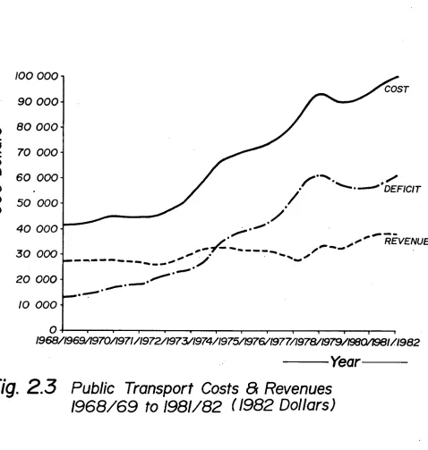
Costs have risen at a much faster rate than the CPI, While revenue has remained relatively constant over the same period. The large increase in costs in the mid-1970s was associated with the acquisition of the privately operated bus services in Adelaide by the STA [15]. The acquisition

resulted in the STA bus fleet almost doubling in size. The increase in public transport costs constrasts with expenditure on roads Which has fallen in real terms (see Figure 2.1).

[15] P.G. Kain, Urban Transport Crisis - A Study of Adelaide Bus Operations in Transition 1967-81, Honours Economics Thesis (unpublished)

100 000

90

000-80 000 -

70 000 -

60 000 -

50 000 -

40 000 -

30 000 -

5.3

COST

DEFICIT

•

_■

---

...•■••••

■•■••■■...am

4.1.10

20 000 - _• ••••••••• •

10 000 -

0 •

1968/1969/1970/1971/1972/1973/1974/1975/1976/1977/1978/1979/1980/1981/1962

Year

Fig. 2.3

Public Transport Costs 8r Revenues

1968/69 to 1981/82 (1982 Dollars)

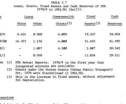
Capital Funds

- 20 -

TABLE 2.7

Loans, Grants, Fixed Assets and Cash Reserves of STA 1978/9 to 1981/82 ($m)(1).

Year Leans Commonwealth Fixed Cash

State Other Grants (2) Assets (3) Reserves

1978/9 6.431 .0.968 4.089 19.327 34.854 1979/80 16.357 1.156 4.000 21.455 41.995

1980/1 - 1.087 4.500 2.807 38.542

1981/2 - 0.958 - 11.034 29.511

Notes (1) STA Annual Reports. 1978/9 is the first year that integrated accounts are available.

(2) Grants under the States Grants (Urban Public Transport) Act, 1978 were discontinued in 1981/82.

(3) This is the increase in fixed assets, without adjustment for depreciation.

Concessions

Included in the Traffic Revenue of the STA are reimbursements on account of the carriage of passengers at concession fares. In 1981/82 these amounted to $5.755m, and are a payment by the State government in addition to the deficit for the operation of public transport in Adelaide. The reimbursement payments comprise:

Pensioners, blind and incapacitated $2.860m

Students 2.030

Unemployed .865

$5.755m

OTHER TRANSPORT FUNDING

The other major source of expenditure on transport by the S. A. government relates to the operation of the Department of Transport and the Department of Marine and Harbours. The main functions of the Department of Transport are the provision of policy and administrative support to the Minister of Transport, planning & research, collection of motor vehicle fees, road

constructs and operates the State-owned ports in S. A., and has responsibility for the safe operation of recreational boating and same aspects of the

fishing industry.

Department of Transport

The Department of Transport is a net cost to the State revenue budget as the bulk of the revenue it collects is paid into the Highways Fund (after deduction of collection costs). Table 2.8 shows the recurrent revenues and costs for the Department of Transport in 1981/82; there was a net cost to the State revenue budget of $2.454m. Other expenditures are made through the Department of Transport budget and in 1981/82 these were:

- $877,000 from the loan account for planning and research projects [16]; - $3,414,000 from the revenue account for concessionary travel by various

groups on various services [17];

- $256,000 from the revenue account for subsidies for the operation of country town bus services [17]; and

- $99,000 from the revenue account for grants for the establishment of community bus services [17].

Department of Marine and Harbours

The Department of Marine and Harbours (DMH) operates six major ports in S.A. and several smaller ports, jetties, etc. The accounts for the EVE are

prepared partially along commercial lines. Interest is charged on loan funds used for capital purposes, however there is no charge for the depreciation of capital assets operated by the DMH. In 1981/82 revenue of the Department exceeded operating costs by $8.157m however when capital charges (no depreciation) were included a deficit on operations of $3.649m resulted. This amount is the net cost to the state revenue budget.

Loans for capital projects amounted to $5.916m, increasing the total loans to the DMH to $108.261m as at 30th June, 1982. Table 2.9 shows the main revenues and costs for the operation of ports where some state responsibility occurs.

TABLE 2.8

Department of Transport Revenue Funds, 1981/82(5) ($ 1 000) (i) Departmental Operations

9,538 832 Revenue

Motor vehicle fees 49,747 less Highways Fund 40,209 Cammissions(1)

Road Safety & Motor Transport - Highways Fund(2) 1,049 - Commonwealth grant 19

- Other(3) 214

1,282 Government Motor Garage 217

Other 12

11,881 Expenditure

Motor Vehicles 8,094

Road Safety 1,603

Government Motor Garage 1,380 Administration 442 Planning & Research 669 Departmental overhead(4) 2,147

14,335 Net cost to State revenue budget 2,454 (ii) Other Recurrent Expenditures

Transport Concessions (6)

Pensioners 3,078

Australian National 156

Incapacitated 145

Blind 35

3,414

Country Town Bus Services 256

Community Bus grants 99

3,769

NuLes (1) MRD collects fees on behalf of other Deptartments, for which it receives payment.

(2) Actual payment to Road Safety Fund. Expenditure was $1.530m including drawings from previous years collections.

(3) Mainly Licence fees for passenger bus licensing, vehicle inspection fees.

(4) Includes building maintenance, superannuation. Also covers Division of Recreation & Sport which was a Division of Department of Transport from 1979 to 1983.

(5) Source Report of the Auditor General, op.cit., p.176-7.

TABLE 2.9

Department of Marine & Harbours Revenue Funds, 1981/82( 1) ($'000)

Revenue

Wharfage & Tannage 14,793

Pilot Fees 4,207

Bulk Handling Charges 4,759

Fishing Industry 187

Conservancy Dues 1,149

Total 25,095

Expenditure

Management 6,367

Operating & Maintenance 10,047

Fishing Industry 524

Total 16,938

Operating Profit 8,157

Debt charges(2) 11,806

Net cost to state revenue budget 3,649 Notes (1) Report of the Auditor General, op.cit., p.124

(2) Includes interest, Sinking Fund Contributions and Superannuation.

USER CHARGES

Many user charges have been discussed above, however other fees do exist which have not been considered as they are not used for transport funding. Some of the charges may be regarded as general taxes, but all are included here for campleteness.

State charges on road users are:

- motor vehicle registration fees which vary from $8 p.a. to $3929 p.a. depending on the power mass of the vehicle and whether it is used for cammercial or non-commercial purposes. Total collections were

$44.435m in 1981/82

- stamp duty on new registrations and transfer of registrations. Total collections were $21.760m in 1981/82, this amount being credited to the State revenue account [18]

- compulsory third party (CTP) insurance which is solely offered by the State Government Insurance Commission (SGIC). The amount of the charge varies with the class of vehicle (based on accident analysis), and $90.717m in premiums was collected in 1981/82 [19]

- stamp duty on CTP insurance which amounted to $2.013m in 1981/82, is paid into the Hospitals Fund as a contribution to the difference in hospital charges and costs on account of road accident patients [18] - _{State fuel levy of 1.49 c/litre on petrol and 2.53 c/litre on diesel.} Collections amounted to $23.737m in 1981/82 of which approximately 77% is attributable to petrol. The Commonwealth government also imposes charges on fuel through excise duty and the import-parity levy.

The exise in 1981/82 was 6.155/litre (including 1 cent/litre for the ABRD programme) for both petrol and diesel. The collections amounted to

$970m throughout Australia in 1981/82.

The only charges on STA public transport users are fares which vary between zero and 90c per journey depending on the class of user, the length of

journey, and the time of journey. Revenue from fares (including reimbursements for concession riders) amounted to $28.011m in 1981/82.

Various charges on users of port facilities are made (see Table 2.9). Collections amounted to $25.095m in 1981/82.

Table 2.10 summarises the amounts collected from transport users as state charges in 1981/82.

[18] ibid, p. 177.

TABLE 2.10

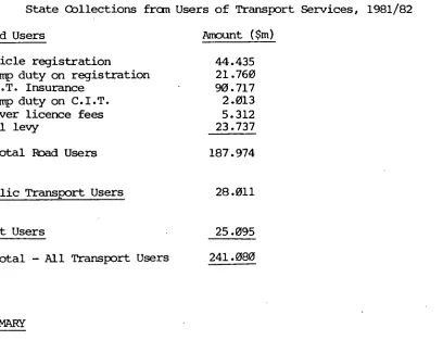
State Collections from Users of Transport Services, 1981/82

Road Users Amount ($m)

Vehicle registration 44.435 Stamp duty on registration 21.760

C.I.T. Insurance 90.717

Stamp duty on C.I.T. 2.013

Driver licence fees 5.312

Fuel levy 23.737

Total Road Users 187.974

Public Transport Users 28.011

Port Users 25.095

Total - All Transport Users 241.080

SUMMARY

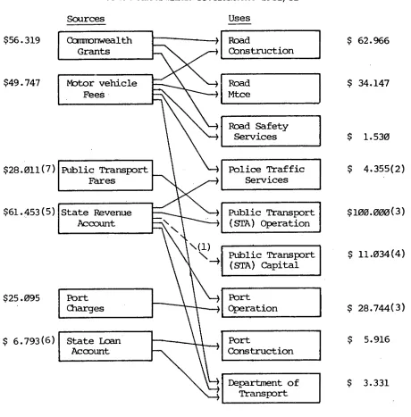
Figure 2.3 summarises the major flows of funds for transport purposes in S.A. in 1981/82 which involve the State government. The major source is the

State revenue account, followed by Commonwealth grants for roads and motor vehicle fees. Despite the differences in accounting, the public transport system still appears to require a larger proportion of state revenue funds (as a consequence of low user fees) than either roads or

ports. Public transport fares represent only a relatively small proportion of the cost of operating public transport services (33% of operating

costs and 28% of total costs), in contrast to ports and roads.

The major use of funds is for the operation of public transport. It

should however be noted that this amount includes annual capital charges, both depreciation and interest, or lease payments. NO depreciation is included in the DMH accounts, While no capital charges on the road. stock are

The description of transport costs and revenues presented is restricted to effects on the State budget for transport purposes. A complete picture of transport expenditures would include other direct costs to the government and externalities associated with transport. Direct costs could include costs to the public hospital system as a result of road accidents and which are not recovered fram hospital users [20]; and police traffic services (the payment from the Highways Fund does not cover the cost of these services [21]). Externalities could include accidents (the loss to society through lost production) and various forms of pollution generated by transport activities.

[20] Director-General of Transport, Adelaide Urban Transport Pricing Study: Interim Report, prepared by R. Ttavers Morgan Pty. Ltd. (Adelaide 190), para B.15.

Sources

I

$56.319 Commonwealth Grants 111140 mdaL Fees Uses Road Construction Road Mtce $49.747 Motor vehicle

Public Transport Fares Port Charges Road Safety Services Police Traffic Services Public Transport (STA) Operation Public Transport (STA) Capital Port Operation Port Construction Department of Transport $28.011(7) $25.095

$61.453(5) State Revenue Account

(

$ 6.793, 6 ) State Loan Account

FIGURE 2.3

Major Sources and Uses of Funds for Transport South Australian Governmnent 1981/82

$ 62.966

$ 34.147

$ 1.530

$ 4.355(2)

$100.000(3)

$ 11.034(4)

$ 28.744(3)

$ 5.916

$ 3.331

Notes (1) This is an indirect flow as a consequence of the method of funding the STA deficit. See page 15.

(2) Only the share of cost paid through the Highways Fund. (3) Includes annual capital charges (depreciation, interest and

lease payments.

(4) Capital expenditure from internal sources, see page 19. (5) $55.350m for STA deficit, $3.649m for DMH deficit

and $2.454m for DOT. Excludes Police services - see Note (2). (6) $0.877m for DoT and $5.916m for DMH.

CHAPTER 3 INVESTMENT AND PRICING THEORY

INTRODUCTION

As stated in the introductory chapter the aim of this thesis is to determine optimal investment levels for urban transport services provided by the

government of South Australia. The concentration is on the provision of arterial roads and public transport services in Adelaide. These represent approximately 50% of the total State expenditure on transport services throughout South Australia.

The urban optimization procedure is based on existing published work on optimal congestion tolls for urban freeways in the United States, and on optimal subsidy levels for public transport in the United Kingdam. This chapter describes that work and other work relevant to the problem under study. The theory described determines optimal price levels, from which will flaw optimal investment levels. The road approach is "first-test" but it is arguable whether the optimal tolls can be collected in practice because of institutional and political constraints. The option of second- best pricing of the competing public transport modes is therefore considered in order to achieve the optimal flaw level on the (optimal) road capacity.

MARGINAL COST

AVERAGE COST

DEMAND

Traffic Volume

OPTIMAL ROAD TOLLS

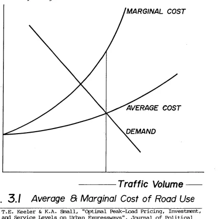
Keeler and Small [1] have developed a model for optimal charges for urban free-ways in the Bay Area of San Francisco. The model is formulated to maximize the net benefits (benefits minus costs) of the freeways. Benefits are measured in terms of demand (vehicle miles of travel), and costs in terms of road construction (including land acquisition) and maintenance costs, and private road user costs, i.e. travel time. Travel time provides the marginal social cost component of the model, i.e. an extra vehicle imposes extra cost on all other vehicles currently using the road so that the marginal cost is above the average cost of road use. This marginal social cost increases rapidly at higher traffic volumes. The effect is presented diagramatically in Figure 3.1.

Fig. 3.1

Average

&

Marginal Cost of Road Use

Two basic assumptions of the model are that road plant is divisible and that demand in each period is independent. With respect to the former assumption Keeler and Small contend that this:

ft _{is not an unreasonable assumption for large urban} highways, for the wider the roads in the system, the less relevant indivisibilities become to the analysis" [2]

In their estimation however a lane is used as the extra unit of capacity; this simplification tends to weaken the assumption of divisibility of plant. The alternative of estimating the model with small increases in capacity, such as improved dhannelization at intersections and/or the implementation of parking bans at heavy traffic flaw times (Clearways) [3], would introduce complexities into the road cost estimation and may make the n el inoperable. Estimating the model with the implicit assumption that an extra lane is the only means to increase output (capacity) appears to be a weakness [4].

Keeler and Small treat their second assumption, i.e. independent demands, by undertaking sensitivity testing of the results. These tests are

carried out by making assumptions About the likely spreading to other time periods that would occur if optimal tolls were introduced. The model is based on peak load pricing theory [5].

[2] ibid, p.2.

[3] In this case the extra capacity is gained through improved management of plant, not an increase in plant as such.

[4] D.N.M. Starkie, "Road Indivisibilities", Journal of Transport Economics & Policy (September 1982). Here it is argued that indivisibilities are small, particularly for rural Australian roads, as capacity may be increased by many measures other than extra lanes, e.g. width of the lane, its curve and/or gradient.

Specifically, the Keeler & Small model maximises the net benefits (NB) of all trips over the life of the road:

T ErQt

NB =

₅

where T is the life of the road. is the time period.

Qt is the flow of vehicle trips over a given route per unit time. Pt is the total user cost of a trip (including travel time).

Ct is the average variable cost (user and publicly supplied inputs) that vary with vehicle miles of travel.

is the size or width of the road.

p(w) is the cost of road provision which varies with width of the road. The road cost function, p(w), comprises 3 elements: annual rental for the investment in the road, both construction rental and land acquisition rental, and road maintenance costs. Formally the function is:

p(w) = l_e-rL K(w) + M(w) + rA(w)

where r is the interest rate. ,

is the effective life of the road.

K(w) is the construction cost as a function of width. M(w) is the maintenance cost that varies with width. A(w) is the land acquisition cost as a function of width.

In their estimation of road costs Keeler and Small use the number of lanes which comprise a road, as a proxy for width or road size.

The two relevant conditions for maximizing net benefits occur when NB is differentiated, firstly with respect to each Qt:

Pt = Ct + Qt

d Cf

and secondly with respect to w:

-:>: Qt dCt - p s (w) =0 (1)

t=1 dw

This states that the number of lanes should be expanded to the point where the marginal cost of an extra lane is equal to the marginal value of

user cost savings brought about by that investment.

To use the model, the function p(w), and a speed flow curve for the urban freeway system are estimated. The speed flow curve takes the form:

V/C = a + bS - cs2

where V is the volume of traffic per hour

C is the capacity (based on engineering standards) V/C is the volume capacity ratio

a, b & c are estimated parameters S is the speed in miles per hour

The time taken for each trip, which determines the congestion toll portion of the cost of a trip is simply 1/S. To convert time to a monetary-value, a value of time and data on vehicle occupancy are required. Based on accepted engineering standards Keeler & Small use a lane capacity (C) of

2000 vehicles per hour.

Keeler and Small optimize the prices in each period and the overall investment level in a two step process:

(i) An optimal investment policy is determined such that for any given traffic level, total costs are minimized according to (1) above. The actual output is an optimal volume capacity ratio as a function of lane capacity costs (construction, land acquisition and maintenance), and tine values (from the speed flaw relationship).

(ii) Given the optimal volume capacity ratios, the optimal long run price for each period is determined. Of interest is the congestion toll component of the price.

congestion tolls). This is not the case with the Keeler and Small model where prices and capacity are both operated on to improve the level of service (volume capacity ratio).

The results of the application of the model to the Bay Area suggest that in the mid-1970s when their research was undertaken the optimal price levels were well in excess of existing user charges. Fr example in the peak periods on downtown freeways, tolls between 14.5 and 31 cents/vehicle mile are estimated compared to the user charges at the time of 1.15 cents/ vehicle

mile. On the other hand at the lowest demand times, a toll of 0.2 cents/vehicle mile is the optimal level.

The practical problems of collecting tolls on urban freeways are given only scant attention by Keeler and Small [6]. The problems would be greatly magnified on urban arterial roads (because of the greater difficulties of controlling entry and exit) unless perhaps they are collected by means of a tax on fuel. This method raises issues to be addressed when formulating the policy to be adopted in setting road user charges. In particular, are there greater or smaller efficiency losses by charging the high demand (peak) toll at all times relative to charging the law demand (off peak) toll at all times; and is there a further second-best option that is feasible, e.g.

subsidizing public transport to achieve a switch from road use to public transport use during periods of high demand thus enabling the optimal road volume capacities to be achieved even though the optimal (peak) toll cannot be charged.

Varying Tolls with Demand

Walters [7] refers to the problem of the level of congestion tolls with respect to urban (congested) and rural (uncongested) roads where

they are collected by means of tax on fuel. He is mainly concerned with

[6] Keeler & Small, op.cit., p.23.

the problem of urban residents making trips to the country to buy fuel and thus avoid the toll:

"I should have thought that it would be possible to hold this differential in the large urban areas such as New York, Philadelphia, Chicago, and Los Angeles. For the vast majority of the population in these areas, the distance from any rural area, where the elasticity is very low, is usually great enough to prevent gasoline "poaching". For the smaller urban areas surrounded by rural highways with low elasticities the tax differential would probably have to be lower. On the other hand, the motorist who undertakes a long cross-country journey will, of course, be Able to buy gasoline at the km rate of tax. This is desirable since most of his mileage will be on (uncongested) tollways or on freeways between urban areas." [8]

The urban/ rural question is not central to this thesis, however the implications for rural road use of optimal tolls set for congested metropolitan road conditions and charged by means of State-wide fuel tax are mentioned in Chapter 5.

Sherman [9] explicitly treats the question of price levels at different times of the day for two competing modes, car and bus, where it is not possible to vary the charge by time of day (cc level of demand) for the car mode. Sherman's model also includes allowance for the congestion effect of one mode on another, called congestion interdependence. For example an extra car trip will cause increased congestion on the road system thus affecting both car and bus modes.

Sherman concludes:

"...the choice of policies, between rush-hour or off-peak first-best optimality, will depend on the amount of travel and the

seriousness of misallocations in the separate periods. The choice is not an easy or direct one, and a mixture of the two solutions might even be better than either one alone, especially if the amount of travel is nearly the same at the peak as it is at all off-peak times combined". [10]

This issue is not addressed in this thesis but it is possible that the models used could be expanded to do so.

L8J ibid, p.28.

[9] R. Sherman, "Congestion Interdependence and Urban Transit Fares", Econametrica 39, 3 (May 1971), pp. 565-576.

OPTIMAL PUBLIC TRANSPORT FARES

Sherman provides a methodology for determining optimal public transport fares in a second-best environment; another approach is that of Glaister and Lewis [11] which is described below. Jackson [12] has an approach similar to Sherman but does not include congestion interdependence. His diagramatic presentation of the problem is good; it is adopted here to enable explanation of the second-best nature of the problem.

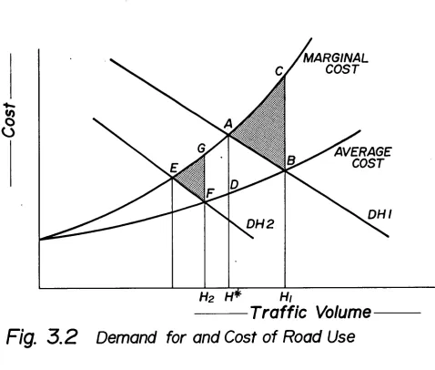
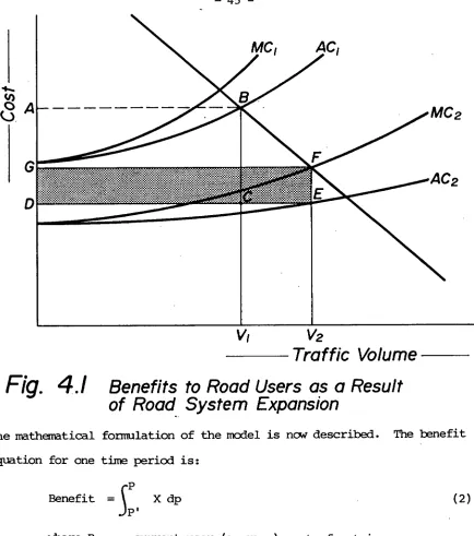
Figure 3.2 shows the demand and cost curves for road use, H1 is the resulting volume of traffic (intersection of demand and average cost curves), While H* is the optimal volume (intersection of demand and marginal cost

curves). The social loss is the triangle ABC, and a congestion toll of amount AD would reduce the volume of traffic to the optimal level, H* and eliminate the social loss. If it is not possible to charge the toll, AD, then a second-best solution is to lower the price on a competing mode so that the volume of car traffic is reduced. This is the short run solution as there is no opportunity to vary capacity. Figure 3.3 shams the demand and cost curves for competing public transport services. There are Tl public transport trips at a fare equal to average cost of ACI. The second-best policy reduces the fare to AC2 by the provision of a subsidy to the public transport operator and this subsidy results in a social loss of ACD in Figure 3.3 and an increase in public transport passengers to T2. The social loss (ACD) is the cost of the subsidy (ABCD) minus the fare revenue fram the increased passengers (ABC).

The second-best policy has increased the social loss: originally the loss on the road system was ABC in Figure 3.2, and now we have created a

[11] S. Glaister & D. Lewis, "An Integrated Fares Policy for Transport in London", Journal of Public Econamics 9 (1978), PP- _341-355-

MARGINAL

COST

AVERAGE

COST

H2

H*

Traffic Volume

Fig. 3.2

Demand for and Cost of Road Use

loss ACD in Figure 3.3. However as a result of the increased public transport usage there will be a decrease in the demand for road travel, shown as DH2 in Figure 3.2. This lower demand causes a smaller social loss

(EFG) on the road system. The net gain (or loss) in welfare as a result of the second-best policies depends on the relative sizes of the three social loss triangles. The net gain is calculated as:

(i) the social loss on the road system prior to the second best policy (ABC in Figure 3.2) minus

(ii) the social loss on the public transport system as a result of the second-best policy (AC) in Figure 3.3) minus

- 37 -

A

o

_AC,

C AC2

7, T

2

Public Transport Trips

Fig. 3.3

.Demand for and Cost of Public

Transport Use

The subsidy to public transport should be designed so that the net welfare gain is maximized. Jackson goes on to make an estimate of the gain based on the demand and cost characteristics of the road and public transport systems. The resulting equations are complicated and are not reproduced here as it is not intended to use the Jackson methodology mainly because it requires estimates of several cost elasticities (as does Sherman) which are not available. The Jackson approach is implicitly only concerned with the peak period, i.e. an assumption is made that there will be no

"Such subsidies may improve allocative efficiency, though no significant improvement is apparent unless marginal social cost per car passenger mile is at least 80 per cent above private cost in the highway sector" [13].

Jackson also notes that the cross elasticity of demand for road travel with respect to the price of public transport travel should be greater than 0.2 [14].

The approach used by Glaister and Lewis for determining a second-best policy for public transport is the one adopted in this thesis. The

model developed by Glaister and Lewis is intended to determine the optimal level of subsidy, given that it is not possible to charge the marginal social cost of road use. Their aim is the same as that of Jackson, but the methodology is quite different. The model is formulated in terms of expenditure functions (G) for both the current and optimal position, and the public transport subsidies (aggregated across all individuals); the expression is maximized and optimal prices and subsidy levels determined. The model allows for 3 modes (car, bus, rail) and 2 time periods (peak, off-peak) giving six types of transport as follows:

1. peak car 2. off-peak car 3. peak bus 4. off-peak bus 5. peak rail 6. off-peak rail.

Formally the model determines optimal prices (p3, p4, p5, p6) by maximizing: {(G (a31 a4 ,a5 ,a6 ,X1 (a3 •••,a6 ),X3 (a3 •••,a6),p,u)

-G (p3 ,p4,p5 ,p6 ,x1(p3 •••,p6 ),x3(p3 •••,p6 ),p,u)

4c3(xl,x3) - 10,3x3] - [C4 (X4) - R4x4]

-[C5 (X 5 ) - p5X5 ] - [C6 (X6) - p6X6] / where G is the expenditure function

p3,104,135,p6, are the variable public transport prices

p is the vector of all other (fixed) prices including pi and p2 u is a vector of constant utility levels

a3. ..,a6 are a set of base prices for modes 3...,6 C3...,C6 are the costs of operating modes 3...,6

The difference between the expenditure function evaluated at the base (a) prices and the optimal (p) prices is the compensating variation, i.e. the change in expenditure required to maintain a constant level of utility as prices increase from p3 ,..p6 to a3 ,..a6 . The volumes of peak car travel (X1) and peak bus travel (X3) are included in the top two lines of the expenditure function because of the congestion effects of these two modes, i.e. in

Sherman's terminology the model allows for congestion interdependence .

When the expenditure function is differentiated with respect to p3,..p6, and converted to elasticity form, a linear system of equations is obtained:

(p3-S 3 )X3 e 1

(p4-C1)X4 S iXi e4 (p5-Cg)X5

(136-e)X6 4

where e are income compensated elasticities, and el is the elasticity of demand for mode 3 with respect to the price of mode 4.

S1 and S3 are the marginal social costs of peak car and bus traffic respectively where:

S1 = dG + dC3 and S3 = dG + dC3

dX1 dX1 dX3 dX3

-e3 ei e§ eS- ei el e/ e/

Glaister & Lewis interpret the system of equations as follows:

"...both peak and off-peak prices will be below respective marginal social costs by an amount proportional to marginal social costs of car, use, both because of the possibilities of attracting peak car users directly (througll el and 4) and reallocating demand between periods (through el and ei) so as to allow further adjustment to car traffic"[15].

Glaister and Lewis proceed to use the model to estimate optimal fare and subsidy levels for London's public transport. The use of income compensated elasticities makes little difference to the results as the share of

expenditure spent on the public transport modes is low (0.0027 to 0.0076)[16].

The marginal social cost of a peak bus was assumed to be 0.05 pence per passenger mile. It was more difficult to obtain data on the marginal social costs of peak car travel so two cases were tested, both arbitrary. Use of a speed flaw relationship for London could have provided the means of estimating the marginal social cost of car travel.

The Glaister and Lewis model is formulated in terms of price, while service quality is another, often more important, determinant of demand for transport services[17]. The marginal costs of the public transport modes used are private, i.e. costs to the operator, while the marginal

social cost of car travel is used. When considering public transport pricing Turvey & Mdhring claim:

"The right approach is to escape the notion that only costs which are relevant to optimization are those of the bus operator. The time-costs of the passengers must also be included too, and fares must be equated with marginal social costs" [18].

[15] Glaister & Lewis, op.cit., p.346. [16] ibid, Table 2, p.349.

[17] S. Glaister, Fundamentals of Transport Economics, Basil Blackwell (Oxford 1981).

A positive externality is associated with the use of scheduled public trans-port services, often termed the frequency benefit, which leads to decreasing marginal social costs [19]. More services mean decreased waiting times to existing passengers, or decreasing social costs as output increases. This omission appears to be a weakness in the formulation of the model. It is however not clear haw the omission would effect the Glaister and Lewis model. As Waters [20] notes regarding scheduled public transport services:

"There are several other sources of delay and inconvenience costs borne by users whidh also involve externalities, some of them are negative such as congestion delays and crowding. The latter tend to be important on heavily travelled routes, i.e. those where the

increasing returns just discussed are not so important. There are also possible increasing returns to producers, i.e. the traditional sources of decreasing costs. Thus, several factors are involved in determining optimal prices for scheduled transport services and it is not necessarily the case that the increasing returns will dominate. Optimal pricing could result in either a financial deficit or surplus".

For their preferred application in London, the Glaister and Lewis model produced all prices below cost (as expected), peak bus fares just over twice those of the off-peak, peak rail fares thirteen times those of the off-peak, and subsidy and car traffic levels approximately in accord with what existed at the time in London. The results are interesting in light of Jackson's conclusion that the cross elasticity of demand for car travel with respect to bus price should be greater than 0.2 for subsidies to be effective. Glaister and Lewis use cross elasticities of 0.025 (bus) and 0.056 (rail) [21] and suggest significant subsidies. This may indicate that their model formulation is sensitive to the elasticity values used, or alternatively could result from a high differential between social and private car costs in London. As noted above Jackson suggests the differential must be at least 80% for second-best pricing of public transport to be a viable option.

[19] J.O. Jansson, "Marginal Cost Pricing of Scheduled Transport Services",

Journal of Transport Economics and Policy (Septemher 1979), pp. 268-294. [20] W.G. Waters II, "Recent Developments in the Economics of Transport

Regulation". Canadian Transport Commission, Research Seminar Series,

8 Spring 1982), p. 19.

OTHER SECOND-BEST APPROACHES

Train [22] has used the Boiteux [23] solution to the second-best pricing

of BART (rail) and A.C. Transit (bus) in San Francisco. The solution of

problems of this general type, however require the imposition of a budget

constraint, for example a breakeven position if marginal costs are less

than average costs. For the Train case the budget constraint used is

that BART cover its operating costs and that A. C. Transit cover its

total costs. The prices are then optimized within the total budget

constraint for the two nodes.

The use of this approach for determining the price of and investment in

urban arterials in Adelaide does not appear appropriate for two reasons.

Firstly, as mentioned previously the thesis is aimed at determining

appropriate funding levels whereas funding is a constraint in the Boiteux

method. Secondly, it is more difficult to apply the method to the publicly

funded road system where congestion occurs. An analysis comparable to

this has recently been applied by Taplin & Waters [24] to the carriage of

interstate freight in Australia. The two nodes considered are road and

rail, and the budget constraint the existing "public revenue surplus",

over marginal costs. For road freight the budget constraint applies to

the road system rather than the freight services, and optimal prices are

enforced by charges on the use of roads.

[22] K. Train, "Optimal Transit Prices under Increasing Returns to Scale and a Loss Constraint", Journal of Transport Economics and Policy 11, 2 (May 1977), pp. 185-194.

[23] M. Boiteux, "On the Management of Public Monopolies Subject to Budgetary Constraints", Journal of Economic Theory 3 (1971).