Sensitivity analysis of traffic congestion costs in a network under a charging policy

(1)

This is a repository copy of Sensitivity analysis of traffic congestion costs in a network under a charging policy.

White Rose Research Online URL for this paper: http://eprints.whiterose.ac.uk/87450/

Version: Accepted Version

Article:

Mussone, L, Grant-Muller, SM and Laird, J (2015) Sensitivity analysis of traffic congestion costs in a network under a charging policy. Case Studies on Transport Policy, 3 (1). pp. 44-54. ISSN 2213-624X

https://doi.org/10.1016/j.cstp.2014.03.001

© 2014, World Conference on Transport Research Society. Published by Elsevier Ltd. Licensed under the Creative Commons Attribution-NonCommercial-NoDerivatives 4.0 International http://creativecommons.org/licenses/by-nc-nd/4.0/

[email protected] https://eprints.whiterose.ac.uk/ Reuse

Unless indicated otherwise, fulltext items are protected by copyright with all rights reserved. The copyright exception in section 29 of the Copyright, Designs and Patents Act 1988 allows the making of a single copy solely for the purpose of non-commercial research or private study within the limits of fair dealing. The publisher or other rights-holder may allow further reproduction and re-use of this version - refer to the White Rose Research Online record for this item. Where records identify the publisher as the copyright holder, users can verify any specific terms of use on the publisher’s website.

Takedown

If you consider content in White Rose Research Online to be in breach of UK law, please notify us by

(2)

SENSITIVITY ANALYSIS OF TRAFFIC CONGESTION COSTS IN A

NETWORK UNDER A CHARGING POLICY

Lorenzo Mussone, Politecnico di Milano, ABC, Via Bonardi 9, Milano, 20133, Italy,

[email protected] , +39 02 23995182 (corresponding author)

Susan Grant-Muller, Institute for Transport Studies, 36-40 University Road, University of Leeds, Leeds LS2 9JT, United Kingdom, [email protected]

James Laird, Institute for Transport Studies, 36-40 University Road, University of Leeds Leeds LS2 9JT, United Kingdom, [email protected]

ABSTRACT

The costs of congestion can be measured using three approaches: the total costs, the marginal

costs and the ‘excess burden’. Understanding variation in these measures with particular policies is important for planning and resource management. Assessing the cost distribution (e.g. according to priority routes or urban segments) is key to assessing the delivery of both transport objectives and wider social objectives. The aim of this research is to illustrate how the costs of congestion vary with policy-related demand changes around the city of Milan. The case study used is the “Cerchia dei Bastioni” (called for administrative purposes Area C). This is an old urban area within the inner centre of City of Milan network, with a ‘real life’ charging policy that is applied to private vehicles. A large number of scenarios with differing demand levels and elasticities by vehicle classes were explored and equilibrium assignment used to assign demand to the network. Alternative measures for congestion costs were calculated along with other link parameters. Further data collection, including a parallel field survey of changes in PT speed, was also undertaken.

The results indicate a high degree of correlation between changes in the different measures of congestion and changes in vehicle speed (at different levels of demand). Changes in the total cost of congestion are, however, more marked than changes in the Excess Burden of

Congestion. Sub-optimal conditions appear to exist in certain parts of the network which (it is conjectured) arise as a consequence of the configuration of the network i.e. the presence of one way streets and vehicle restrictions. Identifying a more optimal network is left for further research, as is identifying the precise conditions for which vehicle speeds can be used as a proxy for changes in congestion.

(3)

1. INTRODUCTION

Congestion is seen as an issue in urban networks as well as inter-urban environments and as such it features heavily in regional, national and supra-national transport policies.The European Commission white paper (2011) proposed that congestion in the European Union (EU) is often located in and around urban areas and costs nearly 100 billion Euro (or 1% of the EU's GDP) annually. Congestion is invariably regarded negatively and it is seen as a limiting factor on economic efficiency as well as a source of pollution. One common policy approach associated with the costs of congestion is that of road charging schemes (for example in Stockholm (City of Stockholm, 2005)), where an understanding of the costs of congestion may create a more conducive public-acceptance of the scheme and also set an economic framework within which charges may be set.

This research is concerned with an investigation around the sensitivity of traffic congestion costs in Milan. In particular, how these costs vary with a charging policy specifically introduced to reduce congestion but with a secondary goal to achieve environmental

improvements. The starting point is to consider the definition of congestion and how the costs of congestion may be measured. The calculation of congestion costs requires the use of a transport model and as such it is resource intensive for city authorities to monitor. The paper then continues to consider whether vehicle speeds can act as a proxy for congestion costs for the purposes of monitoring. A specific evaluation concerning speed changes for public transport after the charge is presented.

The principal contribution of this paper therefore is to illustrate how the different costs of congestion vary with policy-related demand changes around the city of Milan and how they also relate to vehicle speeds. The findings have particular relevance and implications for city policy makers by illustrating the methodology used to measure the different congestion costs in a practical and real environment, given what tools may be readily available to them. Due to the complexities of measuring the costs of congestion, the examination of the changes in vehicle speeds as a proxy for congestion costs has a strong policy interest – particularly where congestion reduction targets have been set. The analysis presented here has also highlighted specific outcomes that would be of interest to policy makers wishing to build a case for charging schemes in particular contexts, for example, changes in bus speeds following the introduction of charges. Whilst based on a firm existing theoretical foundation, the essence of the paper is as a case study rather than a theoretical exposition. The aggregate picture is made up of a number of disaggregate calculations, a sample of which are presented here. Our goal in the paper is to present information at a level that might be of interested to policy makers and as such is likely to be of interest to a broad range of transport sector stakeholders.

(4)

2. CONGESTION AND ITS COSTS

Despite frequent use of the term, the concept of congestion is often understood but less frequently defined. Congestion can be present as a physically measureable phenomena but perceived congestion (by users of the road network, residents and others) may be as important as the more objective evidence in driving the need for policy measures. The definition given by the Highways Agency (1997) captures the wide understanding of congestion as: ‘the

situation when the hourly traffic demand exceeds the maximum sustainable hourly throughput

of the link.’ Alternatively, Goodwin (2004) defines congestion as ‘the impedance vehicles impose on each other, due to the speed-flow relationship, in conditions where the use of a

transport system approaches its capacity’. In addition, the evidence to date is that congestion, however defined, is closely linked to externalities that include environmental impacts (Barth and Boriboonsomsin, 2008) and safety (Brownfield et al, 2003). In the case of the first, the

presence of congestion leads to a driving behaviour that includes frequent ‘stop-start’ and periods where the engine is near stationary with the engine idling, leading to increases in emissions of local pollutants. In the case of safety, congestion can lead driving behaviour whereby vehicles have reduced headways, drivers may lose attention to the driving task or (due to frustration) take risks in the task, increasing the accident rate. It is clear on an intuitive basis that congestion results in a set of costs – to the driver, other traffic network users, residents and the environment. On a more rigorous basis, it is possible to not only define congestion but to calculate the costs of congestion and link these calculations to future policy priorities and instruments. Grant-Muller and Laird (2007) give an elaboration of two

fundamental approaches to interpreting congestion: firstly a ‘traffic engineering’ perspective (which underlies many measures of congestion) and secondly an economic view (related to principles behind marginal costs of congestion). At the practical level of measuring

congestion, approaches fall into four approximate classes comprising travel time (or speed) based measures, volume based measures, area based measures and summary indices (or more complex model outputs). This also opens other questions about reliability and the costs of traffic estimation (Waadt et al., 2009). More recent definitions have taken a three-dimensional

concept of congestion, for example Marfia and Roccetti (2011) who define a road to be ‘in a

congested state (be it high or low) when the likelihood of finding it in the same congested state is high in the near future’. Moran and Koutspooulos (2010) frame a definition of congestion from the users’ perspective and as a stochastic process. In practice, the simpler measures are more commonly applied than relatively complex measures. Bilbao-Ubillos (2008) indentifies eight main costs (most of them financial and environmental), to measure the total cost of congestion in comparison to smooth traffic flows.

All networks, whether they are telecommunication networks, energy networks, transport, etc. are subject to congestion (Shy, 2001; Mayer and Sinai, 2003). Congestion arises in networks due to a mixture of network properties including the sunk costs of construction, invariant capacity and the fact that networks invariably operate under conditions of economies of scale, scope or density. From a policy perspective it is therefore essential that any network,

(5)

the ability of the owners/managers to expand that network. The price to access and use the network needs to be efficiently managed so as to ensure excessive prices are not charged, and that operating, renewal/investment costs are recovered to an appropriate degree. In a transport context, policy commentators often estimate the costs of congestion as part of this debate – particularly the aspect of the debate related to the provision of additional capacity. This has led to a wide range in the estimates. For the UK, for example, the range extends from £2 billion per year (Dodgson et al., 2002) to the often quoted Confederation of British Industry (CBI) estimate of £20 billion per year (CBI, not dated, cited in Grant-Muller and Laird, 2007). In this case there exists a factor of almost 10 between the estimates.

This large range stems from the fact that there are two principal definitions for the cost of congestion: the total cost of congestion (TTC) and the excess burden of congestion (EBC) (Grant-Muller and Laird, 2007). The Total Cost of Congestion effectively compares the current or predicted situation against a reference state of zero congestion. The concept is illustrated in Figure 1 where the Total Cost of Congestion is given by area A. In this figure V0 trips experience a journey time cost of UC0, whereas in the absence of congestion the cost experienced would be UCno congestion. In contrast the Excess Burden of Congestion is the deadweight loss that congestion imposes on society. This is illustrated in Figure 2 by Area B. The deadweight loss arises as users of transport networks invariably do not face the full marginal social costs (MSC) of travel. Marginal external costs of congestion (MECC)1 (and therefore demand for travel) exceed optimum levels. Congestion levels also exceed optimum levels. This is illustrated in Figure 2, where the marginal private costs (MPC) are illustrated as well as the marginal social costs (MSC). The difference between the two is the marginal external cost of congestion (Walters, 1961, Glaister, 1981; Newbery, 1990; Button, 1993). The total cost of congestion can only be reduced to zero if either demand is restricted to levels at which congestion does not occur, or a large capacity expansion occurs (or some

combination of the two). In both situations the excess burden of congestion would be zero too. However, the excess burden of congestion can also be reduced to zero by introducing a congestion charge that leads to users facing efficient prices. In Figure 2 optimum demand levels occur at V1 and a net user cost of UC1+congestion charge.

User costs

Volume D MSC

V₀ UC₀

A

MPC

UCno congestion

User costs

Volume D MSC

V₀ UC₀

A

MPC

UCno congestion

(6)

[image:6.595.123.466.96.304.2]

Figure 1: Total Cost of Congestion.

User costs

Volume D MSC

V₀ UC0

B

MPC

V1

C _D

E UC₁

UC_{1+congestion charge} Congestion

charge

User costs

Volume D MSC

V₀ UC0

B

MPC

V1

C _D

E UC₁

UC_{1+congestion charge} Congestion

charge

UC_{no congestion}

Figure 2: Excess Burden of Congestion.

The benefit of introducing the optimal congestion charge is equal to the size of the

deadweight loss. This benefit is also equivalent to the congestion charge revenues (Area C+E) minus the loss of consumer surplus to road users (Area C+D) (Newbery, 1990).

An important difference between the Total Cost of Congestion and the Excess Burden of Congestion is that when the Total Cost of Congestion is zero, no congestion exists on the network. When the Excess Burden of Congestion is zero however, congestion can be present. This can be seen in Figure 2, whereby the Excess Burden of Congestion is zero when traffic volumes are at V1, however, user costs at this level of demand (UC1), exceed those when no congestion is present in the network.

Understanding variation in congestion costs arising from particular policies is important for planning and resource management. Assessing the cost distribution (e.g. according to priority routes or urban segments) is also key to assessing the delivery of both transport objectives and wider social objectives. However, there exists considerable variability in how the marginal external costs of congestion vary from one location to another (Lindberg, 2006). Some of this variation can be attributed to modelling methodology (link speed/flow, network assignment, etc.). However even when the same modelling methodology is applied the marginal external cost of congestion can differ dramatically between similar sized cities and between countries (see for example Milne, 2002; and the survey for the UK in Grant-Muller and Laird, 2007). This is due to the different levels of congestion in the cities, stemming from a mixture of topology, historical development of the network and economic development. These

(7)

3. METHODOLOGY

The approach used to assess the effect of the charging policy in Area C in Milan is twofold, concerning both the effects on road users in terms of the cost of congestion (that is the private component of demand) and on the performance of public transport services in terms of travel times.

3.1 Analysis of the Cost of Congestion

For the road component of the case study, the aim is to investigate the relationship between changes in demand(due to the charging policy), and the resulting costs or performance (due to changes in congestion). Costs, benefits and other types of performance can be calculated through an equilibrium assignment under different scenarios of private transport demand. This type of assignment is appropriate in this context as it allows ready calculation of the main indicators in order to evaluate the general impacts of the charging policy.Scenarios are built to simulate different levels of charging, assuming the existence of a certain elasticity of demand with respect to price.

From a modelling perspective two assignments for each scenario are needed. The first assignment is a simple equilibrium assignment that uses the marginal private cost (MPC) function of links (the basic cost function of links) as the usual case. With reference to Figure 2 this gives flow V0 for every link. The second is a System Optimum (SO) assignment which allows the calculation of flows on links which minimize marginal social costs. This gives flow V1 in Figure 2 for every link. SO assignment is simply calculated by an equilibrium assignment of the same network where the link cost functions are replaced by the marginal social cost (MSC) function of links (e.g. in Sheffy, 1985; Van Vliet, 1982,). MSC functions are obtained by differentiating the link cost functions.

Let f(q) be the basic link cost function

 

                  B C q * A * T q

f 0 1

1) where q is the demand, in number of vehicles, T0 is the time needed to travel the link without congestion, C is the capacity of the link, and A and B are coefficients to be calibrated. The MSC cost function is calculated using the definition of marginal social cost,

MSC=d(TC)/dq=d(q*MPC)/dq, where TC represents the total costs and MPC the marginal private costs. Then the link cost function for MC assignment is

 





_                B MSC C q B A T q

f 0* 1 * 1* 2)

3.2 Travel time analysis

For public transport, the effect of charging is assessed by comparing travel times before and after the application of the charging policy.

(8)

entire day of service operation. In this analysis we focus only on the peak hours (8:00 and 9:00) as this interval is generally the most congested one based on historical information on travel times in the area. Four months in the years 2011 and 2012 (from January to April, discarding days when the Area C policy was not active) are considered. As an indication, the proportion of weekdays discarded when the policy was not active was about 7%.

For each line (on a per-link basis), a set of samples per hour per day are available, giving a good statistical significance to the mean hourly value per day. Since the length of a link is fixed and known, average speed, vave, can be consequently calculated:

- for a line: the ratio between the sum of the lengths, li, of the links, i, making up the line to the sum of average travel times, tavei, collected on those same links:



 i i i i ave ave t l v 3)

Travel times are collected separately by transport mode, hence calculations are made for all modes and, separately, for tramway and bus.

- for a link: two different forms of calculation are possible i.e an average in time and in speed:

 The average in time is the harmonic mean of speed and is calculated as the ratio between the length L of a link i to the average of n available travel times for the same link.

 

 

nvi n n n i n

t n i L i v ,

, 1 1

1

1 3)

More generally, this mean is a standard reference measure in the transport literature (especially in uninterrupted flow), although its value is lower than the average in speed, depending on how much the distribution of ti is scattered;

 The average in speed is the geometric mean of speed, calculated as the average of the speeds from the n available travel times for the same link:



  n i,n i n i,n i t 1 n L v n 1 v 4)

4. THE APPLICATION SCENARIO FOR MILAN: AREA C

(9)

the ring roads surrounding Area C are not included (Figure 5a). In Figure 5b, those roads used by Public Transport and shared with private transport for the same area are shown (red links). An Origin-Destination (O/D) matrix for the “Cerchia dei Bastioni” was generated by AMAT (the Milan Agency for Mobility, Environment and Territory) and was extracted from an O/D matrix calibrated for the whole city (AMAT, 2008).

The “Cerchia dei Bastioni” was the subject of a charging policy from 2nd January 2008 to 31st

December 2011, called “Ecopass”. From 16 January 2012 the same area became the subject of a different policy called “Area C”. The differences between the two policies concern:

 the main purposes; the primary purpose of Ecopass was to reduce air pollution, while

Area C aims to reduce congestion and then pollution;

 the amount of charging; 2 Euro vs 5 Euro, for Ecopass and Area C respectively;  the vehicles allowed to travel; Area C is more restrictive with respect to vehicle

engines in order to limit pollution emissions;

 which vehicles must pay; in Ecopass only high-polluting engines were charged while in Area C all private vehicles must pay. Some exemptions or reductions apply, such as for residents, persons with a disability and certain other user categories.

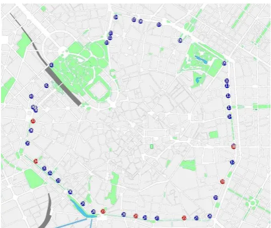
Area C has 43 access points each controlled by a video camera (Figure 6). Seven of them are dedicated exclusively to public transport. Video cameras detect the passage of vehicles

[image:9.595.133.463.384.579.2]

entering only and by reading license plates (as the charging fare allows free circulation within the area and multiple entries). A central system then recognizes the vehicle type, owner and charge due. It also provides information for fines or sanctions as needed.

(10)

[image:10.595.109.490.65.269.2]

a) b)

Figure 4: The whole network of Milan with roads classified by colours according to link capacity (4a) and with the “Cerchia dei Bastioni” area in red (4b).

a) b)

[image:10.595.107.491.307.513.2]

(11)

[image:11.595.163.432.59.285.2]

Figure 6: Locations of controlled points for accessing Area C.

The information available includes current traffic demand and public transport performance. Demand is represented by O/D (Origin/destination) matrices for the entire city and for the Bastioni. The latter is a smaller part of the inner centre of the City of Milan network where the charging is applied. These matrices are the result of calibration work undertaken by the AMAT agency since 2005 when a large survey on Milan and neighbouring municipalities was carried out. The number of centroids is 829 for the entire city network and 164 for the

Bastioni network. Matrices are split into five classes: cars, motorcycles, light trucks, heavy trucks and taxes. It should be noted that heavy trucks are not allowed to enter Area C.

Therefore for the Bastioni network, the network used for all the simulations presented in this paper, there are only four matrices based on the remaining modes. Assignment to the network was carried out using Cube Voyager (the software also used by AMAT), which performed a deterministic multiclass assignment to the Bastioni network.

The current charging policy is represented by the base level of demand in the study, i.e. the reference scenario. In order to assess the effect of changes to the charging scheme that could be considered instead, demand is changed by firstly reducing demand in steps of magnitude, and secondly by consideration of the possibility of an increase in demand. Area C is not a very large area and therefore a reasonable assumption was made that demand changes uniformly for links within this area.Scenarios were built for the Bastioni network using changing demand under two scenario types. These firstly represented changes in the charging scheme for a subset of the traffic mix (the Main Scenarios) and secondly, changes in charging for all vehicles (Secondary Scenarios):

- Main Scenarios: these were constructed by changing the demand for cars and light trucks only, as motorcycles do not pay. Taxis pay a reduced charge, but this is included in their fare and paid by clients - a demand class generally less sensitive to price. Scenarios were defined by reducing or increasing demand by the same

percentage for all O/D pairs. The particular percentages used were 10%, 40%, and -70% (coefficients 0.9, 0.6, and 0.3) in order to represent an increasingly steep

(12)

variations in cars and light trucks correspond to changing the whole demand by -2.3%, -8.9%,, -15.6% and +2.2% respectively. It is worth noting that when the current charging policy was introduced for Area C, the reduction in traffic entering into Area C in the first six months was around 34%. The exploration of variations in demand here include one change that would be of a similar size to this original impact (-40% demand), one which would represent a much higher additional charge and demand reduction (-70%), and two others that represent more marginal changes compared with the current scheme.

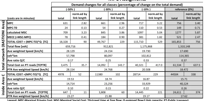
- Secondary Scenarios: these were created by changing the entire demand to see whether a different structure (i.e. different combinations of O/D pairs) would change the results or not. Scenarios were obtained by changing demand by a percentage of -10%, -30%, and -50% (coefficients 0.9, 0.7, and 0.5).

5. RESULTS AND DISCUSSION

5.1 Cost of congestion modelling analysis

Tables 1 to 4 report the results from the assignment of demand according to the scenarios described in the previous section. Table 1 and Table 2 refer to those scenarios where only the demand for cars and light trucks changes and they are divided according to the type of assignments, MPC or MSC. Table 3 and Table 4 refer to those scenarios where the whole demand changes (so that every class of demand changes by the same percentage).

The tables report results for: both the entire area of Bastioni and only for Area C and for both all roads and only for those roads shared with Public Transport. The variables are:

 the sum of Marginal Private Costs (MPC);

 the difference between MPC and T0, the free flow travel time (MPC-T0). This identifies the component of travel time due to congestion;

 the sum of calculated or assigned Marginal Social Costs (MSC);

 the total costs spent in the network due to congestion [(MPC-T0)*Q] where Q is the assigned link flow;

 the total costs of EBC;

 the ratio between total costs of EBC and the total cost of congestion;  the sum of assigned link flows (Total flow);

 the average speed weighted on flow;

 the product between the number of vehicles and travelled kilometers (veh*km);  the ratio Q/C where C is the link capacity; this value can be used to calculate the LOS

of the network.

(13)

(14)

Table 1: Main Scenarios : Marginal Private Cost Assignments by changing vehicles and light trucks demand only.

(costs are in minutes) total

norm.ed by

link length total

norm.ed by

norm.ed by link length

MPC 691 3.09 714 3.20 746 3.36 756 3.40 767 3.46

MPC-T0 84 0.40 107 0.51 139 0.66 149 0.71 160 0.76

calculated MSC 985 4.47 1089 4.97 1234 5.66 1277 5.87 1328 6.12

MECC (=MSC-MPC) 293 1.38 374 1.77 487 2.31 521 2.47 561 2.66

TOTAL COST = (MPC-TO)*Q [TC] 91,102 410 116,967 530 154,509 704 165,853 756 179,039 817

Total flow [veh]

Ave weighted Speed [km/h]

veh*km Ave ratio Q/C

Total Cost on PT roads [TCPTR] 28,172 287.8 39,430 406.5 55,944 579.9 61,534 637.5 68,115 707.2

PTR Ave weighted Speed [km/h]

TOTAL COST =(MPC-TO)*Q [TC] 16055 134 25032 199 39123 301 44504 338 50770 382

Total Cost on PT roads [TCPTR] 7,407 116 12,833 198 21,354 326 24,611 374 28,359 431

Legend: MPC-Marginal Private Cost; MSC-Marginal Social Cost; T0=travel time at free flow; Q-assigned flow;C-link capacity; PT-Public transport

15.71 15.27 17.10 to ta l n e tw o rk ( B A S T IO N I A re a ) 0.30 0.33

(-10% / -2.23%) reference (0% / 0%) (+10% / +2.23%)

MPC Assigments

(-70% / -18.55%) (-40% / -10.60%)

Demand changes only for Auto and Light Trucks classes (percentage of change for classes / on the total demand)

18.111 17.690 17.233

21.167 19.737 18.41 17.39 22.199 20.686 0.37 0.38 16.13 40,124 41,642

1,284,234 1,310,148 1,338,794

18.472 17.934

1,091,396 1,183,166

18.966

95,553 103,435 112,084 114,365 116,815

0.36 in si d e A re a C 17.62

20.83 19.59 18.09

38,658

0.19 0.22

29,026 33,677

(15)

[image:15.842.78.771.99.510.2]

Table 2: Main Scenarios: Marginal Social Cost Assignments by changing vehicles and light trucks demand only.

norm.ed by

MPC (at assigned MSC) 679 3.03 702 3.14 732 3.28 743 3.33 754 3.39

MPC-T0 72 0.33 95 0.44 125 0.59 136 0.64 147 0.69

caluclated MSC 923 4.161 1022 4.63 1159 5.28 1204 5.50 1254 5.74

MECC (=MSC-MPC) 244 1.13 320 1.50 426 2.00 461 2.16 500 2.35

TOTAL COST MECC*Q' 60,438 22 81,836 30 113,342 41 124,017 45 136,155 50

TOTAL COST of Excess Burden (TCEB) 16,883 77 19,499 90 22,891 106 23,353 108 23,957 111

Ratio TCEB / TC

Total flow (at assigned MSC) [veh]

Ave weighted Speed [km/h] veh*km

Ave ratio Q/C

Total Costs of Excess Burden on PT roads

[TCEBPTR] 3,789 38 4,724 48 5,778 58 5,959 59 6,288 61

Ratio TCEBPTR / TCPTR

TOTAL COST of Excess Burden [TCEB] 1,499 19 1,986 23 2,829 32 2,969 33 3,238 35

Ratio TCEB / TC

Total Cost of Excess Burden on PT roads -223 -3 -29 -1 406 4 489 5 683 8

Ratio TCEBPTR / TCPTR

0.167 0.148 0.141 0.134

0.072 0.067 0.064

0.097 0.092

0.30 0.31 0.32

0.120 0.103

Demand changes only for Auto and Light Trucks classes (percentage of change for classes / on the total demand)

(-70% / -18.55%) (-40% / -10.60%) (-10% / -2.23%) reference (0% / 0%) (+10% / +2.23%)

in si d e A re a C 0.23 0.27 14.438 12.731 -0.030 -0.002 15.71 13.74 0.093 0.079 to ta l n e tw o rk ( B A S T IO N I A re a ) 0.32 0.35 14.32 12.57 96,980 105,322 15.475 0.185

11.000 10.446 9.907

10.77 10.29 9.80

114,476 117,066 119,632

1,373,958

1,114,302 1,210,659 1,314,909 1,344,273

46,968

10.199

13.449 11.371 10.783

0.38 0.39 0.40

MSC Assigments

0.135

11.79 11.18 10.61

50,106 48,581

36,699 41,642

(16)

Table 3: Secondary scenarios: Marginal Private Cost Assignments by changing the total demand.

norm.ed by

MPC 631 2.82 661 2.96 717 3.22 756 3.40

MPC-T0 24 0.13 54 0.27 110 0.53 149 0.71

calculated MSC 709 3.23 845 3.86 1097 5.04 1277 5.87

MECC (=MSC-MPC) 78 0.41 184 0.90 381 1.82 521 2.47

TOTAL COST = (MPC-TO)*Q [TC] 18,328 90 49,767 229 115,710 529 165,853 756

Total flow [veh]

Ave ratio Q/C

Total Cost on PT roads [TCPTR] 3,475 35.7 14,092 143.7 40,321 417.0 61,534 637.5

TOTAL COST =(MPC-TO)*Q [TC] 4978 52 11380 102 28714 229 44504 338

Ave ratio Q/C

Total Cost on PT roads [TCPTR] 647 11 3,808 60 14,445 221 24,611 374

17.62 0.26 40,124

80,097 102,812 114,365

15.71

in

si

d

e

A

re

a

C

19.53 18.74 16.87

14,714 23,256 33,929

0.10 0.15 0.22

23.27 21.88 19.17

MPC Assigments

Demand changes for all classes (percentage of change on the total demand)

(-50% ) (-30% ) (-10% )

17.690 reference (0%)

to

ta

l

n

e

tw

o

rk

(

B

A

S

T

IO

N

I

A

re

a

)

659,716 912,821 1,175,868 1,310,148

28.129 24.154 19.730

0.37

28.154 24.768 20.508 18.472

0.17 0.25 0.33

[image:16.842.75.774.114.462.2]

57,798

(17)

[image:17.595.128.468.70.250.2]

Figure 7: Q/C (flow/capacity) ratio distribution histogram (MPC assignment – demand changes only for cars and light trucks).

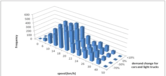
Figure 8 : Distribution of Average Link Speed (MPC assignment – demand changes only for cars and light trucks).

In Figures 7 to 12, distributions of flow capacity ratio, link speed and EBC are reported for the main scenarios. From Figure 7 it can be seen that as demand increases, the flow/capacity ratio generally increases as might be expected. The largest changes are seen with increases in demand of 0.6 or more, with noticeable changes in the number of links reaching saturation. A corresponding decrease in links with very low Q/C ratio is illustrated at the opposite end of the axis.

[image:17.595.122.474.283.445.2]

(18)

[image:18.595.111.488.72.195.2]

a) b)

Figure 9 : Distribution of Excess Burden of Congestion in Bastioni area (9a) and only for PT roads (9b) (demand changes only for cars and light trucks).

a) b)

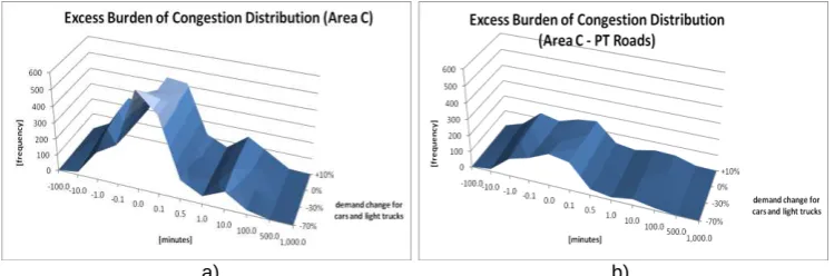
Figure 10 : Distribution of Excess Burden of Congestion in Area C (10a) and only for PT roads (10b) (demand changes only for cars and light trucks).

A comparison between Figure 9 and Figure 10 highlights the difference between changes in EBC for Bastioni and Area C as demand increases. The EBC for Bastioni is seen to

demonstrate a more gradual reduction, whilst increased demand has a noticeably greater impact on the values of EBC for Bastioni than for Area C. The main difference between the two sites in practice is that Area C excludes the ring roads that are included in the scope of the Bastioni region. There may be a number of factors that contribute to the distributions overall, but referring back to Figure 4, some high capacity parts of the network are not included in Area C which may offer greater flexibility and some additional capacity to absorb extra demand – at least for the moderate increases in demand. The standard deviation of EBC is lower inside Area C than it is in Bastioni, and for PT roads (in this case its value is about half that for all roads).

5.2 Ex-post travel time analysis

[image:18.595.111.486.246.370.2]

(19)

[image:19.595.90.511.132.643.2]

Ecopass (year 2011) are about 32.8% and 31.2% respectively. It must be emphasised that the average values of percentages are calculated on the row data (and not as the ratio of the final average values).

Table 5: Average speed [km/h] summary for Public Transport links and lines in Milan (Area C and the whole city)

time 8:00-09:59

year 2011-2012 2011 (A) 2012 (B) %(B-A)/A 2011 (A') 2012 (B') %(B'-A')/A'

ave 10.77 10.63 10.98 3.98 10.43 10.80 4.93

dev.std 3.45 3.48 3.56 11.84 3.53 3.51 15.89

ave 10.04 10.09 10.49 4.63 9.57 10.20 9.07

dev.std 3.35 3.43 3.49 13.09 3.41 3.44 23.33

time 8:00-09:59

year 2011-2012 2011 (A) 2012 (B) %(B-A)/A 2011 (A') 2012 (B') %(B'-A')/A' ave 9.40 9.25 9.51 1.53 8.76 9.27 6.15

dev.std 2.03 1.99 2.31 8.68 2.18 2.15 11.95

ave 7.95 8.06 8.19 0.52 7.63 8.11 9.74

dev.std 1.79 1.30 1.74 10.44 2.01 1.82 16.22

ave 10.42 10.44 10.84 2.24 _9.88 _10.44 3.61

dev.std 1.52 1.87 2.07 7.46 1.78 1.84 7.24

time 8:00-09:59

year 2011-2012 2011 (A) 2012 (B) %(B-A)/A 2011 (A') 2012 (B') %(B'-A')/A'

ave 17.62 16.88 17.15 3.06 _17.28 _17.64 3.13

dev.std 7.33 7.03 7.16 20.91 7.23 7.83 29.37

ave 15.77 15.31 15.45 3.20 15.72 16.05 4.31

dev.std 6.62 6.60 6.44 24.83 6.77 6.88 26.96

time 8:00-09:59

year 2011-2012 2011 (A) 2012 (B) %(B-A)/A 2011 (A') 2012 (B') %(B'-A')/A'

ave 14.79 13.42 13.54 1.09 11.24 11.72 3.10

dev.std 4.11 3.65 3.62 7.23 4.86 4.80 11.95

ave 10.41 10.53 10.76 1.94 10.15 10.54 5.04

dev.std 1.40 1.22 1.51 5.52 1.86 1.56 9.79

ave 15.49 14.72 14.78 0.71 15.52 15.72 2.13

dev.std 3.96 3.64 3.61 7.94 4.92 4.95 12.96

ON LINES (on time) ON LINKS ON LINES (on time) ON LINKS Area_C City 9:00 8:00 9:00 number of lines number of lines 9:00 8:00 9:00 8:00 8:00 number of links number of links All Tramway Bus ( on speed)

(on time)

( on speed)

(on time) Tramway All Bus 123 17 106 284 284 29 12 17 5261 5261 8.0 9.0 10.0 11.0 12.0 13.0 14.0 15.0 16.0 17.0

2011 2012 2011 2012

sp e e d [ k m /h ] year

Link average speed

H8:00 H9:00 AREA C City +4.63% +9.07% +4.31% +3.20%

Figure 11 :Comparisons between average (time) speed on links before (2011) and after (2012) the introduction of charging both for Area C and the entire City.

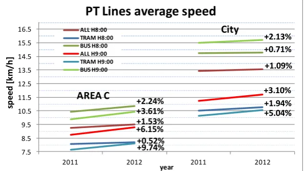
[image:19.595.84.511.144.440.2]

(20)

infer a specific effect from charging. The effect is more evident for the 9:00 time segment than 8:00, and for links than for lines. Bus mode seems to achieve higher benefits from charging than the tram mode.

7.5 8.5 9.5 10.5 11.5 12.5 13.5 14.5 15.5 16.5

2011 2012 2011 2012

sp e e d [ k m /h ] year

PT Lines average speed

[image:20.595.150.449.121.288.2]

ALL H8:00 TRAM H8:00 BUS H8:00 ALL H9:00 TRAM H9:00 BUS H9:00 AREA C City +2.24% +3.61% +1.53% +6.15% +0.52% +9.74% +0.71% +1.09% +2.13% +3.10% +5.04% +1.94%

Figure 12: Comparisons of average speed on Public Transport lines before (2011) and after (2012) introduction of charging both for Area C and the entire City.

6. CONCLUSIONS

The objectives of the study were to consider how the costs of congestion may vary with policy-related demand changes around the city of Milan. The demand change scenarios effectively represent hypothetical variations in the charge within the so-called Area C scheme

– a subarea at the heart of the Bastioni sector, which is itself a part of the wider Milan city. The demand variations were introduced within two main scenarios, representing charging variations for a subset of vehicles and for the whole traffic respectively. The levels of demand change were set with consideration to the size of demand change observed when the Area C scheme was first introduced. In summary, these represented a marginal further demand change (+ or – further 10%), a further equivalent decrease in demand (-40%, roughly

comparable with the -34% observed) and finally a significant demand reduction (-70%). Two measures for the costs of congestion were calculated – one being an estimate of the total cost of congestion (TCC) and the second being the excess burden of congestion (EBC). These were calculated for both the immediate Area C region and the wider Bastioni sector in order to explore possible shifts in costs. Other traffic related measures relating to speeds were also calculated. The study has generated some interesting insights and has produced a series of questions for further study, with the main findings as follows:

 A strong correlation is seen between the cost of congestion measures and vehicle speeds (r = 0.98) ; this is not surprising since speed (v) and cost (c ) are related by a

relationship of the form of v≈1/c for each link. This does, however, lead to the

conjecture that speeds may be used as a proxy for the costs of congestion, a phenomena that is worth further future study;

 From the two measures for the costs of congestion considered, it can be seen that the Total cost of congestion is much higher than EBC (EBC is between 13% and 18% of TCC for main scenarios). However the Total cost falls more quickly than EBC as the cordon charges increase (demand reduces). At low levels of demand EBC is almost one fifth of TCC, whilst at higher demand levels it is closer to a tenth. This raises the

(21)

measures and the need for careful policy interpretation of each of the two measures in practice;

 Sub-optimal conditions can occur on certain parts of the network even though the network is moving towards a more optimal position (from a congestion perspective). This is evidenced by the fact that for some links EBC can be negative. It is attributed to particular characteristics of cordon charges, one way systems and PT only links. It is worth noting that what may be viewed as sub-optimal conditions in terms of congestion and system efficiency may be perceived as very acceptable and even positive conditions from the perspective of some stakeholder groups (for example residents or regular

commuters with ‘rat-running’ behaviours);

 Finally, a travel time (speed) analysis was carried out by way of ex-post analysis of the impact of introducing the Area C scheme (representing the change in demand of -34% compared with the previous charging scheme, Ecopass). The changes in demand in Area C are clearly not entirely independent of the whole city, although the conditions at the whole city level could be considered as an approximate comparison group. For the whole city, an increase in traffic speeds is seen for both links and lines (PT). However, the increase in speed is more marked for Area C than for the whole city, reflecting the immediacy of the impacts around the direct locality of the charging policy. The effect is more evident at 9:00 than 8:00, and for links than for lines.

A number of topics for further research have arisen alongside the main research findings:  A more elaborate set of scenarios could (in principle) be explored to look at the impact

of re-investing congestion charges back into the transport network (through improved PT or better circumferential road routes around a cordon, or a form of active traffic management using ‘intelligent transport’ schemes;

 Further analyses that separates the data into city segments or main route roads vs the remainder would be interesting in order to calculate some simple measures around equity in terms of distribution of impacts. Research (in collaboration with the city

authority) could involve identification of which particular areas, routes and ‘critical links’ are known to have policy issues or are otherwise of priority. Critical links may also emerge from further research concerning the influence of particular links on the overall indexes. As can be seen from Figure 7, not many critical links may be present in the network though. These could then be studied in more detail for either an equity analysis or for more in-depth knowledge of other impacts of the charging policy.  A more in-depth study should consider the network design issue – this relates to the

presence of one way streets, regulatory restrictions on traffic in particular areas and possibly planning/engineering issues around road width or quality that impact on route choices and traffic flow. It is conjectured that these types of factors may be underlying the presence of some negative EBCs in the cost calculation. A set of wider

considerations may be included in such a study such as the impacts on particular sub-groups or sub-areas of the study region, who may perceive particular positive

advantages from the current network design;

(22)

AKNOWLEDGEMENTS

Thanks are due to the Mobility, Environment, Territory Agency of Milan (AMAT) who provided data for the research.

REFERENCES

AMAT, 2008. Origin/Destination matrixes. http://www.amat-mi.it/it/documenti/dettaglio/17/. Barth, K,, Boriboonsomsin, K., 2008. Real-world carbon dioxide impacts of traffic congestion.

Transportation Research Record, Record n.2058, 163-171.

Bilbao-Ubillos, J., 2008. The costs of urban congestion: Estimation of welfare losses arising from congestion on cross-town link roads. Transportation Research Part A: Policy and Practice, Vol. 42 (8), pp. 1098–1108.

Brownfield, J, Graham, A:, Eveleigh, H, Ward, H., Robertson,, S., Allsop, R., 2003. Congestion and accident risk. Road Safety Research Report No. 44, DfT. http://www.dft.gov.uk.

Button, K., 1993. Transport Economics. 2nd Edition, Edward Elgar, Aldershot

City of Stockholm, 2005. Information Brochure: On Stockholm’s Trial, English Version.

Dodgson, J., Young, J., van der Veer, J., 2002. Paying for Road Use, Technical Report, A report to the Commission for Integrated Transport, National Economic Research Associates (NERA), London, February. Available online at: http://www.cfit.gov.uk/ docs/2002/pfru/research/pdf/pfru-tech.pdf accessed 27th October 2012.

European Commission, (2011) WHITE PAPER Roadmap to a Single European Transport Area – Towards a competitive, and resource efficient transport system, available online http://eur- lex.europa.eu

Glaister, S. , 1981. Fundamentals of Transport Economics. Basil Blackwell, Oxford.

Goodwin, P.B., 2004. The Economic Costs of Road Traffic Congestion. Discussion paper. Rail Freight Group, Transport Studies Unit, University College London. http://eprints.ucl.ac.uk/archive/00001259/.

Grant-Muller, S.M., Laird, J.J., 2007. The Cost of Congestion. European Transport Conference, Noordwijkerhout 17-19 October 2007. London: AET Transport.

Highways Agency, Scottish Office development department, The Welsh Office, The department of the Environment for Northern Ireland, 1997. Design manual for Roads and Bridges, Traffic Flow Ranges for Use in the Assessment of New Rural Roads. DMRB, Vol 5, Section1, Part 3. http://www.highways.gov.uk/.

Lindberg, G., 2006, Marginal cost case studies for road and rail transport. Deliverable D 3, GRACE. Funded by Sixth Framework Programme. ITS, University of Leeds, Leeds, November 2006. Available online at: http://www.grace-eu.org/deliverables.htm accessed 27th October 2012.

Marfia G., Roccetti, M., 2011. Vehicular Congestion Detection and Short-Term Forecasting: A New Model with Results. IEEE transactions on vehicular technology, vol. 60, no. 7, pp. 2936 – 2948.

Mayer, C., Sinai, T., 2003. Network effects congestion externalities and air traffic delays: or why not all delays are evil. American Economic Review 93 (4), pp.1194-1215.

(23)

Moran, C., Koutsopoulos, H., 2010. Congestion indicators from the users’ perspective: alternative formulations with stochastic reference level. In12th World Conference on Transport Research.

Newbery, D.M., 1990. Pricing and Congestion: Economic Principles Relevant to Pricing Roads. Oxford Review of Economic Policy, Vol 6 (2), pp. 22-38.

Sheffy, Y., 1985. Urban transportation networks. Prentice-Hall, Inc., Englewood Cliffs, N.J. Shy, O., 2001. The Economics of Network Industries. Cambridge University Press:

Cambridge.

Van Vliet, D., 1982. SATURN - A Modern Assignment Model. Traffic Engineering and Control, vol 23, Issue 12, Publisher: Hemming Group, Limited, ISSN: 0041-0683. Waadt, A., Wang, S., Bruck, G., Jung, P., 2009. Traffic congestion estimation service

exploiting mobile assisted positioning schemes in GSM networks. Procedia Earth and Planetary Science, Special issue title: Proceedings of the International Conference on Mining Science & Technology (ICMST2009), Eds Shi-rong Ge, Jiong-tian Liu and Chu-wen Guo, Vol. 1 (1), pp. 1385–1392.

Walters, A., 1961. The Theory and Measurement of Private and Social Cost of Highway Congestion. Econometrica, 29, 676-99.

APPENDIX A: GLOSSARY

EBC = Excess Burden of Congestion

MECC = MSC – MPC = Marginal Social Costs minus Marginal Private Costs MPC = Marginal Private Costs

(MPC-T0)*Q = Total Costs spent in the network due to congestion, Q is the assigned link flow

MSC = Marginal Social Costs PT = Public Transport

PTR = Public Transport Roads

Q/C = Ratio between the assigned link flow, Q, and the link capacity, C TC = Total Costs