Experimental quantification of contaminant ingress into a buried leaking pipe during transient events

Experimental Quantification of Contaminant Ingress into a

Buried Leaking Pipe during Transient Events

Sam Fox

; Will Shepherd, Ph.D.

; Richard Collins, Ph.D.

; and Joby Boxall, Ph.D.

Abstract:It has been hypothesized that negative pressures caused by transients within water distribution systems may result in ingress of

contaminated groundwater through leaks and hence pose a risk to public health. This paper presents results of contaminant ingress experi-ments from a novel laboratory facility at The University of Sheffield. An engineered leak surrounded by porous media was subjected to pressure transients resulting from the rapid closure of an upstream valve. It has been shown that a pollutant originating externally was drawn in and transported to the end of the pipe loop. This paper thus presents the first fully representative results proving the occurrence and hence, risk to potable water quality of contaminant ingress.DOI:10.1061/(ASCE)HY.1943-7900.0001040.This work is made available under the terms of the Creative Commons Attribution 4.0 International license,http://creativecommons.org/licenses/by/4.0/.

Author keywords:Pressure transient; Contaminant ingress; Water quality; Leakage.

Introduction

Water suppliers are responsible for continuously supplying clean and safe drinking water fundamental to society and public health and well being. Potential impacts of failing to adhere to this obli-gation include economic repercussions, but significantly, the risk posed to public health. Losses from leaks and bursts, are a well-documented issue within water distribution systems (WDS), which impact both customers and suppliers. In England and Wales the average reported levels of leakage for 2009–2010 were estimated at 131 L per property (Ofwat 2010). Phenomena in WDS that are less well understood are pressure transients, which can result in negative pressures (Gullick et al. 2004). The coexistence of nega-tive pressures and leaks in distribution systems means there is a risk of contaminant ingress. Such ingress could result in possible inci-dents of water quality deterioration and a failure to meet prescribed standards (Lechevallier et al. 2003). A U.K. study (Hunter et al. 2005) into self-reported diarrhea in a control group found a strong association between reported cases of diarrhea and low pressures at consumer taps. The investigation provided a feasible assertion that the presence of low pressures within distribution systems is asso-ciated with public health, likely due to contamination events.

While it is generally accepted that negative pressures can result in ingress from surrounding groundwater, there is a perception that, due to the short duration, oscillating nature of pressures transients, only water that has been expelled from the distribution system will reenter the pipe or that if contaminant is intruded it will be expelled

on the next positive pressure cycle. In order to ascertain if a contaminant originating externally to a pressurized pipeline can be intruded and remain within the pipeline, thus posing a risk to water quality, an innovative physical investigation was designed and implemented. The work presented here aims to explore via fully representative, but extreme, physical experiments whether a contaminant originating externally to a pressurized pipeline can be intruded and remain within the pipeline.

Contaminant Ingress

Lindley and Buchberger (2002) define the three requirements that must coexist for contaminant ingress to take place within water dis-tribution systems; the existence of a contaminant source external to the distribution pipe, a pathway providing a route into the system, and a driving force.

Contaminant Source

An American Water Works Association Research Foundation sponsored study (Kirmeyer et al. 2001) identified and quantified pathogens occurring in the ground surrounding mains water pipes. Within the investigation, researchers collected soil and water samples external to existing water pipelines from six different U.S. states and tested for a range of microbial indicators and vi-ruses. Results of the study showed that 50% of the soil samples tested contained fecal coliforms in addition to the identification of other bacterium and viruses within the samples. Whereas iso-lated nonreplenishable contamination events create a potential environment for contaminant ingress to occur, continuously re-newed contamination sources such as a leaking sewer above a failed mains distribution pipe, as presented by Karim et al. (2003), increase the likelihood of the occurrence of this phenome-non. The risk posed by contaminants, in both solute and particulate form, is further magnified due to the widespread existence of biofilms within water distribution systems which may provide shelter and a platform for such pathogenic bacteria and viruses to multiply (Eboigbodin et al. 2008). Contaminant ingress may therefore result in direct exposure to customers and/or less direct risks such as seeding of biofilms.

1_{Pennine Water Group, Dept. of Civil and Structural Engineering, Univ.}

of Sheffield, Mappin St., Sheffield S1 3JD, U.K. (corresponding author). E-mail: [email protected]

2_{Pennine Water Group, Dept. of Civil and Structural Engineering,}

Univ. of Sheffield, Mappin St., Sheffield S1 3JD, U.K.

3_{Pennine Water Group, Dept. of Civil and Structural Engineering,}

Univ. of Sheffield, Mappin St., Sheffield S1 3JD, U.K.

4_{Professor, Pennine Water Group, Dept. of Civil and Structural}

Engineering, Univ. of Sheffield, Mappin St., Sheffield S1 3JD, U.K. Note. This manuscript was submitted on April 2, 2014; approved on March 30, 2015; published online on July 8, 2015. Discussion period open until December 8, 2015; separate discussions must be submitted for

indi-vidual papers. This paper is part of theJournal of Hydraulic Engineering,

© ASCE, ISSN 0733-9429/04015036(10)/$25.00.

Pathway

Pathways through which external contaminant may enter the dis-tribution system exist in various forms. Kirmeyer et al. (2001) ranked the potential routes of entry (pathways) into the distribution system based on the associated risk level. Water treatment break-through and water main breaks were among the highest risk path-ways, with new main installation and purposeful contamination events ranked as low risk. Failures in the integrity of distribution pipes resulting in a system leak are therefore classed as high risk routes of entry. Examples of typical leak types in water distribution system pipes are pin holes, cracks, corrosion clusters, and joint/ connection failures (Clayton and van Zyl 2007). Another potential pathway particularly relevant to low pressure and transient events is through air valves when the chamber in which they are located becomes flooded (Ebacher et al. 2012).

Driving Force

Fluids will always flow from high to low pressures, thus when the pressure within a pipe drops below the local groundwater pressure, a potential driving force for contaminant ingress exists. Longer term depressurization due to maintenance/repair work may therefore result in the formation of such conditions leading to steady-state intrusion (Collins et al. 2012b). The differential pressures required for intrusion into WDS can also result from the presence of negative pressure transients within a system.

Water industry data regarding pressures in WDS is typically re-corded at 15 min intervals. This is a good measure of daily trends and patterns, but also provides an artificially smooth representation of the system characteristics leading to an assumption that the pres-sures are approximately steady. Observations from field studies re-ported on the occurrence of pressure waves, in a series of locations in two separate systems, recorded using high speed pressure data loggers confirming the occurrence of transients within operational systems (Kirmeyer et al. 2001). A qualitative comparison of the influence data sampling rates have on the perceived steadiness of system pressures was presented by Fox et al. (2013) with high frequency data from live distribution systems demonstrating the complex and dynamic nature of the hydraulic conditions within WDS. As part of a larger data logging exercise, Starczewska et al. (2013) presented two case studies highlighting the occurrence of pressure transients within complex distribution networks. The re-searchers identified the source of the transients as the pump feeding the region, with the transient data aligning with the pump switching (on and off).

Dynamic pressure conditions occur due to a rapid change in the water velocity, which may be a result of operational changes in-cluding valve closures, system depressurization for maintenance work and changes in demand, or due to asset failures such as pump trips and bursts (Collins et al. 2012b). These extreme changes of flow within the system incur the risk of oscillating high and low pressure transients, where the lowest pressures may be negative (Brunone and Ferrante 2004;Gullick et al. 2004). Low and neg-ative pressures are most likely to occur downstream from an im-posed obstruction (e.g., valve closure) where the momentum of a flowing column of water may result in the formation of low or negative pressures bounded at water vapor pressure (Ghidaoui et al. 2005). The greater the initial velocity of the body of fluid the more extreme the negative pressure wave formed following a sud-den change in flow conditions. Along with the previously discussed risk of contaminant ingress and the subsequent water quality issues, there is also a recognized threat to the structural integrity of the system from extreme transient pressures.

Quantifying the Risk of Ingress

Researchers have adopted different approaches to quantifying the risk of contaminant ingress into water distribution systems. Statistical analysis techniques have been used (Sadiq et al. 2006; Deng et al. 2011) as well as field (Ebacher et al. 2012) and exper-imental studies aimed at improving the understanding of the mechanism of contaminant ingress in order to better define the as-sociated risk. At its simplest the physical risk of contaminant intrusion, according to reasonable engineering judgment, may be considered greatest when the external contaminant is above or di-rectly in the line of the leak jet (providing the shortest pathway along a flow route into the orifice).

Experimental work to quantify the intrusion magnitude through leak orifices under steady state (L´opez-Jiménez and Mora-Rodríguez 2010;Collins et al. 2012b) and dynamic pressure con-ditions (Boyd et al. 2004;Collins et al. 2011a; Mora-Rodríguez et al. 2011) provide a greater understanding to this phenomena, in particular the influence of porous media surrounding a failed pipe. Collins and Boxall (2013) derived and fully validated an ana-lytical model, improving on the standard orifice equation, to define the flow into a system through a failure aperture in a pipe buried in porous media subject to steady-state conditions. Furthermore, work to quantify the pressure-dependent behavior of different failure types in pressurized distribution mains (Fox et al. 2012;van Zyl and Cassa 2014) and the continual evolution in the reliability and accuracy of transient modeling techniques provide a platform to better understand and mitigate the risk of ingress of contaminants within WDS.

The experimental research presented here aims to build upon and develop the understanding of the physical process of contam-inant intrusion in order to better define the threat posed to water quality in real networks. Ultimately this paper seeks to prove or otherwise if a contaminant originating externally to a pressurized pipe can be intruded into, remain within and be transported.

Experimental Methodology

A large-scale and fully representative laboratory facility has been constructed at the University of Sheffield to investigate pressure transients, leakage and particularly the various factors associated with the potential for contaminant ingress into distribution systems. The general features of this facility are described in the laboratory facility section, with the specific configuration for determining whether external contaminants can be ingressed into the pipe, de-tailed in the ingress configuration section.

Laboratory Facility

The contaminant ingress in distribution systems laboratory facility is a recirculating pipe system; a schematic of the system is shown in Fig.1. The 141 m length facility is constructed from 63 mm diam-eter (nominal internal diamdiam-eter of 50 mm, SDR 11) medium density polyethylene (MDPE) pipe produced by GPS PE Systems (Huntingdon). The system consists of seven loops that are sup-ported and restrained by 16 stands mounted on footings integral to the concrete slab floor. The system has an oval plan form with the pipe always rising to facilitate air removal. Water is fed into the system from a single upstream reservoir (holding tank) and returns to this same tank, with a maximum capacity of 1,080 L, by a 3.5 kW Wilo MVIE variable speed pump (WILO, Staffordshire, U.K.) (range 1,000–3,380 rpm). Quarter turn butterfly valves, located at itemsc,f, andjin Fig.1, allow for the isolation of differ-ent sections of the pipe loop including the test box section (h). The

flow conditions (pressure head and system flow rate) are controlled by the pump speed and a single downstream globe control valve (k). Gems 2200 series pressure sensors (Gems Sensors, Basing-stoke, England) located ate,g, andiwere used to record the pres-sure heads whereas the system flow rate was meapres-sured using an Arkon Flow System Mag-900 electromagnetic flow meter (Arkon Flow Systems, Brno, Czech Republic) located immediately down-stream from the pump (d). Data was logged at 300 Hz using National Instruments’ LabVIEW software (National Instruments Corporation, Berkshire, U.K.) and a measurement computing PMD1820 data acquisition device (DAQ) (Measurement Comput-ing Corporation, Norton, Massachusetts).

Ingress Configuration

A test section box (total volume of 458 L), itemhin Fig.1, housed a 0.8 m length test section pipe containing a single engineered 5 mm diameter circular orifice facing horizontally. An overflow weir at the top of the box (0.45 m above the pipe center line) pro-vided a means to maintain a constant water level during testing. The mean flow rate through the leak was obtained by collecting the water from the weir in an isolated collection tank and measuring the volume increase over time. The test section was manufactured from the same specification pipe as the main loop, with flanges to secure the section 61 m downstream from the holding tank. The test section was buried under 0.45 m depth of mixed-grade pea gravel (approximately 5–12 mm diameter) consistent with the British Standard for backfill material for plastic pipework [British Standards Institution (BSI) 1973], with the leak orientated horizon-tally to minimize the movement of the gravel surrounding the pipe. Nonpreferential boundary conditions were ensured through the

addition of a green roof drainage lining for the box. A fine metallic mesh (wire diameter 0.5 mm, square grid at 2 mm centers) was affixed over the leak to ensure that no gravel entered the system during testing.

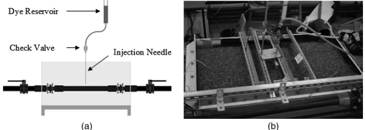
Rhodamine WT fluorescent dye, at a concentration of 1×10−3_{L=L, was used as a pseudo pollutant. An injection system} was used to create a discrete cloud of pollutant at selected locations around the leak. Fig. 2 shows the setup of the injection system which consisted of a dye reservoir, connected via a 6 mm internal diameter flexible tube to a check valve, to prevent backflow, and finally to a 1 mm hollow steel needle affixed to a structural support frame. The open end of the needle was positioned in the gravel at different locations relative to the leak, the location of the needle tip is defined using a Cartesian coordinate system. Thex,y, andzaxes refer to the horizontal distance parallel to the pipe, the horizontal distance perpendicular to the pipe and the vertical distance perpendicular to the pipe, respectively, with (0,0,0) representing the center of the leak. The structural support frame provided an accurate method for positioning the injection needle in preparation of each test and also ensured the needle was secured in place during the repacking of the gravel. A quarter-turn valve below the reservoir enabled a controllable and repeatable volume of dye to be injected for each test.

In order to quantify the volume of any pollutant ingressed into and net transported to the end of the system (rather than being ex-truded on the next positive cycle of the transient), a Turner Designs’ Cyclops 7 fluorometer (Turner Designs, Sunnyvale, California) was located 71 m downstream of the test section (itemlin Fig.1) and the output recorded using the PM1820 DAQ device also at 300 Hz. The fluorometer was located at the outlet, downstream of the control valve at a sufficient distance from the leak to ensure Fig. 1.Schematic of the contaminant ingress into distribution systems facility at the University of Sheffield

Fig. 2.(a) Cross section diagram of injection system and test section box; (b) experimental setup in the contaminant ingress in distribution system facility

that any rhodamine WT was cross-sectionally well mixed. A second fluorometer (item a in Fig. 1) was located upstream of the test section to record any variations in background concentration of rhodamine WT due to the recirculatory nature of the system. The chemical stability of the dye used ensured there was negligible concentration decay during the course of testing. The volume of ingressed pollutant was quantified by taking the integral of the measured dye concentration from the downstream fluorom-eter. Both fluorometers were installed at the edge of the pipe (essentially flush with the fluorometer head slightly convex whereas the inside of the pipe is concave) to minimize distortion of the flow.

Experimental Procedure

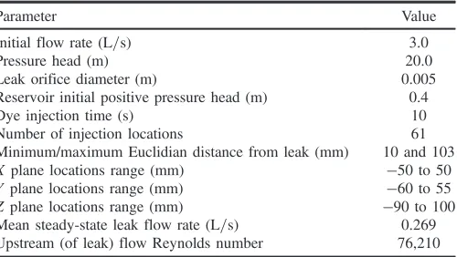
The accuracy and repeatability of the proposed experimental work was evaluated during a phase of preliminary testing, the results of which are discussed but not presented herein. Details of the devel-oped experimental parameters are listed in Table1. The maximum feasible range of injection locations, the significance of the degree of gravel packing on the leakage flow rate, and the influence of the fine mesh placed across the leak were assessed. It was shown that the packing of the gravel had no measurable effect on the leakage flow rate and that there was a negligible head loss through the mesh. Following the preliminary work, a procedure was finalized to ensure repeatable results were obtainable. A total of 61 injection locations (coordinates) were explored within the investigation, pro-viding a wide range of distances from the leak orifice in three-dimensional space to assess the zone of influence of the intrusion phenomena.

The tests were all conducted under fully turbulent flow condi-tions using the same initial pipe flow rate of3.0L=s, equating to a velocity of1.53m=s, and test section pressure head of 20.0 m. The pipe flow velocity is relatively high and the pressure head low but fully realistic when compared with the typical flows and pressures expected within WDS in the U.K. These extreme but realistic con-ditions (high flow velocity and low pressure) result in negative pressure transients following rapid valve closure. The pressure transients for the tests were generated by closing the quarter turn butterfly valve immediately upstream of the test section box (itemf in Fig.1). The repeatability of transient pressure generation in this manner was demonstrated in Collins et al. (2012a) and can also be seen in Fig.3. The valve closure time was less than the character-istic time of the system and was therefore assumed to be an instan-taneous valve closure.

The primary and subsequent pressure transients generated from a single test, where the injection location coordinates were (0,0,10), have been overlaid in Fig.3. This figure with a short time period view of the test section pressure trace shows the formation of the transient pressure waves following the instantaneous closure of the upstream butterfly valve. The traces show the approximate 1 s duration of the negative pressure head during the three oscillations. The minimum recorded pressure head was−10.04m (cavitation pressure, with correspondingflatcomponent of trace) with a maximum second peak of 16.8 m. The transient pressure waves dissipated within approximately 3.0 s. Statistical analysis of the comparison between the individual generated transients and the mean values, produced an average coefficient of determi-nation (R2) of 0.997 and an average root-mean-square error (RMSE) of 0.472 m over a 13 s time period showing that highly repeatable transients were generated.

Following accurately locating of the needle tip in the designated test location (1mm), the gravel was repacked around the needle and fully submerged under a constant depth of water. Initial steady-state hydraulic conditions were then set in the pipe loop and leak flow, and allowed to stabilize. Dye was then injected into the box for a period of 10 s, controlled by the manual operation of a single valve beneath the dye reservoir. A negative transient (primary transient) was generated 5 s after the start of the dye injection by closing the valve immediately upstream of the test box. Once the transient pressure wave within the system had dissipated the valve was opened and then closed twice more to generate a total of three negative pressure transients during the test (these repeated transients were generated to check for any secondary effects such as re-extrusion of contaminant). The two subsequent transients were generated without any additional injection to check for remaining dye solution in the porous media. The approximate 25 s time in-terval between each transient initiation allowed for the dissipation of the pressure wave and allowed approximate steady-state condi-tions to be reached before subsequent valve closures. The total vol-ume of dye injected into the test section tank was recorded by measuring the change in dye solution level within the reservoir (measurement error 0.015mL). For each of the point source pollutant locations, a minimum of three repeat tests were con-ducted. The background concentration of dye within the system was recorded using the fluorometer immediately upstream from the pump (item ain Fig. 1). During the analysis of the recorded data, this background concentration was removed to allow for the accurate calculation of the recovered volume of simulated pol-lutant ingress.

Table 1.Experimental Parameters As Defined within Test Planning and Procedure

Parameter Value

Initial flow rate (L=s) 3.0

Pressure head (m) 20.0

Leak orifice diameter (m) 0.005

Reservoir initial positive pressure head (m) 0.4

Dye injection time (s) 10

Number of injection locations 61

Minimum/maximum Euclidian distance from leak (mm) 10 and 103

Xplane locations range (mm) −50to 50

Y plane locations range (mm) −60to 55

Zplane locations range (mm) −90to 100

Mean steady-state leak flow rate (L=s) 0.269

Upstream (of leak) flow Reynolds number 76,210

−0.5 0 0.5 1 1.5 2 2.5 3 3.5 4 −20

−10 0 10 20 30

Time (s)

Pressure Head (m)

Primary Transient Second Transient Third Transient

Fig. 3. Overlaid pressure head traces from primary and subsequent generated transients during single test for point source pollutant injec-tion locainjec-tion (0,0,10)

Results

Qualitative Results

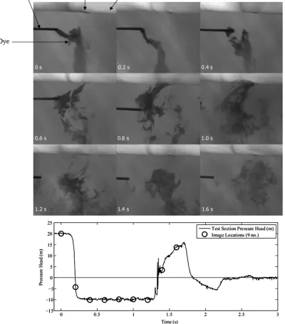
A qualitative demonstration of the phenomenon of contaminant ingress is depicted in the sequence of images shown in Fig. 4. An experimental setup equivalent to the aforementioned configu-ration, but without the inclusion of gravel in the test section box, was used to show the ingress of a representative point source pol-lutant during a single transient event. Rhodamine dye was injected external to the pipe leak contained in the water filled test section box. Dye injection was stopped after 1 s to facilitate observation of possible re-extrusion of contaminant. A clear correlation between the recorded pressure heads and the direction of the representative pollutant flow, away from or towards (and into) the leak orifice, may be observed. In addition, no re-extrusion of contaminant was noted within the recorded images.

Quantitative Results

Three examples of the results recorded from different point source locations are presented in detail herein. Fig.5is taken from a test where the representative point source of pollutant was injected at (0,0,10), i.e., 10 mm directly above the center of the leak orifice. Fig.5shows the recorded data from the test section pressure trans-ducer (solid line) approximately 1 m downstream of the leak (itemi in Fig.1), the injection start and stop time (dash-dot line), as well as the two fluorometer traces located upstream (dashed line) and downstream (solid line) of the leak. The start of the primary tran-sient has been assignedt¼0s (assumed instantaneous closure of the upstream valve).

The total injection volume over the 10 s injection period was measured at 7.4 mL and, as can be seen from the fluorometer trace, a peak concentration of1.35×10−7 L=L was recorded following the generated pressure transients. The recorded pulse equates to a Fig. 4.Sequence of images (0.2 s intervals) and recorded pressure head trace showing the contaminant ingress phenomena during a single transient event; images are for a horizontal leak, taken from vertically above

recovered volume of 1.1 mL or 14.9% of the initial injection vol-ume. Four additional repeat tests were conducted with total injec-tion volumes of 7.9, 7.3, 8.2, and 7.8 mL, and recorded pollutant ingress volumes of 1.2, 0.92, 1.2, and 1.0 mL (approximately 15.2, 12.6, 14.6, and 12.8% recovery respectively). The peak value of the pulse of dye recorded at the downstream fluorometer was at 89.2 s after the primary transient valve closure. No secondary ingress of dye was registered following the subsequent transients and no significant recirculation was recorded by the upstream fluorometer. Assuming zero net flow during the valve closure time period, and an average velocity in the pipe of1.39m=s down-stream of the leak when the valve is open, the expected peak arrival time is approximately 92 s, giving a 2.9% difference in expected and actual time of arrival for the pulse of dye. There is a small dif-ference in the peak arrival time due to the difdif-ference in time of the valve closure.

Figs. 6 and 7 show the results from tests where the repre-sentative point source of pollutant was injected at (0,25,30) and

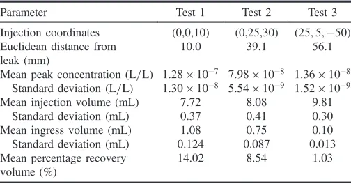
(25;5;−50) respectively. Table 2 summarizes the results from the three detailed example tests presented, showing the mean values from the five repeat tests for each discrete injection location.

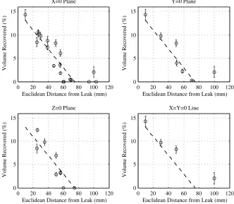
A total of 61 different point source locations distributed around the leak were studied. The mean recovery volumes for each discrete location were calculated and plotted against the Euclidean distance as shown in Fig.8. A linear trend line (dashed line) was fitted to the data, defined by the equationVð%Þ ¼15.03−0.20ðDÞproducing anR2of 0.774, whereVis the percentage volume of dye recovered andDis the Euclidean distance from the leak (mm). All data points with zero recovered volume were removed during the regression analysis in order to determine a threshold value for zero ingress, using the developed trend line. The compiled results shown in Fig.8 illustrate that the magnitude of contaminant ingress decreases with increasing distance from the leak orifice. Fig.9shows the standard deviation associated with the recorded data for the repeat tests in three main reference planes, wherex¼0,y¼0, andz¼0, and a single line above the leak orifice, wherex¼y¼0, alongside the linear trend line defined in Fig.8.

Discussion

The qualitative experimental results provide good proof of the net intrusion of external contaminant into a pressurized pipe due to 0 20 40 60 80 100 120

0 0.5 1 1.5x 10

−7

Time (s)

Concentration (l/l)

Intrusion Level Fluorometer Background Level Fluorometer

0 20 40 60 80 100 120 −20

−10 0 10 20 30

Time (s)

Pressure Head (m)

Pollutant Injection Start and Stop Time

Fig. 5. Representative point source pollutant injection location at (0,0,10); background and intrusion fluorometer traces and synchronous pressure head at test section

0 20 40 60 80 100 120 0

0.5 1 1.5x 10

−7

Time (s)

Concentration (l/l)

Intrusion Level Fluorometer Background Level Fluorometer

0 20 40 60 80 100 120 −20

−10 0 10 20 30

Time (s)

Pressure Head (m)

Pollutant Injection Start and Stop Time

Fig. 6. Representative point source pollutant injection location at (0,25,30); background and intrusion fluorometer traces and synchro-nous pressure head at test section

0 20 40 60 80 100 120 0

0.5 1 1.5x 10

−7

Time (s)

Concentration (l/l)

Intrusion Level Fluorometer Background Level Fluorometer

0 20 40 60 80 100 120 −20

−10 0 10 20 30

Time (s)

Pressure Head (m)

Pollutant Injection Start and Stop Time

Fig. 7. Representative point source pollutant injection location at (25;5;−50); background and intrusion fluorometer traces and synchro-nous pressure head at test section

Table 2. Experimental Results for Three Discrete Injection Locations: Mean Values from the Five Repeat Tests for Each Location Are Summarized

Parameter Test 1 Test 2 Test 3

Injection coordinates (0,0,10) (0,25,30) (25;5;−50)

Euclidean distance from leak (mm)

10.0 39.1 56.1

Mean peak concentration (L=L) 1.28×10−7 7.98×10−8 1.36×10−8

Standard deviation (L=L) 1.30×10−8 5.54×10−9 1.52×10−9

Mean injection volume (mL) 7.72 8.08 9.81

Standard deviation (mL) 0.37 0.41 0.30

Mean ingress volume (mL) 1.08 0.75 0.10

Standard deviation (mL) 0.124 0.087 0.013

Mean percentage recovery volume (%)

14.02 8.54 1.03

negative transient pressures. The work showed that no re-extrusion of the contaminant occurred and even for a leak into water only, not all the contaminant was washed away or diluted by the leak flow during the initial steady-state conditions prior to the initiation of the transient. Such visual evidence is useful for informing operational staff of the risk of contaminant ingress into water distribution systems.

The quantitative experimental methodology and test procedure developed to explore the phenomena of contaminant ingress during a transient event was shown to be very repeatable and produced consistent data. This is highlighted by the repeatability of the gen-erated transients shown in Fig.3and the relatively low variability

between repeat tests displayed by the error bars shown in Fig.9. Data presented in Fig.8 shows a negative linear association be-tween the Euclidean distance of the pollutant injection from the leak and the volume of pollutant measured downstream of the leak point. This inverse relationship between the distance of a point source pollutant to a leak and the volume of ingress determined under physically representative conditions corresponds with the concept of a zone of influence surrounding a leak as presented by Collins et al. (2011b). This zone of influence indicates the flow path lines into the leak from different regions, and therefore distan-ces, in an external porous media, providing a means to conceptu-alize the risk of contaminant ingress considering the location of the pollutant external to a leak. It is significant that volume is primarily a function of distance and not location relative to the pipe, as this counters the practitioner argument that the risk is primarily from sources above the pipe; i.e., not leaking sewers which are usually below distribution pipes. The results presented here confirm that there is a real risk of contaminant ingress from all pollutant sources located within the three-dimensional zone of influence, where a bigger negative transient will result in a larger zone of influence. The quantifiable risk of contaminant ingress is therefore a function of scale of the zone of influence and the distance of the point source pollutant from the leak.

Although not investigated in detail here, the magnitude of contaminant ingress may also be influenced by several additional factors. These include the size and duration of the pressure tran-sient, dependent on the initial flow and pressure conditions and the characteristics of the system, as well as the size of the leak which has complicated energy dissipation effects impacting the dis-sipation of the generated pressure waves. Further, the nature of the media external to the pipe will influence the energy dissipation, flow rates, and zone of influence. First approximations of these

0 20 40 60 80 100 120

0 2 4 6 8 10 12 14 16

Euclidean Distance from Leak (mm)

Percentage Volume Recovered (%)

Mean Recovered Volume Linear Trend Line

Fig. 8.Relationship between the discrete point source pollutant Eucli-dean distance from the leak, and the percentage volume of injected dye recovered, including associated1standard deviation error bars

0 20 40 60 80 100 120

0 5 10 15

Euclidean Distance from Leak (mm)

Volume Recovered (%)

X=0 Plane

0 20 40 60 80 100 120

0 5 10 15

Euclidean Distance from Leak (mm)

Volume Recovered (%)

Y=0 Plane

0 20 40 60 80 100 120

0 5 10 15

Euclidean Distance from Leak (mm)

Volume Recovered (%)

Z=0 Plane

0 20 40 60 80 100 120

0 5 10 15

Euclidean Distance from Leak (mm)

Volume Recovered (%)

X=Y=0 Line

Fig. 9.Data from the three main reference planes (wherex¼0,y¼0, and z¼0) and single line above the leak (wherex¼y¼0) including associated standard deviation error bars, plotted against linear trend line for the whole data set (dashed line) evaluated in Fig.8

may be gained from the steady-state work presented in Collins and Boxall (2013).

For each repeat, three pressure transients were generated, the first during the injection of the pollutant. The downstream fluorom-eter only recorded one pulse of pollutant at a time consistent with the travel time in the pipe. The results indicate that, in the test cases, flows from the leak were able to dilute and flush the pollutant away from the ingress area before the second and third transients were generated. This effect was also evident within the qualitative test conducted, Fig.4. However, this does not necessarily mean that all pollutants would be automatically flushed away in a real system. The effect of groundwater flows may serve to renew pollutant in to the zone of ingress, or small particulate contaminate may be trapped within the zone. Additionally, the dynamics of a leak jet into water or fluidized soil potentially creates recirculating vortices surrounding the leak orifice (van Zyl et al. 2013). Such recircula-tion due to a leak jet could therefore also draw contaminant in to the zone of ingress. Further work is required to fully understand the zone of influence for ingress, the effects of groundwater flows and soil mechanics in presenting contaminants into the ingress zone. The presented work consists of a single finite magnitude point source pollutant; although in reality we may also expect the existence of an unlimited pollutant source around the leak, non-uniformly distributed within the surrounding media such as due to net ground water flow bringing a contaminant plume from a leaking sewer.

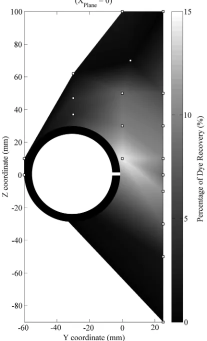
In order to understand the zone of influence from which pollu-tants may be drawn through a leak into a WDS pipe, a wide range of discrete point source locations within a three-dimensional space surrounding the pipe were investigated within the experimental work. Fig.10 highlights the importance of considering the zone of influence, where contaminants located in all directions from a single leak may be susceptible to the effects of negative pressure transients within the pipe, resulting in contaminant ingress. An anecdotal impression that only those contaminants located above the leak or along the line of thejetfrom the leak are susceptible to the phenomena of ingress as introduced by the authors is negated by the recorded data which showed significant ingress of the representative point source pollutant from below the axis of the leak. This was also shown for locations adjacent to the leak, above and below the origin. This phenomenon is due to dissipation effects of the surrounding media as highlighted in Collins et al. (2011b). The ovality of the contaminant ingress contours depicted in Fig.10, biased above the horizontally orientated leak orifice, reflect the composition of the zone of influence developed by Collins et al. (2011b) using a steady-state computational fluid dynamic (CFD) model. These models defined the flow path lines surrounding an orifice during a steady-state intrusion event. By referencing these models it can be reasoned that the Euclidean distance used within the aforementioned experimental work is not directly equivalent to the flow path line distance that the point source pollutant travels along when drawn into the pipe. It may be inferred that the shorter the flow path line distance to the leak from the point source pollu-tant, the greater the resulting volume of contaminant ingress. In the CFD simulations the flow path line length for discrete locations with equal Euclidean distance was shorter for those flow path lines directly above the vertically orientated leak compared with those in other directions. Similarly, these physical experimental results, shown in Fig.9for the injection locationsx¼y¼0, i.e., directly above the leak, display the highest volumes of pseudo pollutant ingress, a phenomenon that may be interpreted as a direct result of the formation of preferential flow lines for the leakage flow to the gravel surface. However, this interpretation is potentially lim-ited due to the steady-state conditions used within the CFD model

as opposed to the transient conditions used within the experimental investigation, the difference between the orientation of the leak or-ifices in the two situations and also potential uncertainty in absolute intrusion volumes based on the linear interpolation conducted between the discrete injection locations in Fig.10.

Modeling-based research has attempted to identify and quantify the risks of contaminant ingress across different networks (Sadiq et al. 2006;Deng et al. 2011;Ebacher et al. 2012). These typically include estimation of intrusion volume using the orifice equation. However the work presented here suggests that this is likely to overestimate the volume of pollutant ingress. The orifice equation will provide a worst case, upper bound, estimate of the maximum volume of fluid intruded, not the pollutant volume specifically. The equation misses the resistance effects of ground conditions, reducing the volume, as highlighted for steady-state conditions by Collins and Boxall (2013). It also does not represent the zone of influence effects reported here and the low recovery percentages observed here. Thus, the work presented suggests that the risk of direct exposure (the threat to human health due to consumption of water directly contaminated by intrusion) is significantly less than estimated by previous modeling studies. Further the risk due to the overestimated volumes reported by these modeling stud-ies may be further reduced by consideration of reaction with dis-infection residuals. However, this does not consider the risk of Fig. 10.Contour plot, using linear interpolation, showing experimental results of the dye recovery percentage in single plane (x¼0) external to 5 mm engineered leak orifice; discrete injection locations indicated by small squares

indirect exposure, such as the seeding of pathogenic organisms into biofilms. In this scenario even very small volumes of contaminant can seed a biofilm local to the site of ingress with pathogenic organisms, that can then be protected from the disinfection residual within the bulk water and potentially survive and proliferate within the biofilm and further seed the downstream system. At some point in the future the biofilm may lose strength or be disturbed, such as due to hydraulic changes in the system, and biofilm containing pathogens originating from the intrusion event may be mobilized with a variety of other material that rapidly depletes the disinfection residual and hence does pose a risk to human health. Discoloration research has confirmed the association between biofilm hydraulic mobilization and organic and inorganic material in water quality samples (Douterelo et al. 2014). Disinfection depletion has also been observed in these samples. Further research is required to better understand the behavior of pathogenic organisms within biofilms, in particular the impact of different bulk water character-istics such as organic carbon and disinfection strategy on biofilm communities and matrix, and the ability for pathogens to shelter and proliferate within them.

Conclusions

The results of the novel experimental work reported here showed that under extreme, but realistic, conditions the ingress of contam-inants originating externally to a leak orifice in a pressurized pipe can occur due to the occurrence of pressure transients within the system. The perception that only water expelled from the pipe, under positive steady-state or dynamic pressures, will reenter through the leak has been shown to be unfounded as has the re-extrusion of contaminant on the next positive cycle of the transient. Contaminants have been shown to be ingressed from a significant area outside the leak, with the ingress volume having an inverse relationship with the distance of the contaminant from the leak. Three detailed example results for different representative point sources of pollutant are presented, with increasing Euclidean dis-tance from the leak, demonstrating that contaminants can be drawn into the pipe from a significant area outside the orifice. Results of 61 different injection locations are also summarized showing the ingress volume having an inverse relationship with the distance of the contaminant from the leak, but largely independent of loca-tion (e.g., above, below).

This paper conclusively shows, for the first time, that for fully representative physical conditions, there is a threat to potable water quality due to net contaminant ingress and transport during extreme short duration oscillating pressure transient events within water distribution networks.

Acknowledgments

The research reported in this paper was supported by EPSRC grant EP/G015546/1 and EPSRC platform grant EP/I029346/1.

References

Boyd, G., et al. (2004).“Intrusion within a simulated water distribution

system due to hydraulic transients. I: Description of test rig and

chemi-cal tracer method.”J. Environ. Eng.,10.1061/(ASCE)0733-9372(2004)

130:7(774), 774–777.

Brunone, B., and Ferrante, M. (2004).“Pressure waves as a tool for leak

detection in closed conduits.”Urban Water J., 1(2), 145–155.

BSI (British Standards Institution). (1973).“Code of practice for plastics

pipework (thermoplastics material). Part 1: General principles and

choice of material.”CP 312-1:1973.

Clayton, C., and van Zyl, J. (2007).“The effect of pressure on leakage

in water distribution systems.” Proc. ICE Water Manage., 160(2),

109–114.

Collins, R., Beck, S., and Boxall, J. (2011a). “Intrusion into water

distribution systems through leaks and orifices: Initial experimental

re-sults.”Proc., 11th Computing and Control in the Water Industry, Centre

for Water Systems, Univ. of Exeter, U.K.

Collins, R., and Boxall, J. (2013). “Influence of ground conditions on

intrusion flows through apertures in distribution pipes.”J. Hydraul.

Eng.,10.1061/(ASCE)HY.1943-7900.0000719, 1052–1061.

Collins, R., Boxall, J., Besner, M. C., Beck, S., and Karney, B. (2011b).

“Intrusion modelling and the effect of ground water conditions.”

Proc., Water Distribution Systems Analysis 2010, ASCE, Reston, VA,

585–594.

Collins, R., Boxall, J., Karney, B., Brunone, B., and Meniconi, S. (2012a).

“How severe can transients be after a sudden depressurization?”

Am. Water Works Assoc., 104(4), E243–E251.

Collins, R., Fox, S., Beck, S., Saul, A., and Boxall, J. (2012b).“Intrusion

and leakage through cracks and slits in plastic (MDPE) pipes.”

Proc., 14th Water Distribution Systems Analysis Conf., Engineers Australia, Barton, ACT, Australia.

Deng, Y., Jiang, W., and Sadiq, R. (2011). “Modeling contaminant

intrusion in water distribution networks: A new similarity-based

DST method.”Expert Syst. Appl., 38(1), 571–578.

Douterelo, I., Husband, S., and Boxall, J. B. (2014).“The bacteriological

composition of biomass recovered by flushing an operational drinking

water distribution system.”Water Res., 54, 100–114.

Ebacher, G., Besner, M. C., Clément, B., and Prévost, M. (2012).

“Sensitivity analysis of some critical factors affecting simulated

intrusion volumes during a low pressure transient event in a full-scale

water distribution system.”Water Res., 46(13), 4017–4030.

Eboigbodin, K., Seth, A., and Biggs, C. (2008).“A review of biofilms

in domestic plumbing.” J. Am. Water Works Assoc., 100(10),

131–138.

Fox, S., Collins, R., and Boxall, J. (2012).“Time dependent area of leaks in

MDPE pipes during transient events.”Proc., 11th Int. Conf. on Pressure

Surges, BHR Group, Bedford, U.K., 113–125.

Fox, S., Shepherd, W., Collins, R., and Boxall, J. (2013).“Experimental

proof of contaminant ingress into a leaking pipe during a transient

event.” Proc., 12th Computing and Control in the Water Industry,

Elsevier, Amsterdam, Netherlands.

Ghidaoui, M., Zhao, M., McInnis, D., and Axworthy, D. (2005).“A review

of water hammer theory and practice.”Appl. Mech. Rev., 58(1),

49–76.

Gullick, R., Lechevallier, M., Svindland, R., and Friedman, M. (2004).

“Occurrence of transient low and negative pressures in distribution

systems.”J. Am. Water Works Assoc., 96(11), 52–66.

Hunter, P., Chalmers, R., Hughes, S., and Syed, Q. (2005).“Self-reported

diarrhea in a control group: a strong association with reporting of

low-pressure events in tap water.”Clin. Infect. Dis. Off. Publ. Infect.

Dis. Soc. Am., 40(4), e32–e34.

Karim, M., Abbaszadegan, M., and Lechevallier, M. (2003). “Potential

for pathogen intrusion during pressure transients.”J. Am. Water Works

Assoc., 95(5), 134–146.

Kirmeyer, G., et al. (2001). Pathogen intrusion into the distribution

system, AWWA Research Foundation and the American Water Works Association, Denver.

Lechevallier, M., Gullick, R., Karim, M., Friedman, M., and Funk, J.

(2003).“The potential for health risks from intrusion of contaminants

into the distribution system from pressure transients.”J. Water Health,

1(1), 3–14.

Lindley, T., and Buchberger, S. (2002).“Assessing intrusion susceptibility

in distribution systems.”J. Am. Water Works Assoc., 94(6), 66–79.

L´opez-Jiménez, P., and Mora-Rodríguez, J. (2010). “3D computational

model of external intrusion in a pipe across defects.”Proc., Int.

Envi-ronmental Modelling and Software Society (iEMSs) 2010 Int. Congress on Environmental Modelling and Software Modelling for Environments

Sake, International Congress on Environmental Modelling and Soft-ware, San Diego.

Mora-Rodríguez, J., L´opez-Jiménez, P., and Ramos, H. (2011).“Intrusion

problematic during water supply systems’ operation.”Int. J. Energy

Environ., 2(3), 391–400.

Ofwat. (2010).“Service and delivery performance of the water companies

in England and Wales 2009-10 report supporting information.”〈http://

www.ofwat.gov.uk/regulating/reporting/rpt_los_2009-10supinfo.pdf〉

(Jul. 5, 2013).

Sadiq, R., Kleiner, Y., and Rajani, B. (2006). “Estimating risk of

contaminant intrusion in water distribution networks using

Dempster Shafer theory of evidence.” Civ. Eng. Environ. Syst.,

23(3), 129–141.

Starczewska, D., Collins, R., and Boxall, J. (2013).“Transient behavior in

complex distribution network: A case study.”Proc., 12th Computing

and Control in the Water Industry, Elsevier, Amsterdam, Netherlands. van Zyl, J., Alsaydalani, M., Clayton, C., Bird, T., and Dennis, A. (2013).

“Soil fluidisation outside leaks in water distribution pipes preliminary

observations.”Water Manage., 166(WM10), 546–555.

van Zyl, J., and Cassa, A. (2014).“Modeling elastically deforming leaks in

water distribution pipes.”J. Hydraul. Eng.,10.1061/(ASCE)HY.1943

-7900.0000813, 182–189.