Omni-conducting and omni-insulating molecules
P. W. Fowler,1,a)B. T. Pickup,1,b) T. Z. Todorova,1,c)Martha Borg,1,d)and Irene Sciriha2,e)
1Department of Chemistry, The University of Sheffield, Sheffield S3 7HF, United Kingdom 2Department of Mathematics, Faculty of Science, University of Malta, Msida MSD 2080, Malta
(Received 21 November 2013; accepted 16 January 2014; published online 6 February 2014)
The source and sink potential model is used to predict the existence of conductors (and omni-insulators): molecular conjugatedπ systems that respectively support ballistic conduction or show insulation at the Fermi level, irrespective of the centres chosen as connections.Distinct,ipso,and strongomni-conductors/omni-insulators show Fermi-level conduction/insulation for alldistinctpairs of connections, for all connections via asinglecentre, and forboth, respectively. The class of con-duction behaviour depends critically on the number of non-bonding orbitals (NBO) of the molecu-lar system (corresponding to the nullity of the graph). Distinct omni-conductors have at most one NBO; distinct omni-insulators have at least two NBO; strong omni-insulators do not exist for any number of NBO. Distinct omni-conductors with a single NBO are all also strong and correspond exactly to the class of graphs known asnutgraphs. Families of conjugated hydrocarbons correspond-ing to chemical graphs with predicted omni-conductcorrespond-ing/insulatcorrespond-ing behaviour are identified. For ex-ample, most fullerenes are predicted to be strong omni-conductors. © 2014 AIP Publishing LLC. [http://dx.doi.org/10.1063/1.4863559]
I. INTRODUCTION
Ballistic conduction on nano and mesoscopic scales is at-tracting ever increasing interest with the availability of new materials such as graphene sheets and flakes1(potentially in kilogram amounts2). One starting point for theoretical ac-counts of this type of conduction is the study of molecular conjugated structures, where electron transmission is known to be a sensitive function of, amongst others, three major fac-tors, namely, electron energy, contact position, and underlying molecular structure. The field has a long history, and methods continue to be developed.3 Sophisticated ab initio methods
for obtaining detailed information on molecular conduction in particular systems have been developed (e.g., Refs.4–9). An alternative approach,10–13 which we take here, is to use
qualitative models to focus on generic types of conduction behaviour.
A simple approach which is capable of dealing with π systems is the graph theoretical source and sink potential (SSP) model.13–22 The present work is concerned with this model and the information that it may give about the interac-tion of the factors of contact posiinterac-tion and molecular structure. In particular, we explore the possibility that some molecu-lar structures may display a much reduced dependence of the predicted transmission on precise positioning of the contacts. Given the difficulties of attaching “wires” with atomic resolu-tion, such insensitivity may have some practical advantages. This motivates our definitions ofomni-conductorsand omni-insulatorsand the search for classes of chemical graphs that conform to these definitions.
a)Electronic mail: P.W.Fowler@sheffield.ac.uk b)Electronic mail: B.T.Pickup@sheffield.ac.uk c)Electronic mail: chp07tzt@sheffield.ac.uk d)Electronic mail: mborg1@sheffield.ac.uk e)Electronic mail: irene.sciriha-aquilina@um.edu.mt
A molecule will be modelled by itsmolecular graph G, which represents the carbon skeleton of a conjugatedπ sys-tem.Chemical graphsare defined as graphs that are connected and have maximum degree at most three; their vertices repre-sent unsaturated carbon centres and their edges reprerepre-sent the σ-bond framework. If we set aside the dependence of trans-mission on energy by considering conduction to take place at the Fermi level (corresponding to the zero of energy in the Hückel/SSP model) and consider the molecule to be con-nected to similar left and right wires via its atoms ¯Land ¯R, a natural question arises: Do conjugated molecular structures exist for which there is conduction (non-zero transmission) at the Fermi level forallchoices of connections ¯Land ¯R? An equivalent question can be asked about insulation (zero trans-mission).
We can imagine two types of connection of the wires to “terminal” vertices ¯L and ¯R in the molecular graph: either the connecting vertices aredistinct, which is the relevant case for most applications, or they coincide, which is the so-called “ipso” case. The fractional transmission of a ballistic electron at the Fermi level for a given connection pair ( ¯L, ¯R), which is here calculated within the SSP model, will be denotedT(0). The combination of a graphGand a pair of contact vertices, not necessarily distinct, will be called here adevice. Hence, from this point of view, there are in principle six interesting classes of molecular graphs and the devices related to them.
1. A molecular graph is said to be a distinct omni-conductorifT(0)=0 foralldistinct pairs of connecting vertices, ¯Land ¯R.
2. A molecular graph is said to be anipso omni-conductor ifT(0)=0 forallchoices of single-vertex connection,
¯ L=R¯.
3. A molecular graph is said to be astrong omni-conductor if it is both adistinctand anipsoomni-conductor.
4. A molecular graph is said to be adistinct omni-insulator ifT(0) =0 foralldistinct pairs of connecting vertices (terminals), ¯Land ¯R.
5. A molecular graph is said to be anipso omni-insulator ifT(0)=0 forallchoices of single-vertex connection,
¯ L=R¯.
6. A molecular graph is said to be astrong omni-insulator if it is both adistinctand anipsoomni-insulator.
In fact, the sixth class turns out to be empty, as we will prove, but all other classes include molecular graphs of chem-ical interest.
A molecule with non-bonding orbitals corresponds to a singular graph, and the number of non-bonding orbitals is equal to the nullity: the number of zero eigenvalues of the adjacency matrix of the graph. It has already been shown that the numbers of non-bonding levels of molecular graphs and subgraphs are important in defining selection rules for Fermi-level conduction of given connection pairs in general,18 and for graphene-related molecular graphs in particular.19 Here,
it will be demonstrated that nullity is also a crucial factor in characterising omni-conductors and omni-insulators. Specif-ically, we will prove that alldistinct omni-conductors have at most one non-bonding orbital whereas alldistinct omni-insulators have at least two, and will give a complete charac-terisation of the nullity-one distinct omni-conductors.
The paper is arranged as follows. After a brief summary of the SSP model and graph theoretical background (Sec.II), we give a unified treatment of the selection rules for Fermi-level conduction/insulation of individual devices in terms of characteristic polynomials, nullity of graphs, and vertex types (Secs.IIIandIV). This leads to existence and characterisation results for the six classes of omni-conductors and insulators (Sec. V). In Sec. VI, explicit calculations for large numbers of graphs in various chemically interesting classes and infinite families are presented, with statistical information about the distribution of the different classes, leading to the conclusion (Sec.VII) that omni-conduction at the Fermi level could be a widely occurring phenomenon.
II. BACKGROUND
A. The SSP model
The SSP Hamiltonian gives a simple model of ballistic conduction of electrons through a conjugated molecule.12,14,15In the tight-binding approximation,
calcula-tion of the fraccalcula-tional transmission of an electron with given energy reduces to the solution of the Hückel problem un-der scattering boundary conditions, and hence to an es-sentially graph theoretical question, as conduction is deter-mined by functions of the characteristic polynomials of four graphs.13,16–19
In the SSP model, the transmission function for a molecule that has a carbon skeleton with graphGconnected to similar left and right wires via molecular vertices ¯Land ¯R is given by13
T (E)= 4 sin
2q(ut−sv) ˜β2
|e−2iqs−e−iq(u+t) ˜β+vβ˜2|2, (1)
where E is the reduced electron energy, defined on a scale where the unit is the molecular resonance integral |β|, and the zero is the molecular coulomb integralα, which is taken here as the Fermi level. Coulomb integrals are assumed to be equal throughout the device, and the parameter ˜β is defined by the values of resonance integrals within wires (βL =βR)
and between molecule and wire (βLL¯ =βRR¯), in units of the
molecular resonance integral β (which is the unit for all en-ergies occurring in the model): ˜β=βL2L¯/βL=βR2R¯/βR. Typ-ically, ˜β21/2.13,14 The 4 sin2q factor in (1) acts to con-fine transmission to the conduction band of the wires. In(1) q is the wavenumber of the electron wave (defined by E = 2cosq, with energy in units of |β|). The
quanti-ties s, t, u, v are the characteristic polynomials φ(G, E),
φ(G−L, E¯ ),φ(G−R, E¯ ),φ(G−L¯−R, E¯ ) of the graphs G,G−L¯,G−R¯, andG−L¯−R¯, respectively, i.e., they are the determinants
s(E) = |EI−A(G)|,
t(E) = |EI−A(G−L¯)| = |EI−A(G)|L,¯L¯,
(2) u(E) = |EI−A(G−R¯)| = |EI−A(G)|R,¯R¯,
v(E) = |EI−A(G−L¯ −R¯)| = |EI−A(G)|L¯R,¯L¯R¯,
where Iis the identity matrix of the appropriate dimension and A(H) is the adjacency matrix of a graphH. Note that G must be a connected graph if it is to represent a conju-gated π system; deletion of vertices as in G−L¯, G−R¯, andG−L¯−R¯ may result in a disconnected graph. The su-perscripts on the determinants indicate deletion of a set of rows and columns, corresponding to the deletion of vertices ofG. Another quantity that is important in the determination of transmission is the combinationut −sv, which is equal to a squared polynomial23
j2(E)=u(E)t(E)−s(E)v(E)=(|EI−A(G)|L,¯R¯)2. (3)
It can be shown thatj(E) is the entry at position ¯L,R¯ of the adjugate matrix adj(EI−A) and, if the matrix (EI−A) is invertible, then at any energy E, j(E) is proportional to the
¯
L,R¯entry in the inverse (EI−A)−1, with constant of
propor-tionality equal to the determinant of the matrix.24 The usual
distinct case for a molecular device has ¯L=R¯. In the ipso case, where both wires contact a single atom, ¯L=R¯, polyno-mialstanduare identical, andvis deleted from the equations. AsE=2cosq, the full energy dependence of the trans-mission(1)is given by
T(E)= (4−E
2)j2β˜2
and for transmission of electrons at the Fermi level, the limit is taken according to
T(0)= lim
E→0T(E).
In the analysis that follows, we assume that ˜β2is not a
“spe-cial value,” i.e., we assume that ˜β =0 and that (s−vβ˜2)2
=0 at the energy of interest. Thus, effectively, questions about the vanishing of (s−vβ˜2)2can be answered by
inspec-tion of s2+v2. Physically, the claim is that even if ˜β
hap-pens to take one of the special values, there will always be a “nearby” device where it does not, and to which our generic conclusions will apply.
It is straightforward to show that the zero-energy limit of (4)is equivalent to the simpler expression
T(0)= lim
E→0
4j2β˜2
[(s−vβ˜2)2+(u+t)2β˜2]. (5)
The question for a qualitative treatment is whetherT(0) is zero, or not. It has been shown18that the answer to this
ques-tion for a given connecques-tion pattern can be decided in almost all cases simply by counting the zero eigenvalues of the graph and of its vertex-deleted subgraphs, which leads to a set of “selection-rules” for conduction. In order to exploit this in-sight further, and make a systematic investigation of the ques-tions of omni-conduction and insulation, it is necessary to un-derstand how the outcome depends on the intrinsic properties of the connecting vertices relative to the nullspace vectors. To help with this task, we introduce some notation and results from graph theory and linear algebra in Sec.II B. More detail on the mathematical arguments can be found in Ref.25.
B. Graph theoretical notation
The eigenvalue problem for the adjacency matrixAof a graph is
Aci =Eici, (6)
where for some non-zero vector cithe matrix has an
eigen-value Ei. For a n-vertex graph G, the n values of Ei form
thespectrumofG. The eigenvectorsciofAcorrespond toπ
molecular orbitals in the Hückel approximation and without loss of generality the entriescir can be taken to be real. (Here the subscript rdenotes the vertex and the superscript i the molecular orbital.) For conduction of a connectedπ-systemG at the Fermi level, (E=0), it is critical to consider the number of non-bonding orbitals. This number is the multiplicitygsof
the zero eigenvalue in the spectrum, also called thenullityof the graph. A graph is singularifgs >0. We shall organise
the eigenvectors ci of the adjacency matrix such that theg s
eigenvectors in the nullspace are placed first.
A vector cin the nullspace of the adjacency matrix A is said to be akernel eigenvector of G. For singular graphs the vertices can be partitioned intocore andcore-forbidden vertices. Acore-forbidden vertex(CFV) corresponds to a zero entry ineverykernel eigenvector. A vertex corresponding to a non-zero entry forsomekernel eigenvector is acore vertex (CV). Core graphs are defined as singular graphs in which each vertex is a core vertex. A core graph of nullity one is
termed anut graph. Nut graphs are connected, non-bipartite and have no vertices of degree one.26
The Interlacing Theorem27 states that the eigenvalues
of a vertex-deleted subgraph interlace the eigenvalues of the parent graph. As a consequence, the multiplicity (num-ber of repetitions) of any one eigenvalue in the spectrum changes by at most one on deletion of a vertex. A nec-essary and sufficient condition for the nullity to decrease on deletion of a vertex from a graph is that the deleted vertex is a CV. Therefore, by interlacing, deletion of a CFV either leaves the nullity unchanged or increases it by one. We call a CFV upper where the nullity increases and middlewhere the nullity remains unchanged. In this language, a CV is said to belower. Other terms are also used in the lit-erature: the CFVs are referred to as peripheral vertices; up-per vertices are variously termed maximal,28 Parter, or
rank-strong vertices;29 middle vertices are called intermediate28
or rank-neutral;29 and lower vertices are also called downer
or rank-weak vertices.29 Bipartite graphs do not have middle vertices.
C. Characteristic polynomials
For a graphGof nullitygs, the characteristic polynomial
is
s(E)= n
i=1
(E−Ei)=s0(E)Egs, (7)
wheres0(E) is the product over the non-nullspace
s0(E)= n
i=gs+1
(E−Ei). (8)
Note thats0(0)=0. We will writes0fors0(E),sfors(E), etc.,
where there is no ambiguity.
The other polynomialst(E),u(E),j(E), andv(E) can be expressed in terms of the eigenvector entries {cLi¯}and{ciR¯} associated with the connecting vertices ¯Land ¯R, as described in Ref.25. (As noted earlier, we are assuming that all eigen-vector entries are real.) These polynomials are
t(E)= n
i=1
ciL¯2 j=i
(E−Ej)= n
i=1
cLi¯2
E−Eis0(E)E gs,
(9)
u(E)= n
i=1
ciR¯2 j=i
(E−Ej)= n
i=1
ci
¯
R
2
E−Eis0(E)E gs,
(10)
j(E)= n
i=1
ciL¯ciR¯ j=i
(E−Ej)= n
i=1
ci
¯
Lc i
¯
R
E−Ei
s0(E)Egs.
(11) Since the first gs eigenvectors belong to the nullspace,
explicit dependence onE:
t(E)= gs
i=1
cLi¯2s0(E)Egs−1+
n
i=gs+1
ci
¯
L
2
E−Eis0(E)E gs
=tbEgs−1+taEgs, (12)
u(E)= gs
i=1
ciR¯2s0(E)Egs−1+
n
i=gs+1
ciR¯2
E−Eis0(E)E gs
=ubEgs−1+uaEgs, (13)
j(E)= gs
i=1
ciL¯ciR¯s0(E)Egs−1+
n
i=gs+1
ciL¯ciR¯
E−Ei
s0(E)Egs
=jbEgs−1+jaEgs. (14)
Hence, using (3), the characteristic polynomial for the two-vertex deleted graph,v(E), splits into three:
v(E)=vcEgs−2+vbEgs−1+vaEgs, (15)
where
va = 1
s0
uata−ja2=1 2s0
n
i=gs+1
n
j=gs+1
ciL¯cjR¯ −cjL¯ciR¯2
(E−Ei)(E−Ej), (16)
vb=1
s0
(uatb+ubta−2jajb)=s0
gs
i=1
n
j=gs+1 ci ¯ Lc j ¯
R−c j ¯ Lc j ¯ R 2
E−Ej
,
(17)
vc= 1 s0
ubtb−jb2
= 1
2s0 gs
i=1
gs
j=1
cLi¯cjR¯ −cLj¯ciR¯2, (18)
and in particular
ja2=uata−s0va, (19)
jajb= 1
2(uatb+ubta−s0vb), (20)
jb2=ubtb−s0vc, (21)
so thatva,vb, andvccan be derived directly from the seven quantities s0, ta, . . . jb. All the above expressions apply to
cases withgs ≥2. Forgs =1, the term invc is to be set to
zero, and, forgs =0, only the terms inta,ua,ja, andva are
present.
An expression for T(E) can now be assembled, and its limit taken using the numerator and denominator terms from (5). The numerator is
4 ˜β2j2=4 ˜β2ja2E2+2jajbE+jb2
[image:4.612.62.302.63.272.2]
E2gs−2, (22)
TABLE I. The seven conditions for insulation.
gs=0 ja=0
gs=1
⎧ ⎪ ⎪ ⎪ ⎪ ⎪ ⎪ ⎪ ⎨ ⎪ ⎪ ⎪ ⎪ ⎪ ⎪ ⎪ ⎩
jb=0 andja=0
or
jb=0 andja=0
⎧ ⎪ ⎪ ⎨ ⎪ ⎪ ⎩
ub+tb=0
or
vb=0
,
gs>1
⎧ ⎪ ⎪ ⎪ ⎪ ⎪ ⎪ ⎪ ⎨ ⎪ ⎪ ⎪ ⎪ ⎪ ⎪ ⎪ ⎩
vc=0
or
vc=0
⎧ ⎪ ⎪ ⎨ ⎪ ⎪ ⎩
jb=0 andja=0 andvb=0 andub+tb=0
or
jb=0 andja=0
.
and the denominator is
(s−β˜2v)2+(u+t)2β˜2
=E4[(s0−β˜2va)2+(ua+ta)2β˜2]
+E3[−2vb(s0−vaβ˜2) ˜β2+2(ua+ta)(ub+tb) ˜β2]
+E2vb2−2vc(s0−vaβ˜2)+(ub+tb)2
˜ β2
+E[2vbvc] ˜β4+vc2β˜4E2gs−4. (23)
As both numerator and denominator may vanish at E =0, it is not sufficient simply to examine whetherj van-ishes to determine the conduction or insulation behaviour of a device with a given pair of contacts. In general, it is necessary to delve more deeply into the cancellation behaviour of the numerator and denominator asEapproaches zero.
[image:4.612.53.299.320.626.2]The advantage of the present formulation forT(E) is that the conductive properties of all devices based on a given molecular graph can be determined from a simple calcula-tion of the eigenvectors and eigenvalues ofGalone. No sepa-rate calculations on thenvertex-deleted graphsG−wor the n(n −1)/2 double-deleted graphs G−w−z are required. This gives the basis for an efficient computational scheme for identifying omni-conductors and omni-insulators. Conditions for insulation or conduction for a distinct pair of contact ver-tices in a graph with a particular nullity are easily deduced (TablesIandII); analogous conditions for ipso connections are derived by settingva=vb=vc=0,ua=ta, andub=tb.
TABLE II. The seven conditions for conduction.
gs=0 ja=0
gs=1
⎧ ⎪ ⎪ ⎪ ⎪ ⎪ ⎪ ⎨ ⎪ ⎪ ⎪ ⎪ ⎪ ⎪ ⎩
jb=0
⎧ ⎪ ⎪ ⎨ ⎪ ⎪ ⎩
ub+tb=0
or
vb=0
or
jb=0 andja=0 andub+tb=0 andvb=0,
gs>1
⎧ ⎪ ⎪ ⎪ ⎪ ⎪ ⎪ ⎨ ⎪ ⎪ ⎪ ⎪ ⎪ ⎪ ⎩
vc=0 andjb=0
⎧ ⎪ ⎪ ⎨ ⎪ ⎪ ⎩
ub+tb=0
or
vb=0
or
The reader interested only in the results could now skip to Sec.V, where the global deductions about classes of con-ductors are summarised, and then to Sec.VIwhere results for specific families of chemical graphs are described.
III. DEVICES AND VARIETIES
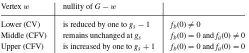
The various contributionsuatovchave different limiting behaviour, depending on the types of the contact vertices. In particular, if the characteristic polynomial of a vertex-deleted subgraphG−wof a graphG(withwa generic vertex) is cast in the form
φ(G−w, E)=fb(E)Egs−1+fa(E)Egs, (24)
then the values offaandfbatE=0 distinguish the three types
of vertex and their effect on the nullity as follows:
Vertexw nullity ofG−w
Lower (CV) is reduced by one togs−1 fb(0)=0
Middle (CFV) remains unchanged atgs fb(0)=0 andfa(0)=0 Upper (CFV) is increased by one togs+1 fb(0)=0 andfa(0)=0
In principle, there are 64 types of devices, depending on which of the six parameters ub,tb, vb,vc, ja, andjb vanish
at E=0, but not all combinations are possible, because of the interlacing theorem, and not all are independent, as ¯Land
¯
Rplay symmetrical roles. A device with distinct connections ( ¯L=R¯) falls under one of three categories:
Category (1), both ¯Land ¯Rare CV;
Category (2), exactly one of ¯Land ¯Ris a CV, and the other is a CFV; and
Category (3), both ¯Land ¯Rare CFV.
This leads us to define six mainvarieties of connection pairs:
Variety 1: two CV connections,
Variety 2a: one CV connection and one CFV middle, Variety 2b: one CV connection and one CFV upper, Variety 3a: two CFV upper connections,
Variety 3b: one CFV middle connection and one CFV upper,
Variety 3c: two CFV middle connections.
Varieties 1 and 2 are characterised by tb(0)=0 and/or ub(0)=0. Recall that tb(0) = 0 iff ¯L is a CV, and ub(0)
=0 iff ¯Ris a CV. The varieties can be further subdivided into types distinguished by the behaviour atE=0 oft,u,v, orj. A further subdivision of varieties can be based on the relative nullities ofG,G−L¯,G−R¯, andG−L¯−R¯, which in turn are restricted by the operation of the Interlacing Theorem.
The final set of 12 device varieties is summarised in TableIII, where details of the properties of the characteristic polynomials atE=0, and the conclusions that can be drawn about their conduction/insulation behaviour, are also listed.
Every variety is realised in some chemical graph, and a single molecular graph may have connection pairs of sev-eral varieties. The table also gives the correspondence with the 11 cases previously used to derive the nullity-based se-lection rules for molecular conduction.18 Devices with
dis-tinct connections conduct or not, depending on four selection rules based on the quantitiesgs,gt,gu,gv, which are the
num-bers of zero roots of the four characteristic polynomials s,t, u, andv, respectively. We writes(0)=s0Egs,t(0)=t0Egt,
u(0)=u0Egu, andv(0)=v0Egv, wheres0,t0,u0, andv0are
all non-zero. The selection rules are then as follows.18
Rule (i)For bipartiteG, the system conducts at the Fermi
level iff
[image:5.612.52.301.272.325.2]gs=gv andgt =gu. (25)
TABLE III. A characterization of devices (G,y,z). The nullity signature (gs, gt, gu, gv) lists the numbers of zero
eigenvalues of the graphsG,G−L,¯ G−R, and¯ G−L¯−R. The 12 varieties defined from the nullity signature¯ in the present paper are correlated with the 11 cases defined in the earlier treatment of the nullity selection rules;18the variety/case marked 3c(iiB) and7 corresponds to the so-called accidental situation, where all four graphs have equal nullity andja(0)2=ua(0)ta(0)−s0(0)va(0)=0, but the termsua(0)ta(0) ands0(0)va(0) are
individually non-zero.
Kind (gs, gt, gu, gv) Variety Case18 Conduction?
Two CVs 1
(gs,gs−1,gs−1,gs−2) 1(i) 11 Insulation (gs,gs−1,gs−1,gs) 1(ii) 9 Conduction (gs,gs−1,gs−1,gs−1) 1(iii) 10 Conduction
CV and CFV 2
(gs,gs+1,gs−1,gs) 2a 5 Insulation (gs,gs,gs−1,gs−1) 2b 8 Insulation
Two CFVs 3
(gs,gs+1,gs+1,gs) 3a(i) 2 Conduction (gs,gs+1,gs+1,gs+2) 3a(ii) 1 Insulation (gs,gs+1,gs,gs+1) 3b(i) 3 Insulation (gs,gs+1,gs,gs) 3b(ii) 4 Conduction (gs,gs,gs,gs+1) 3c(i) 6 Conduction (gs,gs,gs,gs) andja(0)=0 3c(iiA) 7 Conduction
Rule (ii) For non-bipartiteG where the four graphs G, G−L¯, G−R¯, and G−L¯−R¯ do not all have the same number of zero eigenvalues, the system conducts at the Fermi level iff
min{(gs+gv)/2,(gt+gu)/2} = min{gs, gt, gu, gv}. (26)
Rule (iii)For non-bipartiteGwith equal numbers of zero
eigenvalues for all ofG,G−L¯,G−R¯, orG−L¯ −R¯, i.e.,g=gs=gt =gu=gv, the system conducts at the Fermi level iffj2is non-vanishing after factoring out the
2gstrivial zero roots.
Rule (iv)For theipsodevice: ifGhasgszero eigenvalues,
thenT(0)=0 forgt=gs+1, 0<T(0)<1 forgt=gs,
andT(0)=1 forgt=gs−1, i.e., the system conducts
at the Fermi level iff
gt≤gs. (27)
(In fact, this condition is equivalent to requiring that the connection vertex is not an upper CFV.)
The extra utility of thinking about classification of ver-tices by CV and CFV types is that it gives a different way of detecting when and why certain cases can occur. It also leads to the possibility of deriving “super selection rules” for omni-conductors and omni-insulators that deal simultaneously with all devices based on given graphs, as will be demonstrated in Sec.V. Some relationships that link the types of the connec-tion vertices with the conducconnec-tion behaviour of the device and are easily proved include the following.
Proposition 3.1. A device with two core vertices as con-nections (Variety 1) is an insulator at E=0iff it is of Variety 1(i), i.e., hasgv =gs−2.
Proposition 3.2. For Variety 2 connections, i.e., with one CV and one CFV, there is no conduction at E=0.
Connections of Variety 3, where both are CFV, yield more mixed results. In Variety 3c(ii),gv=gs,vais non-zero atE=0, and two cases may occur: eitherja=0 atE=0, orjahas more than one zero. The first case is Variety 3c(iiA),
and the device conducts. The second is Variety 3c(iiB), and the device is an insulator. Both varieties are included under a single “Case 7” in the classification by nullity signature that was used in the previous treatment;18in the present case,
3c(iiB) corresponds to the “accidental” subcase of Case 7, whereu0t0−s0v0vanishes.
IV. TRANSMISSION OF DEVICES
The considerations of Sec.IIIlead to some general con-clusions based on the types of connection vertex.
A. Distinct connections
1. Graphs of nullity gs=0
A simple criterion emerges for non-singular graphs, namely, that Fermi insulation or conduction across ¯Land ¯R
depends only on whetherjavanishes or not atE=0, as the
de-nominator in(5)does not vanish forgs=0. Furthermore, for
nullitygs=0, the entry in position ¯L,R¯of (EI−A)−1is equal
toja(E) divided by the determinant|EI−A|.24Therefore,
Theorem 4.1 A necessary and sufficient condition for
conduction at E=0of a non-singular graph with connection verticesL,¯ R¯is that(A−1)
¯
L,R¯ =0.
Note that as the determinant |A|is zero for a non-singular graph, we could equally well test the adjugateadj(A).
2. Graphs of nullity gs=1
For graphs of nullity one, there is an analogous but weaker condition for conductivity, based on the adjugate matrix.
Theorem 4.2.A sufficient condition for conduction at E
=0of a device based on a graph of nullity one with connec-tion vertices L¯ andR¯ is thatL¯ andR¯ are core vertices and
adj(A)L,¯R¯ =0.
Note that as the entry in adj(A) is non-zero for every core-core pair in a graph with nullity one, this implies that all core-core-pairs are conducting for graphs with gs = 1.
Moreover, it is straightforward to show from Table IIIthat, for gs =1, when the pair ¯L,R¯ consists of one core and one
core-forbidden vertex (hence gt = gs − 1 and gv =gs or
gv =gs−2), the device is insulating. This case can be recog-nised from the adjugate, since for a CV/CFV pair the off-diagonal entry adj(A)L¯R¯ is zero and exactly one of adj(A)L¯L¯
and adj(A)R¯R¯ is non-zero, with the non-zero entry
corre-sponding to the core vertex.30 Behaviour of devices where both L¯ and ¯R are core-forbidden depends on the combina-tions of upper and middle types, as detailed by the selection rules (TableIV).
3. Graphs of nullity gs>1
When the nullity is larger, the situation for core-core pairs is more complicated, but we do have one useful statement.
Theorem 4.3.A device where bothL¯ andR¯are core
ver-tices and gs≥2isinsulatingif the nullity ofG−L¯ −R¯is gs
[image:6.612.316.560.657.750.2]−2,i.e., ifL¯ is a core vertex ofG−R¯andR¯is a core vertex ofG−L¯.
TABLE IV. Classification of omni-conductors and omni-insulators by class and nullity. NONE indicates classes unrealisable by connected graphs. Of the nine realisable classes, two are precisely the class of nut graphs (denoted NUT). Other realisable classes are simply marked SOME.
Non-singular Nullity one Nullity≥two
Distinct omni-conductor SOME NUT NONE
Ipso omni-conductor SOME SOME SOME
Strong omni-conductor SOME NUT NONE
Distinct omni-insulator NONE NONE SOME
Ipso omni-insulator SOME NONE NONE
The significance of this apparently technical statement derives from the fact that all graphs with gs ≥ 2 have at
least one such core-core pair. The existence of this pair is easily proved using the idea ofvertex representatives of the nullspace of a graph.31,32The essential idea is that forg
s≥2
it is always possible to constructgs independent (not
neces-sarily orthogonal or normalised) kernel eigenvectors such that when these vectors are written out as rows with core vertices occurring first, the entries for the first gs vertices form ags
× gs identity matrix. A consequence of taking this special
form of the vectors is that removal of any two of the chosen core vertices leads to a graph with nullitygv=gs−2. Hence, everygraph withgs≥2 gives rise to at least one device with
distinct connections that is insulating at the Fermi level. Note that it is possible to find graphs withgs≥2 where
every vertex is a CV and hence every pair of connections ¯L and ¯Rleads to insulation. Graphs of this type have been called uniform-coregraphs.25
B. Ipso connections
For ipso connections, the formula for transmission(5) re-duces to a single form, irrespective of the nullity of the graph:
T(E)= 4 ˜β
2t2
s02+4 ˜β2t2
. (28)
Iftb =0 the device conducts. Iftb =0 then eitherta(0)
=0, giving conduction, orta(0)=0, giving insulation. The
equivalents for ipso devices of the various statements made in Sec. III A about distinct devices are as follows.
Theorem 4.4. A necessary and sufficient condition for
conduction at E=0of a non-singular graph with connection verticesL¯ =R¯is that(A−1)
¯
L,L¯ =0.
For non-singular graphs t= ta(E), and the device
con-ducts if and only ifta(0)=0. For singular graphs, the CVs and
CFVs are distinguished by the value oftb. Moreover, the value
ofta(0) distinguishes between ipso connections at middle and
upper vertices, for which there is conduction and insulation, respectively.
Theorem 4.5. For an ipso connection in a singular
graph, there is conduction at E=0when the connecting ver-tex v is a CV or a middle CFV, and conversely, insulation when the connecting vertex is an upper CFV.
V. IMPLICATIONS FOR OMNI-CONDUCTORS AND OMNI-INSULATORS
The results described in Sec. IV can be assembled to give a global picture of the classes of omni-conductors and omni-insulators. The existence of omni-conductors could be expected, as the systems under study are conjugated, with extensive delocalisation of electrons, but the fact that omni-insulators also exist is more surprising, as an omni-insulator has mobile, delocalised electrons, and yet by definition does not conduct at the Fermi level, no matter which connection vertices are chosen.
Our general deductions from combinations of the theo-rems of Sec. IVwill be grouped first by nullity and then by class of omni-conductor/insulator.
A. Deductions by nullity
1. Nullity gs=0
Deduction 5.1. A non-singular graph(gs=0)is a strong
omni-conductor iff the inverse matrixA−1is full (i.e., has no zero elements).
The isolated-pentagon C60 is one of many fullerene
ex-amples of strong omni-conductors of this type.
Deduction 5.2. A non-singular graph(gs=0)is a distinct
omni-conductor iff the off-diagonal part of the inverse matrix
A−1is full.
Families of non-singular graphs that are distinct omni-conductors include the complete graphsKr,r≥2 and the
cy-clesC2k+1,k≥1.
Deduction 5.3. A non-singular graph(gs=0)is an ipso
omni-conductor iff the inverse matrixA−1has a full diagonal.
Deductions 5.1 and 5.3 can be interpreted as saying that for a non-singular graph to be an ipso omni-conductor, each vertex must be a middle CFV.
Deduction 5.4. There are no non-singular distinct omni-insulators (and hence no non-singular strong omni-insulators).
(This is easy to see: if A−1 is diagonal, then so is A,
implying that the graph G has no edges and hence is not connected.) Non-singularipsoomni-insulators do exist, how-ever, and in fact all ipso omni-insulators are non-singular, with each vertex being an upper CFV. For example, any non-singular bipartite graph consists entirely of upper core-forbidden vertices and hence is an ipso omni-insulator: this class includes all Kekulean benzenoids. A curious observa-tion is that a graph may beipsoomni-insulating butdistinct omni-conducting (a so-callednuciferousgraph25), although it must be said that we know of only one example of a graph with this combination of properties. That example isK2, the
complete graph on two vertices.
2. Nullity gs=1
From Theorem 4.3, we have the following deduction.
Deduction 5.5. The distinct omni-conductors with gs=1
are exactly the nut graphs.
This follows easily from the fact that a singular graph has core vertices. If the graph has any core-forbidden vertex, there is at least one insulating device. Hence, any distinct omni-conductor must containonlycore vertices. A graph that has only core vertices and nullity 1 is a nut graph by definition. Nut graphs are also ipso omni-conductors.
Clearly, therefore,
Deduction 5.6. The strong omni-conductors with gs=1
Note that the nut graphs are only a subset of the ipso omni-conductors with nullity 1. For example, the isolated-pentagon fullerene C70 has gs = 1, is not a nut graph, but
is an ipso omni-conductor.33
Deduction 5.7. There are no omni-insulators with gs=1.
This follows from the fact that any graph with gs =1
has at least two core vertices, but clearly cannot have gv
=gs−2; there is at leastoneconducting device with distinct connections, and at leasttwowith ipso connections, all based on the same graph.
3. Nullity gs>1
Again from Theorem 4.3:
Deduction 5.8. There are no distinct (and no strong) omni-conductors of nullity gs>1.
We can remark that ipsoomni-conductors with gs ≥ 2
exist: they may contain core vertices only, or consist of a mix-ture of core and middle vertices. An example is the “carbon cylinder”34isomer of fullerene C84, which hasgs=3.
Deduction 5.9. There arenoipso (and hencenostrong) omni-insulators of nullity gs>1.
Equivalently, all ipso omni-insulators are non-singular. (The proof is the same as for gs = 1.) However, singular
distinct omni-insulators exist. They must contain only core vertices and each of the pairs of core vertices must give gv =gs−2, implyinggs≥2.
B. Deductions by conduction class
The results listed in this section so far show that nul-lity one is an important dividing line between conducting and insulating regimes. Four global statements emphasising this special role of non-bonding orbitals in conduction, all of which follow from the above, are as follows.
Deduction 5.10. All distinct and strong omni-conductors have nullity gs≤1.
Deduction 5.11. For nullity gs=1,all distinct or strong
omni-conductors are nut graphs.
Deduction 5.12. All distinct omni-insulators have nullity gs≥2.
Deduction 5.13. There are no strong omni-insulators.
TableIVreports the main theoretical conclusions of the paper as a summary of the distribution of conduction and insulation behaviour across the six classes and three nullity regimes. It can be seen that nine of the 18 combinations are impossible and nine are realisable, of which two are charac-terised exactly as the nut graphs. Significantly, we have ex-amples of chemical graphs for all of the realisable combina-tions. Conjugatedπsystems with the various predicted omni-conduction or omni-insulation properties are in fact very com-mon in chemistry.
VI. RESULTS
A. Statistics of conduction of molecular graphs
We have defined omni-conductors and omni-insulators. It remains to check their abundance amongst graphs of conjugated systems, and identify families that show these properties. Calculations implementing the rules embodied in Tables Iand IIwere carried out for various sets of graphs. Generators geng (part of the nauty software written by B. D. McKay and available at http://cs.anu.edu.au/~bdm/), plantri,35 CaGe,36 fullgen,37 and our own ad hoc programs
were used to construct general families of graphs.
The generated datasets include chemical graphs (con-nected graphs with maximum degree ≤3), chemical trees (acyclic chemical graphs), benzenoids (subgraphs of the hexagonal tessellation of the plane with all internal faces hexagonal and without holes or handles), cubic polyhedra (planar, 3-connected graphs), fullerenes (cubic polyhedra with face sizes restricted to 5 and 6), general graphs (con-nected graphs without limitation of maximum degree), and general trees (acyclic general graphs).
For all sets, conductors and insulators were enumerated. Summaries of the results are given in TablesV–IX. In the ta-bles, we count “pure” cases of each type. Pure ipso or distinct omni-insulators/conductors are, respectively, ipso or distinct but not strong.
If extrapolation from small numbers can be trusted, omni-conductors and omni-insulators constitute only a small frac-tion of chemical graphs and general graphs. In chemical graphs, the proportion appears to oscillate around a gen-eral decrease with increasingn. Subject to the caveat about small numbers, pure ipso omni-conductors are more numer-ous than strong omni-conductors, which in turn are more
TABLE V. Distribution of omni-insulators and omni-conductors amongst chemical graphs withn≤16.N(n) is the total number of chemical graphs, Nipsoi is the number of pure ipso omni-insulators, andNdistincti is the num-ber of pure distinct omni-insulators.Nipsoc is the number of pure ipso omni-conductors, Ndistinctc is the number of pure distinct omni-conductors, and Nc
strongis the number of strong (ipso+distinct) omni-conductors.Nnutcounts the chemical graphs that are also nut graphs.
Insulators Conductors
n N(n) Nipsoi Ndistincti Nipsoc Ndistinctc Nstrongc Nnut
2 1 1 0 0 1 0 0
3 2 0 0 0 0 1 0
4 6 1 1 2 0 1 0
5 10 0 0 1 0 1 0
6 29 6 1 4 0 2 0
7 64 0 1 2 0 5 0
8 194 24 0 15 0 8 0
9 531 0 1 26 0 14 1
10 1733 132 2 88 5 48 0
11 5524 0 2 210 0 85 8
12 19 430 902 3 665 9 342 9
13 69 322 0 6 2034 0 885 27
14 262 044 7669 10 7055 151 3744 23
[image:8.612.315.560.538.748.2]TABLE VI. Distribution of omni-insulators and omni-conductors amongst general graphs withn≤10.N(n) is the total number of connected graphs, Ni
ipsois the number of pure ipso omni-insulators, andNdistincti is the num-ber of pure distinct omni-insulators.Nc
ipsois the number of pure ipso omni-conductors, Nc
distinct is the number of pure distinct omni-conductors, and Nc
strongis the number of strong (ipso+distinct) omni-conductors.Nnutcounts the general graphs that are also ut graphs.
Insulators Conductors
n N(n) Ni
ipso Ndistincti Nipsoc Ndistinctc Nstrongc Nnut
2 1 1 0 0 1 0 0
3 2 0 0 0 0 1 0
4 6 1 1 2 0 1 0
5 21 0 1 4 0 3 0
6 112 7 2 21 0 7 0
7 853 0 7 136 0 38 3
8 11 117 129 20 1352 0 496 13
9 261 080 0 107 32 575 31 10 002 560
[image:9.612.311.560.133.260.2]10 11 989 762 15 356 938 1 429 875 406 783 562 12 551
TABLE VII. Distribution of omni-insulators amongst chemical trees with n≤25.N(n) is the total number of chemical trees withnvertices,Ni
ipsois the number of pure ipso omni-insulators,Ni
distinctis the number of pure dis-tinct omni-insulators, andηis the nullity of (all) the distinct omni-insulating chemical trees onnvertices.
n N(n) Ni
ipso Ndistincti (η) n N(n) Nipsoi Ndistincti (η)
2 1 1 0 14 552 96 0
3 1 0 0 15 1132 0 0
4 2 1 1 (2) 16 2410 319 6 (6)
5 2 0 0 17 5098 0 0
6 4 2 0 18 11 020 1135 0
7 6 0 1 (3) 19 23 846 0 13 (7)
8 11 4 0 20 52 233 4150 0
9 18 0 0 21 114 796 0 0
10 37 11 2 (4) 22 254 371 15 690 31 (8)
11 661 0 0 23 565 734 0 0
12 135 30 0 24 1 265 579 60 506 0
[image:9.612.54.297.620.747.2]13 265 0 3 (5) 25 2 841 632 0 73 (9)
TABLE VIII. Distribution of omni-insulators amongst all trees withn≤10. N(n) is the total number of trees withnvertices,Ni
ipsois the number of pure ipso omni-insulators,Ni
distinctis the number of pure distinct omni-insulators, andηis the set of nullities achieved by distinct omni-insulating trees onn vertices, e.g., nullities 8, 6, and 4 for the 7 distinct omni-insulators with 10 vertices.
n N(n) Ni
ipso Ndistincti (η)
2 1 1 0
3 1 0 0
4 2 1 1 (2)
5 3 0 1 (3)
6 6 2 1 (4)
7 11 0 2 (5,3)
8 23 5 3 (6,4)
9 47 0 4 (7,5)
10 106 39 7 (8,6,4)
TABLE IX. Distribution of omni-insulators and omni-conductors amongst the cubic polyhedra withn≤20.N(n) is the total number of cubic polyhe-dra,Ni
ipsois the number of pure ipso omni-insulators,Nipsoc is the number of pure ipso omni-conductors,Nc
strongis the number of strong omni-conductors, andNc
nutis the number of cubic polyhedra that are also nut graphs. In the range, there are neither pure distinct insulators nor pure distinct omni-conductors, but the fullerenes provide examples of larger cubic polyhedra that are pure distinct omni-conductors.33
n N(n) Nipsoi Nipsoc Ndistinctc Nc
nut
4 1 0 0 1 0
6 1 0 1 0 0
8 2 1 0 0 0
10 5 0 1 4 0
12 14 0 9 4 2
14 50 1 8 17 0
16 233 2 80 125 0
18 1249 0 327 708 285
20 7595 7 1343 3925 0
numerous than pure distinct omni-conductors. For insulators, strong omni-insulators do not exist (Deduction 5.13), and pure ipso omni-insulators appear to outnumber pure distinct omni-insulators. All nut graphs are strong omni-conductors (Deduction 5.6), but constitute only a small fraction of the to-tal set of strong omni-conductors. Figure1shows the smallest chemical nut graph.
TablesVandVIsuggest that ipso omni-insulators with odd n are either rare or do not exist. The question is open, but, it is apparent (Deductions 5.7 and 5.9) that all ipso omni-insulators are non-singular, with all vertices of CFV (upper) type (Theorem 4.5). Thus, if ipso omni-insulators with odd nexist, they are non-bipartite (odd bipartite graphs have odd η≥1) and must have at leasttwodisjoint odd cycles, since deletion of a vertex leaves a graph with even order butη=1, implying a non-bipartite graph. Furthermore, a construction for reducing ipso omni-insulators38(Algorithm 36 in that
pa-per) implies that the such smallest graph has no pendant edge. TablesVIIandVIIIdeal with chemical and general trees. From the results, it appears that there are no ipso (and hence no strong) conducting trees, that there are no ipso omni-insulating trees with odd numbers of vertices, and thatK2 is
the only distinct omni-conducting tree. These three observa-tions are all general, as shown by the following arguments. For the first observation, note that every tree has at least one CFV (upper) vertex. Hence by Theorems 4.4 and 4.5, there is at least one ipso-insulating vertex in every tree. For the sec-ond, note that an ipso omni-insulator is non-singular, but trees with odd numbers of vertices are all singular. For the third
+
1
−
1
+
1
−
1
−
1
+2
+
1
−
1
−
1
observation the chain of reasoning is longer. Distinct omni-conductors are either nut graphs or non-singular. No tree on n>1 vertices is a nut graph. For non-singular distinct omni-conductors, off-diagonal entries in the inverse matrixA−1are all non-zero (Theorem 4.1). Hence each vertex-deleted sub-graph arising from a putative distinct omni-conducting tree would have to be a nut graph25and also a tree, yielding a
con-tradiction unless the starting tree isK2. Hence, we have the
following theorem.
Theorem 6.1
(i) No tree is an ipso omni-conductor;
(ii) no tree with an odd number of vertices is an ipso omni-insulator; and
(iii) the only tree that is a distinct omni-conductor is K2.
In the range 2≤n≤25 distinct omni-insulating chemical trees are rare, appearing only atn=3k+4, and interestingly these examples also haveη=k+2. We will see below that there is a structural explanation for this observation, in terms of vertex fusion ofS3graphs (stars with 3 peripheral vertices),
which in turn suggests an explanation for the counts for gen-eral trees and a conjecture for all chemical graphs. Amongst chemical trees, the trend appears to be towards a smaller frac-tion of pure distinct omni-conductors with increasingn.
Benzenoid graphs give results that do not need a ta-ble: Kekulean (non-singular) benzenoids are all ipso omni-insulators (all vertices of a non-singular bipartite graph are CFV upper). In the range 1 ≤h ≤12, whereh is the num-ber of hexagonal faces, no Kekulean benzenoids belong to any other class of omni-conductors or omni-insulators, and no non-Kekulean benzenoids have any omni-conducting or omni-insulating properties.
Cubic polyhedral graphs (candidates for carbon cages) (TableIX) show a bias to strong omni-conduction: for exam-ple, of the 7595 cubic polyhedra withn=20 vertices, 3925 are strong omni-conductors. Interestingly, these graphs ap-pear to include neither distinct omni-insulators nor pure dis-tinct omni-conductors. Restriction to the fullerene subclass of cubic polyhedra gives an even greater pre-dominance of strong omni-conductors.33 The data for the small cases in
TableIXmight be taken to suggest that no cubic polyhedra are pure distinct omni-conductors, but this is disproved by the counterexample of fullerenes on, e.g.,n=54 vertices.33
B. Some families of omni-conductors
Observations from constructions suggest several general families of omni-conductors: all complete graphsKn withn
>2 are strong omni-conductors, as are all nut graphs, all cy-clesC4N+1andC4N+3, bi-cycles formed by fusion of an odd
cycle and an aromatic (4N+2) cycle, bowtie graphs consist-ing of two odd cycles linked by a chain of any length, and all [p]prisms with oddp=0 mod 3 (see Figure2).
Pure ipso omni-conductors include anti-aromatic cycles C4N, bi-cycles formed by fusion of odd cyclesCpandCqwith
p−q =0 mod 4, and [p]prisms for all oddpand allp=0 mod 6.
(i) (ii) (iii)
(iv) (v) (vi)
(vii) (viii) (ix)
[p]
[p]
[p] [p] [q]
[p] [q]
[p] [x] [p]
[image:10.612.326.546.48.286.2][x]
FIG. 2. Families of chemical graphs with interesting conduction and insula-tion behaviour. Those illustrated are: (i) paths (n=p,m=p−1,p≥2); (ii) cycles (n=m=p,p≥3); (iii) complete graphs (n=p,m=p(p−1)/2, p≥2); (iv) radialenes (n=p;m=2p,p≥3); (v) semi-radialenes (n=m
=3p/2,p≥4); (vi) bi-cycles (n=p+q−2,m=p+q−1,p,q≥3); (vii) tadpoles (n=m=p+x,p≥3,x≥1); (viii) bowties (n=p+q+x, m=n+1,p,q≥3,x≥0); and (ix) prisms (n=2p,m=3p,p≥3).
The preceding observations can be proved using theo-rems given earlier (e.g., Theorem 4.5). For example, the com-plete graphKn(n>1) has all vertices of CFV (middle) type,
and hence the graph is an ipso omni-conductor. Also, for n>2, two deletions lead to a smaller complete graph,Kn−2,
and we therefore have case 3c(iiA)/7 of Table III, with g = 0 and j2=ut−sv=E+1, and hence a strong
omni-conductor.
C. Some families of omni-insulators
Construction of families of graphs leads to a number of observations about omni-insulators that can be proved from the theorems in Secs.IV AandIV B. For example, ipso omni-insulators are common.
Examples of families of ipso omni-insulators include even paths P2N, aromatic cycles C4N+2, all radialenes,
(i)
(ii)
(iii)
[image:11.612.56.295.53.366.2]G
Star(G)
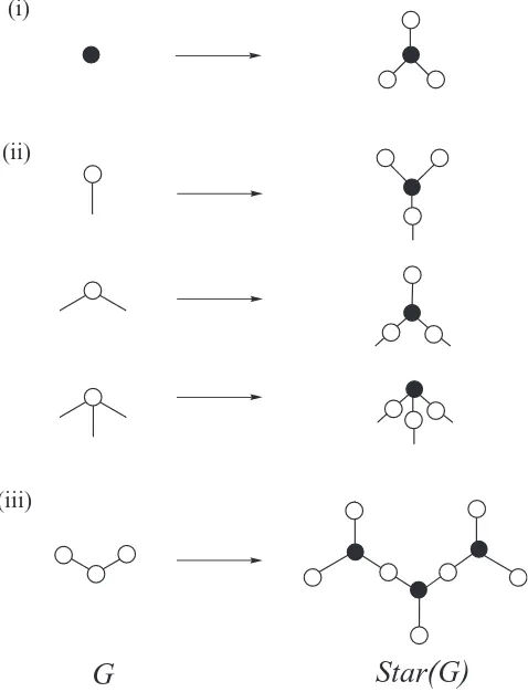
FIG. 3. The star construction. Starting from a parentG, (i) each vertex is replaced by a star graphS3; (ii) stars that are neighbours along an original edge ofGare fused at a peripheral vertex, leaving (3−d) pendent vertices per star replacing the original vertex of degreed.
a parent graph Gis replaced by a three-pointed star S3, and
pairs of stars corresponding to edges ofGare fused by super-position of a terminal vertex of each (see Figure3). Given that S3has three peripheral vertices, as the starting graph is
chem-ical (i.e., connected and with maximum degree ≤3) withn vertices andmedges, the derived graphStar(G) has 4n−m vertices and 3nedges of which 3n−2mare leaves, connect-ing central vertices of stars to vertices of degree 1. IfGhas adjacency eigenvalues {μi}, the graphStar(G) has 2n
eigen-values given by±√3+μi, with all other eigenvalues zero. Precisely in the case thatGis cubic and bipartite,Star(G) has two zero eigenvalues arising fromμn= −3 ofG. Hence, the
total number of zero eigenvalues ofStar(G) is 2n−m+2 for cubic bipartiteGand 2n−mfor all chemical graphs.
Application of the starification operation to all chemical graphs with 2<n<14 indicates that “nearly all”Star(G) for chemical parentsGare distinct omni-insulators. The “excep-tions” (Star(G) that are not distinct omni-insulators) are com-paratively rare: for parents withn=2, . . . 14, there are only 0, 0, 1, 1, 4, 4, 14, 23, 73, 166, 533, 1504, 5061, . . . excep-tions (to be compared with the much larger total numbers of chemical graphs listed in TableVII). Features common to the exceptions are under investigation. For example, some but not all cubic graphs Glead to exceptions, whereas all chemical treesGonnvertices lead to distinct omni-insulatorsStar(G) with 3n+1 vertices.
It is intriguing to ask exactly “why” the omni-insulating chemical trees have their characteristic property, and “why” in general insulation should be associated with high nullity. A hint comes from observations on calculated transmission in so-called cross-conjugated systems:11,39,40 a connection
across a cross-conjugated junction in model systems leads to strong reduction in transmission40 at energies that are
asso-ciated with the eigenvalues of the intervening side chain.39
Within the graph-theoretical version of the SSP model,13this
corresponds to a theorem that can be derived straightfor-wardly from our previous work on composite systems.17
Theorem 6.2. Let three fragments A, B, and C be
con-nected via a single three-coordinate vertex D to form a Y-shaped junction. The vertices adjacent to D in A, B, C are
wA,wB,andwC,respectively. If a device is constructed with ¯
L in A and R¯ in B, the opacity polynomial of the device, j2=ut −sv,is
j2(ABC)=j2(A)j2(B)φ2(C),
where j2(A) is the opacity polynomial for a device
consist-ing of A alone with connectionsL¯ andwA,j2(B)is the
opac-ity polynomial for a device consisting of B with connections
wB andR¯,and φ(C)is the characteristic polynomial of the
graph C.
Proof is by combination of Theorems 6 and 7 from our earlier paper.17 Our omniconducting trees include multiple
copies of such Y-junctions, and the denominator of the trans-missionT(E) will therefore contain zeroes atE=0 arising from the many leaves on these particular trees, as will the characteristic polynomial of the tree itself. This is suggestive of a more general connection between between nullity, cross-conjugation, and omni-insulation.
VII. CONCLUSIONS
It has been shown here that the graph theoretical SSP model leads naturally to the definition of omni-conductors and omni-insulators, that membership of the various cate-gories is crucially dependent on graph nullity (number of non-bonding orbitals) and is governed by a number of gen-eral theorems, and that many families of chemically relevant molecular graphs omni-conduct. For example, many bicyclic π-systems, and almost all fullerenes,33 are strong omnicon-ductors.
It will be interesting to see the extent to which these prop-erties are retained in more sophisticated models of molecular conduction.
ACKNOWLEDGMENTS
1A. K. Geim and K. S. Novoselov,Nat. Mater.6, 183 (2007). 2S. Houlton, Chem. World8, 65 (2011).
3M. Ratner,Nat. Nanotechnol.8, 378 (2013).
4D. Walter, D. Neuhauser, and R. Baer,Chem. Phys.299, 139 (2004). 5M. Ernzerhof, H. Bahmann, F. Goyer, M. Zhuang, and P. Rocheleau,J.
Chem. Theory Comput.2, 1291 (2006).
6G. Solomon, D. Andrews, R. Van Duyne, and M. A. Ratner,
ChemPhysChem10, 257 (2009).
7C. Herrmann, G. C. Solomon, J. E. Subotnik, V. Mujica, and M. A. Ratner,
J. Chem. Phys.132, 024103 (2010).
8Y. Zhou and M. Ernzerhof,J. Chem. Phys.132, 104706 (2010). 9A. Baratz and R. Baer,J. Phys. Chem. Lett.3, 498 (2012).
10V. Mujica, M. Kemp, and M. A. Ratner, J. Chem. Phys. 101, 6849 (1994).
11R. Collepardo-Guevara, D. Walter, D. Neuhauser, and R. Baer, Chem.
Phys. Lett.393, 367 (2004).
12F. Goyer, M. Ernzerhof, and M. Zhuang,J. Chem. Phys. 126, 144104 (2007).
13B. T. Pickup and P. W. Fowler,Chem. Phys. Lett.459, 198 (2008). 14M. Ernzerhof,J. Chem. Phys.127, 204709 (2007).
15M. Ernzerhof,J. Chem. Phys.135, 014104 (2011).
16P. W. Fowler, B. T. Pickup, and T. Z. Todorova,Chem. Phys. Lett.465, 142 (2008).
17P. W. Fowler, B. T. Pickup, T. Z. Todorova, and T. Pisanski,J. Chem. Phys.
130, 174708 (2009).
18P. Fowler, B. Pickup, T. Todorova, and W. Myrvold,J. Chem. Phys.131, 044104 (2009).
19P. Fowler, B. Pickup, T. Todorova, and W. Myrvold,J. Chem. Phys.131, 244110 (2009).
20F. Goyer and M. Ernzerhof,J. Chem. Phys.134, 174101 (2011). 21P. Rocheleau and M. Ernzerhof,J. Chem. Phys.137, 174112 (2012).
22D. Mayou, Y. Zhou, and M. Ernzerhof,J. Phys. Chem. C117, 7870 (2013). 23J. Sylvester, Philos. Mag.1, 295 (1851).
24I. Gutman and O. Polansky,Mathematical Concepts in Organic Chemistry
(Springer, Berlin, 1986).
25I. Sciriha, M. Debono, M. Borg, P. W. Fowler, and B. T. Pickup, Ars Math.
Contemp.6, 261 (2013).
26I. Sciriha and I. Gutman, Util. Math.54, 257 (1998).
27A. L. Cauchy,Oeuvres Complètes d’Augustin Cauchy (IIe Série)
(Gauthier-Villars et fils, Paris, 1882–1974), Tome 9, p. 174, Exer. de Math. 4 (1829).
28I. Sciriha,Discrete Math.181, 193 (1998).
29C. R. Johnson and B. D. Sutton,SIAM J. Matrix Anal. Appl. 26, 390 (2004).
30I. Sciriha, Util. Math.52, 97 (1997).
31I. Sciriha, Electron. J. Linear Algebra16, 451 (2007). 32I. Sciriha, Ars Math. Contemp.2, 217 (2009).
33P. W. Fowler, B. T. Pickup, T. Z. Todorova, R. D. L. Reyes, and I. Sciriha,
Chem. Phys. Lett.568–569, 33 (2013).
34P. W. Fowler and D. E. Manolopoulos,An Atlas of Fullerenes(Clarendon
Press, Oxford, 1995; Dover Publications, Inc., NY, 2006).
35G. Brinkmann and B. D. McKay, MATCH Commun. Math. Comput.
Chem.58, 323 (2007), see alsohttp://cs.anu.edu.au/~bdm/plantri. 36G. Brinkmann, O. D. Friedrichs, S. Lisken, A. Peeters, and N. V.
Cleem-put, MATCH Commun. Math. Comput. Chem.63, 533 (2010), see also http://caagt.ugent.be/CaGe.
37G. Brinkmann and A. W. M. Dress,J. Algorith.23, 345 (1997). 38A. Farrugia, J. B. Gauci, and I. Sciriha,Spec. Matrices1, 28–41 (2013). 39M. Ernzerhof, M. Zhuang, and P. Rocheleau,J. Chem. Phys.123, 134704
(2005).
40G. Solomon, D. Andrews, R. Goldsmith, T. Hansen, M. Wasielewski, R.