an example.
White Rose Research Online URL for this paper: http://eprints.whiterose.ac.uk/151748/
Version: Accepted Version
Article:
Gielen, S. orcid.org/0000-0002-8653-5430 (2014) Quantum cosmology of (loop) quantum gravity condensates : an example. Classical and Quantum Gravity, 31 (15). ISSN
0264-9381
https://doi.org/10.1088/0264-9381/31/15/155009
The final publication is available at IOS Press through http://dx.doi.org/10.1088/0264-9381/31/15/155009
[email protected] https://eprints.whiterose.ac.uk/ Reuse
Items deposited in White Rose Research Online are protected by copyright, with all rights reserved unless indicated otherwise. They may be downloaded and/or printed for private study, or other acts as permitted by national copyright laws. The publisher or other rights holders may allow further reproduction and re-use of the full text version. This is indicated by the licence information on the White Rose Research Online record for the item.
Takedown
If you consider content in White Rose Research Online to be in breach of UK law, please notify us by
arXiv:1404.2944v3 [gr-qc] 4 Jul 2014
condensates: An example
Steffen Gielen
Perimeter Institute for Theoretical Physics, 31 Caroline St. N., Waterloo, Ontario N2L 2Y5, Canada
E-mail: [email protected]
Abstract. Spatially homogeneous universes can be described in (loop) quantum gravity as condensates of elementary excitations of space. Their treatment is easiest in the second-quantised group field theory formalism which allows the adaptation of techniques from the description of Bose–Einstein condensates in condensed matter physics. Dynamical equations for the states can be derived directly from the underlying quantum gravity dynamics. The analogue of the Gross–Pitaevskii equation defines an anisotropic quantum cosmology model, in which the condensate wavefunction becomes a quantum cosmology wavefunction on minisuperspace. To illustrate this general formalism, we give a mapping of the gauge-invariant geometric data for a tetrahedron to a minisuperspace of homogeneous anisotropic 3-metrics. We then study an example for which we give the resulting quantum cosmology model in the general anisotropic case and derive the general analytical solution for isotropic universes. We discuss the interpretation of these solutions. We suggest that the WKB approximation used in previous studies, corresponding to semiclassical fundamental degrees of freedom of quantum geometry, should be replaced by a notion of semiclassicality that refers to large-scale observables instead.
1. Introduction
There is by now a variety of approaches to the problem of quantum gravity which are actively pursued [1]. Research into any of these directions generally addresses one of two basic aims. The first is to show that a proposed theory of quantum gravity is in itself consistent and that its objects are mathematically well-defined, computable, and can be translated into observable quantities, so that the theory can, at least in principle, be confronted with experiment. The second aim is a derivation of the phenomenology of the theory, which usually requires taking a ‘low-energy’ or ‘semiclassical’ regime, in which the theory should at least be consistent with present observational constraints on deviations from the predictions of general relativity and the standard model of particle physics. It is then often claimed that any genuine quantum-gravitational effect, going beyond separate predictions of general relativity or the standard model, would be intrinsically unobservable, since the Planck scale is many orders of magnitude above the energy scales probed in particle accelerators or hypothetical experiments. However, while it is indeed difficult to come up with present-day experiments that probe Planck-scale physics (for some efforts in this direction, see [2]), the very early universe provides a natural laboratory in which quantum gravity effects can be expected to play a role.
Inflation, the standard paradigm for the physics of the very early universe, has been spectacularly corroborated in the recent observations made by Planck [3] and BICEP2 [4]. However, despite its phenomenological success, there are several theoretical issues that remain open: the inflaton and its potential are not part of the standard model, and have to be added by hand. While inflation provides a picture in which the physics at the Big Bang singularity is not observationally relevant today, as its imprint has been stretched outside the causal horizon during the accelerated expansion, theorems such as [5] show that inflationary spacetimes have a past singularity, so that there is still a need for a more complete theory. Eternal inflation seems to have drastic and contentious theoretical consequences [6]. Observationally, the BICEP2 results seem to imply a violation of the Lyth bound [7]: the inflaton field presumably varies over super-Planckian scales during inflation. All of this motivates the study of quantum-gravitational models with regard to their predictions for cosmology.
Loop quantum gravity (LQG) has some of the structures one would expect in a full theory of quantum gravity: kinematical states corresponding to functionals of the Ashtekar–Barbero connection can be rigorously defined, and geometric observables such as areas and volumes are well-defined as operators, typically with discrete spectrum
[10]. Using the LQG formalism in quantising symmetry-reduced gravity leads to loop
quantum cosmology (LQC) [11]. Because of the structures of LQG, LQC allows a rigorous analysis of issues that could not be addressed within the Wheeler–DeWitt quantisation of conventional quantum cosmology, such as a definition of the physical inner product. Recently, LQC has made contact with CMB (cosmic microwave back-ground) observations, as the usual inflationary scenario is now discussed in LQC [12].
One missing ingredient in the formalism of LQC is its embedding into the full setting of LQG. Just as in conventional quantum cosmology, one has performed a symmetry reduction before quantisation, and truncated almost all degrees of freedom present in the full Hilbert space of LQG. A different approach aiming at a more complete picture would be to work within the full Hilbert space, identify states that can represent macroscopic, (approximately) spatially homogeneous universes, and extract information about their dynamics. Clearly, this last step will involve many approximations, but since these are approximations for equations of the full theory, one has some control about the error made. Already the identification of suitable states that represent cosmological spacetimes is challenging in a theory like LQG: because of the notion of background independence built into the definition of the theory, the most natural notion of vacuum state is the ‘no space’ state, which has zero expectation value for geometric observables (areas, volumes, etc). Elementary excitations over this vacuum are usually interpreted as distributional geometries, and a macroscopic nondegenerate configuration is unlikely to be found as a small perturbation of this vacuum.
A new approach towards addressing the issue of how to describe cosmologically
relevant universes in (loop) quantum gravity was recently proposed in [13, 14] ‡. This
proposal uses the group field theory (GFT) formalism, itself a second quantisation
formulation of the kinematics and dynamics of LQG [16]: one has a Fock space of LQG spin network vertices (or tetrahedra, as building blocks of a simplicial complex),
annihilated and created by the field operator ˆϕ and its Hermitian conjugate ˆϕ†,
respectively. The advantage of using this reformulation is that field-theoretic techniques are available, as a GFT is a standard quantum field theory on a curved (group)
manifold (not to be interpreted as spacetime). In particular, one can define coherent
or squeezed states for the GFT field, analogous to states used in the physics of Bose–
Einstein condensates or in quantum optics; these representquantum gravity condensates.
They describe a large number of degrees of freedom of quantum geometry in the same microscopic quantum state, which is the analogue of homogeneity for a differentiable metric geometry. This idea was made explicit in [14]: after embedding a condensate of tetrahedra into a smooth manifold representing a spatial hypersurface, one shows that
the spatial metric (in a fixed frame) reconstructed from the quantum state is compatible with spatial homogeneity. As the number of tetrahedra is taken to infinity, a continuum homogeneous metric can be approximated to a better and better degree.
At this stage, the condensate states defined in this way are kinematical. They are gauge-invariant (locally Lorentz invariant) by construction, and represent geometric data invariant under (active) spatial diffeomorphisms, but they do not satisfy any dynamical equations corresponding to a Hamiltonian constraint in geometrodynamics. The strategy followed in [13, 14] for extracting information about the dynamics of these states is the use of Schwinger–Dyson equations of a given GFT model. These give
constraints on the n-point functions of the theory evaluated in a given condensate state
(approximating a non-perturbative vacuum), which can be translated into differential equations for the ‘condensate wavefunction’ used in the definition of the state. Again, this is analogous to condensate states in many-body quantum physics, where such an expectation value gives, in the simplest case, the Gross–Pitaevskii equation for the condensate wavefunction. The truncation of the infinite tower of such equations to the simplest ones is part of the approximations made. As argued in [13, 14], the
effective dynamical equations thus obtained can be viewed as defining a quantum
cosmology model, with the condensate wavefunction interpreted as a quantum cosmology wavefunction. This provides a general procedure for deriving an effective cosmological
dynamics directly from the underlying theory of quantum gravity. In a specific
example, it was shown how a particular quantum cosmology equation of this type, in a semiclassical WKB limit and for isotropic universes, reduces to the classical Friedmann equation of homogeneous, isotropic universes in general relativity.
The purpose of this paper, apart from reviewing the formalism introduced in detail in [14], is to analyse more carefully the quantum cosmological models derived from quantum gravity condensate states in GFT. In particular, the formalism identifies the gauge-invariant configuration space of a tetrahedron with the minisuperspace of homogeneous (generally anisotropic) geometries. We will justify this interpretation and propose a convenient set of variables for the gauge-invariant geometric data, which can be mapped to the variables of a general anisotropic Bianchi model (for which the metric is not diagonalised and has six components). We will then revisit the example that led to the Friedmann equation in [13, 14] and study it directly as a quantum cosmology equation, without a WKB limit. The Friedmann equation arising in a WKB limit in [13] appeared to have no solutions, as there was a mismatch between the curvature of the gravitational connection, assumed to be small on the scale of the tetrahedra, and the spatial curvature term which was large on the same scale. Here we find simple solutions to the full quantum equation, corresponding to isotropic universes. They can only satisfy the condition of rapid oscillation of the WKB approximation for large positive values of
the coupling µin the GFT model. Forµ <0, states are sharply peaked on small values
2. From quantum gravity condensates to quantum cosmology
Here we review the relevant steps in the construction of effective quantum cosmology equations for quantum gravity condensates. We work in the group field theory (GFT) formalism, which is a second quantisation formulation of loop quantum gravity spin networks (of fixed valency), or their dual interpretation as simplicial geometries. For full details of the precise relation between the two, see [16].
The basic structures of the GFT formalism in four dimensions are a complex-valued
field ϕ :G4 →C, satisfying a gauge invariance property
ϕ(g1, . . . , g4) =ϕ(g1h, . . . , g4h) ∀h∈G , (1)
and the basic (non-relativistic) commutation relations imposed in the quantum theory
[ ˆϕ(gI),ϕˆ†(gI′)] = 1G(gI, gI′), [ ˆϕ(gI),ϕˆ(gI′)] = [ ˆϕ†(gI),ϕˆ†(gI′)] = 0. (2)
The relations (2) are analogous to those of non-relativistic scalar field theory, where the
mode expansion of the field operator defines annihilation operators, ˆφ(~x) = P
kˆakφk(~x),
and similarly for the Hermitian conjugate ˆφ†(~x) = P
kˆa
†
kφk(~x). In GFT, the domain of
the field(s) is four copies of a Lie groupG, interpreted as the local gauge group of gravity,
which can be taken to beG= Spin(4) for Riemannian andG= SL(2,C) for Lorentzian
models. In loop quantum gravity, the gauge group is the one given by the classical
Ashtekar–Barbero formulation, G= SU(2). The property (1) encodes invariance under
gauge transformations acting on spin network vertices, as we will see shortly. In (2),1G
is an identity operator on the group compatible with (1). For compact G,
1G(gI, gI′) = Z G dh 4 Y I=1
δ(gIh(gI′)−1), (3)
where here and in the following the measure dh is normalised to R
dh= 1.
One then defines a Fock vacuum |∅i annihilated by all ˆϕ(gI), analogous
to the diffeomorphism-invariant Ashtekar–Lewandowski vacuum of LQG, with zero
expectation value for all area or volume operators. The conjugate ˆϕ†(g
I) acting on
|∅i creates a GFT ‘particle’, interpreted as a 4-valent spin network vertex or a dual
tetrahedron:
ˆ
ϕ†(g
1, g2, g3, g4)|∅i=| • i
✂ ✂ ✂ ✂ ✂ ✂ ✂ ✂ ✂✂✏✏✏✏ ✏✏✏✏ ✏ ❅ ❅ ❅ ❅ ❅ ❅ ❅ ❅ ❅ ❅ ❅ ❅ ❅ ❅ ✂ ✂ ✂ ✂ ✂ ✂✂ g1 g2 g3 g4 (4)
The geometric data attached to this tetrahedron, four group elements gI ∈ G, is
interpreted as parallel transports of a (gravitational) connection along links dual to the four faces. Gauge transformations act on the vertex where these links meet as
The LQG interpretation of (4) is that of a state that fixes the parallel transports of
the Ashtekar–Barbero connection to begI along the four links given by the spin network,
while they are undetermined everywhere else. Again, this is analogous to the Fock space
of usual scalar field theory in which |~xi= ˆφ†(~x)|0i defines a particle at position ~x.
In the canonical formalism of Ashtekar and Barbero, the canonically conjugate
variable to the connection is a densitised (inverse) triad, with dimensions of area, that
encodes the spatial metric. The GFT formalism can be translated into this ‘momentum
space’ formulation by use of a non-commutative Fourier transform [17],
˜
ϕ(B1, . . . , B4) = Z
(dg)4
4 Y I=1
egI(BI)ϕ(g1, . . . , g4) (5)
where egI(BI) is a choice of plane wave on G. Since G is non-Abelian, the product
of plane waves defined by eg(B)⋆ eg′(B) = egg′(B) is non-commutative; its extension
to general superpositions of plane waves turns the space parametrised by BI into a
non-commutative geometry, which is the Lie algebra g⊕4 of G4.
The geometric interpretation of the variables BI ∈ g is as geometric bivectors
associated to a spatial triade, defined by the integral R
△Ie
A∧eB over a face △
I of the
tetrahedron. Hence, the one-particle state
|B1, . . . , B4i= ˆ˜ϕ(B1, . . . , B4)|∅i (6)
defines a tetrahedron with minimal uncertainty in the ‘fluxes’,i.e. oriented area elements
R
△Ie
A∧eB, given by B
I. § Again, in the LQG interpretation this state completely
determines the metric variables for one tetrahedron, while being independent of all other degrees of freedom of geometry in a spatial hypersurface.
The idea of quantum gravity condensates is to use many excitations over the
Fock space vacuum |∅i, all in the same microscopic configuration, to better and
better approximate a smooth homogeneous metric (or connection), as a many-particle state can contain information about the connection and the metric at many different points in space. Choosing this information such that it is compatible with a spatially
homogeneous metric while leaving the particle number N free, the limit N → ∞
corresponds to a continuum limit in which a homogeneous metric geometry is recovered. In the simplest case, the definition for GFT condensate states is
|σi:=N(σ) exp (ˆσ)|∅i with σˆ:=
Z
(dg)4 σ(gI) ˆϕ†(gI), (7)
whereN(σ) is a normalisation factor. The exponential creates a coherent configuration
of many building blocks of geometry. At fixed particle number N, a state of the form
ˆ
σN|∅i would be interpreted as defining a metric (or connection) that looks spatially
homogeneous when measured at the N positions of the tetrahedra, given an embedding
into space. However, one does not work at fixed particle number, but there is a sum over all possible particle numbers. The condensate picture is rather different from many constructions in the literature: it does not use a fixed graph or discretisation of space.
The above summary gives an intuitive picture rather than full details, which can be found in [14]. It uses the geometric interpretation of LQG spin network states, which is obtained by viewing LQG as a quantisation of a classical action for general relativity. Ultimately, the identification of the degrees of freedom of the quantum theory with classical geometric quantities involves a detailed understanding of the continuum limit, which is largely an open issue [19]. Computing an effective dynamics for the reconstructed macroscopic ‘metric’, and verifying whether it satisfies Einstein’s equations (with higher curvature corrections), would be an important step in this direction. GFT condensates can address this question in the case of spatial homogeneity. While spatial homogeneity requires that all elementary building blocks of geometry are in the same microscopic configuration, it does not state what the elementary building blocks are. A natural second type of condensate is a condensate of ‘molecules’ of two tetrahedra, with pairwise identified faces. It is defined by
|ξi:=N(ξ) expξˆ|0i, ξˆ:= 1
2
Z
(dg)4(dh)4 ξ(g−1
I hI) ˆϕ†(gI) ˆϕ†(hI). (8)
In terms of LQG spin networks, the elementary building block of (8) is a ‘dipole’ graph for which the four links going out of one vertex all meet at a second vertex, thus forming a gauge-invariant closed spin network. Indeed, using (1), the condensate wavefunction
ξ in (8) is separately invariant under two gauge transformations,
ξ(g1, . . . , g4) =ξ(kg1k′, . . . , kg4k′) ∀k, k′ ∈G . (9)
These transformations are local gauge transformations in the geometric interpretation of the GFT variables, acting respectively on the vertex of the tetrahedron in (4) and on its boundary (contracted to a second vertex for the dipole). In terms of the dual Lie algebra variables, the first type of transformation means that the bivectors add to zero,
P4
I=1BI = 0, while the second one is a gauge transformation BI 7→kBIk−1.
In order to only depend on geometric variables and not on a local choice of Lorentz frame, the condensate must be invariant under both sets of transformations. Hence, in
the case of (7), we impose that σ(gI) =σ(k gI)∀k∈G.
In both cases, the GFT condensate is defined in terms of a wavefunction on G4
invariant under separate left and right actions of G on G4. The strategy introduced in
[14] is then to demand that the condensate solves the GFT quantum dynamics, expressed
in terms of the Schwinger–Dyson equations which relate different n-point functions for
the condensate. An important approximation is to only consider the simplest Schwinger– Dyson equations, which will give equations of the form
ˆ
Kσ(g1, . . . , g4) +
ˆ
Vσ(g1, . . . , g4) = 0, (10)
where ˆK is a linear (potentially nonlocal) differential operator, and ˆVσ can be a
potential terms in the GFT action. This is again analogous to the case of the Bose– Einstein condensate where the simplest equation of this type (the expectation value of the classical equation of motion) gives the Gross–Pitaevskii equation.
In the case of a real condensate, the condensate wavefunction Ψ(~x), corresponding to a nonzero expectation value of the field operator, has a direct physical interpretation: expressing it in terms of amplitude and phase, Ψ(~x) =pρ(x)e−iθ(~x), one can rewrite the Gross–Pitaevskii equation to discover thatρ(x) and~v(x) =∇θ(~x) satisfyhydrodynamic equations in which they correspond to the density and the velocity of the quantum fluid defined by the condensate. Microscopic quantum variables and macroscopic classical variables are directly related.
The wavefunction σ(gI) orξ(gI) of the GFT condensate should play a similar role.
It is not just a function of the geometric data for a single tetrahedron, but equivalently a function on aminisuperspaceof spatially homogeneous universes. The effective dynamics for it, extracted from the fundamental quantum gravity dynamics given by a GFT model, can then be interpreted as a quantum cosmology model. The resulting quantum cosmology equations are in general nonlinear, which extends the usual formalism of Schr¨odinger-type linear equations but has been proposed in a different context before
[20]. In the rest of this paper, we will make the interpretation of these equations as
quantum cosmology models more explicit, and study a concrete example.
3. Minisuperspace = gauge-invariant configuration space of a tetrahedron
Condensate states of the type discussed are determined by a wavefunction σ, which is
a complex-valued function on the space of four group elements (for given gauge group
G) which is invariant under
σ(g1, . . . , g4) = σ(kg1k′, . . . , kg4k′), k, k′ ∈G , (11)
and hence really a function on G\G4/G. This quotient space is a smooth manifold
with boundary, without a group structure. It is the gauge-invariant configuration
space of the geometric data associated to a tetrahedron or, perhaps more naturally, of a ‘dipole’ configuration of two tetrahedra with pairwise identified faces. When the effective quantum dynamics of GFT condensate states is reinterpreted as (perhaps
nonlinear) quantum cosmology equations, G\G4/G becomes a minisuperspace of
spatially homogeneous geometries.
For consistency, the dynamics given by ˆK and ˆV in (10) must be compatible with
the symmetries of σ, given by the left and right action of G on G4,
[ ˆK, Lk] = [ ˆK, Rk′] = 0, k, k′ ∈G , (12)
and similar for ˆV. These operators then act on the Hilbert space of condensate
wavefunctions defined on G\G4/G.
To proceed, we note that there is a natural bijection of quotient spaces,
with inverse
β−1: G3/Ad
G →G\G4/G , [g1, g2, g3]7→[g1, g2, g3, e], (14)
where AdG is the adjoint action of G on G3 which maps gi 7→ kgik−1. Hence one can
equivalently view σ as a function on G3/Ad
G. Its non-commutative Fourier transform
˜
σ(B1, B2, B3) = Z
(dg)3 σ(g1, g2, g3) 3 Y
i=1
egi(Bi) (15)
satisfies ˜σ(B1, B2, B3) = ˜σ(kB1k−1, kB2k−1, kB3k−1) for all k ∈G, due to the property
ekgk−1(B) = eg(k−1Bk) of the plane waves [17], and is thus a function on g⊕3/AdG ≡
(Lie(G3))/Ad
G. This latter quotient space is closely related to the space of homogeneous
spatial metrics: any homogeneous metric is specified by giving a group action on a manifold, and fixing the metric at one point in the manifold. Focussing on non-degenerate metrics, spatially homogeneous metrics are in one-to-one correspondence to
elements of the homogeneous space GL(3)/O(3)≃SL(3)/O(3)×(R\{0}) (see e.g. [21]
for this and more general properties of the superspace of 3-metrics).
As a vector space, g⊕3 is just Rdim(G)×3. Choosing G = SU(2) and assuming
the non-degeneracy condition Tr(B1B2B3) 6= 0 means restricting to the subspace
GL(3)/AdSU(2) ⊂ R3×3/AdSU(2). The orbits of the action SU(2) on this space are
smaller than the orbits of O(3), as they preserve the sign of the invariant Tr(B1B2B3).
Restricting to Tr(B1B2B3)>0, i.e. making a choice of orientation, the domain of σ in
(15) is indeed just the space of (non-degenerate) homogeneous 3-metrics.
The above is not just a topological identification of quotient spaces, but follows from the geometric interpretation of the GFT data attached to tetrahedra, or pairs of
tetrahedra. As anticipated above, the Lie algebra elements BI are interpreted as the
discretised analogue of a triad of 1-forms eA,
BIAB ∼
Z
△I
eA∧eB. (16)
One of the assumptions of GFT condensates is that the discrete BAB
I are a good
approximation to a continuum homogeneous metric, which can then be reconstructed from the geometric data in the GFT states. One hence assumes the reconstructed geometry to be almost constant over the scale of the tetrahedra, so that one can define
BiAB =:ǫijkeAj eBk (17)
with the eA
j defining a ‘triad’ at a given reference point (e.g. one of the vertices) of a
tetrahedron. Assuming nondegeneracy, the space of such ‘triads’ is GL(3), and its
gauge-invariant data corresponds to elements of GL(3)/O(3); the Bi then simply correspond
to the densitised inverse triad of LQG.
If the GFT gauge group G is chosen to be a four-dimensional rotation group such
as SL(2,C), the identification of variables is more subtle. (17) is no longer a definition
of eA
i , as there need not be a set of vectors eAi for given Bi ∈ g so that (17) holds.
constraints which restrict the modes appearing in the Peter–Weyl expansion of the GFT field in representations ofG(for a review of various prescriptions in the spin foam language, see [22]). In the GFT formalism, this can be done at the level of the field
itself, or in the action, either in the kinetic or the potential term, see e.g. [23].
Geometrically, the role of simplicity constraints is to select a local SU(2) subgroup
of G at each point in a spatial hypersurface; this can be understood as ‘spontaneous
symmetry breaking’ by a field ofobserverswith respect to which a local SU(2) subgroup
is defined [24]. A gauge-fixing with constant observer field leads to the Ashtekar–Barbero formulation in terms of SU(2); conversely, the Lorentz-covariant theory can be recovered from the SU(2) theory by specifying how it transforms under changes of observer.
In the GFT quantum analogue of this classical formalism, instead of starting with
a larger gauge group G and restricting representations, one can choose G= SU(2) and
implement simplicity constraints through a choice of embedding map
̟ : L2(SU(2)4/SU(2)) →L2(H4/H) (18)
whereH = Spin(4) orH = SL(2,C). This embedding map is the analogue of a classical
choice of observer at each point in a spatial hypersurface which determines an embedding
of SU(2) into G. Its choice is not unique and different choices for ̟ correspond to
different spin foam models, see [14]. Here we assume that a suitable map ̟ can be
chosen, and one can work in Ashtekar–Barbero-type variables withG= SU(2).
Having established that an open connected subset of su(2)⊕3/AdSU(2) represents
the space of nondegenerate homogeneous 3-metrics, we fix the coordinates
Bij :=−
1
2Tr (BiBj) =B~i·B~j, (19)
which is a global coordinate system. In the last equation, we have identified su(2)≃R3
using the standard basis of Pauli matrices, i.e. B =: i~σ·B~ forB ∈su(2).
In terms of the components of the spatial metric, using (17), the function Bij
corresponds to the minor of the entrygij of the spatial metricgdefined bygij =δABeAi eBj :
B11=g22g33−g232 , etc. (20)
We note that for detg 6= 0, gij is diagonal if and only if Bij is diagonal. detg can be
computed by considering
detBij =
1 6ǫ
ijkǫlmnB
ilBjmBkn= (detg)2. (21)
Note that g, like Bij, is by construction positive (semi-)definite, and detg 6= 0 or
detBij 6= 0 is equivalent to the Bi being linearly independent, and forming a basis of
su(2) ≃ R3. The space of non-degenerate matrices Bij is then again the homogeneous
space GL(3)/O(3) ≃ SL(3)/O(3) × (R\{0}), where the R\{0} corresponds to an
(oriented) overall volume factor, which we may restrict to be positive.
In these variables, having an isotropic universe, i.e. a 3-metric proportional to the
So far, we have treated su(2)⊕3/AdSU(2) only as a vector space, ignoring its Lie
algebra structure. Using the basic commutation relations {B~i, ~Bj}= Gδij(B~i×B~j),
{Bij, Bkl}= G Tr(B1B2B3)(ǫiljδjk+ǫjliδik+ǫikjδjl+ǫjkiδil) ; (22)
the quotient su(2)⊕3/AdSU(2) inherits a non-commutative structure from su(2).
Expressed in terms of Lie algebra variables in su(2)⊕3/AdSU(2), effective quantum
cosmology models derived from GFT condensates naturally describe anon-commutative
quantum cosmology, with some similarity to models such as [25]. Here G is a
dimensionful parameter which in LQG is normally a product of Newton’s constant
with a numerical factor, perhaps involving the Barbero–Immirzi parameter γ, and so
corresponds to an inverse tension [26]. We also note that the coordinates Bii commute
with all others; noncommutativity becomes only relevant for terms at least quadratic in anisotropies, and could be ignored if one linearises around isotropy.
To extend the discussion to connection variables, we need to choose a convenient
set of coordinates on SU(2)3/Ad
SU(2) which can be interpreted in terms of quantum
cosmology. Recall that one interprets the elements of SU(2) as parallel transports of a gravitational connection which is taken as approximately constant over the scale of the tetrahedra,
g =:Pexp
Z e
ω=Pexp
Z ν 0
dxiωi ≈exp(ν ωx), (23)
if the coordinate system (on the spatial manifold) is chosen such that the edge e has
coordinate length ν in the x direction. The adjoint action AdSU(2) on g then becomes
ωx 7→ kωxk−1, which corresponds to an SU(2) gauge transformation that is constant
over e (as is consistent with the assumption of constant ω). Of course, as SU(2) is
compact, and hence there are nonzero T ∈ su(2) for which exp(T) = e, there is no
invertible mapg 7→ω[g] that would allow a reconstruction of the ‘connection’ω from its
parallel transports. At least in a neighbourhood of the identity in SU(2), we can write
g =p1−~π[g]21−i~σ·~π[g], |~π| ≤1, (24)
which defines coordinates ~π on SU(2). Comparing with (23), we have
~π =−~ωxsin(ν|~ωx|)/|~ωx|, (25)
again using su(2) ≃ R3, so that ~π corresponds to a ‘sine of the connection’. It is
the natural variable arising from a discretisation of a (gravitational) connection, and replaces the connection in the holonomy corrections of loop quantum cosmology [11].
The adjoint action of SU(2) on itself acts as rotations of the ‘coordinate vector’ ~π.
These coordinates are particularly useful if the Fourier transform (15) is defined by
eg(B) := exp(2iTr(gB)/~G), since this becomes simplyeg(B) = exp(i~π[g]·B/~ ~G). This
does not mean, of course, that the Fourier transform is the standard one on R3: there
is a non-trivial measure factor in (15), dg = d~π(1−~π2)−1/2. The coordinates ~π on the
group and B~ on the Lie algebra arenotcanonically conjugate as phase space variables,
phase spaceT∗G=G×g, where G is a non-Abelian Lie group, the Poisson bracket for
the Lie algebra variables is induced by the Lie bracket,
{Bα, Bβ}=cαβγBγ. (26)
A putative choice of coordinates pα on the group such that {pα, Bβ} ∝δαβ is then not
compatible with the Jacobi identity, as one would have
0=? {{Bα, Bβ}, pγ}+ permutations∝cαβγ. (27)
From the same argument, one sees that the first correction to {pα, Bβ} = c δαβ +. . .
comes in at linear order inp. The coordinates~πused in the following have this property:
they are canonically conjugate to the B~ (including, for dimensional reasons, a factor of
G) up to terms of linear and higher order in~π k. In the definition of GFT condensates,
we have assumed that gauge-invariant combinations of parallel transports are peaked on values close to the identity, which is a sufficient condition for guaranteeing that all components of the curvature remain small on the scale of the individual tetrahedra. This
is the regime in which |~π| ≪1 and~π and B~ can be viewed as canonically conjugate.
We then choose the invariants under the left and right actions of SU(2) on SU(2)4
πij :=~π[gig4−1]·~π[gjg−41], (28)
with |πij| ≤ 1 and πii ≥ 0, to define a coordinate system in a neighbourhood of the
identity [e, e, e]∈SU(2)3/Ad
SU(2). The coordinates~π cover a hemisphere ofS3 ∼SU(2)
for each of the three copies of SU(2), mapping it to a three-ball B3 ⊂ R3, and π
ij
are invariant under the adjoint action of SU(2) acting as rotations of R3. Note that
the identity coset [e, e, e]∈SU(2)3/Ad
SU(2) is in the boundary of SU(2)3/AdSU(2), as it
corresponds to a fixed point of AdSU(2): [e, e, e] = (e, e, e) P.
By (25), these coordinates correspond to gauge-invariant (in the sense explained above) combinations of the components of a ‘gravitational connection’ as follows,
πii= sin2(ν|~ωi|), πij = cosθijsin(ν|~ωi|) sin(ν|~ωj|), (29)
where θij is the angle between the connection components ~ωi and ~ωj again viewed as
elements of R3. We will later be interested in the isotropic case where only πii6= 0.
4. The example: Laplace–Beltrami beyond the WKB approximation
As an example of how effective quantum cosmology equations can be extracted from the dynamics of quantum gravity condensates, the discussion of [13, 14] considered
ˆ
K=
4 X
I=1
∆gI +µ , Vˆ = 0, (30)
where ∆g is the Laplace–Beltrami operator on SU(2) ∼ S3, and µ ∈ R. The choice
ˆ
V = 0 can arise from a condensate of the ‘dipole’ type for which it was shown that, for
a class of GFT potentials, the nonlinear term can be approximately neglected in the effective quantum cosmology equation. The choice of a Laplacian in the kinetic term can be motivated, among other arguments, by results in the renormalisation of GFT that suggest that such a kinetic term is generated by radiative corrections [28]. Its presence is used to define a notion of scale for a renormalisation group flow in GFT [29].
Let us consider (30) as an example, and explicitly reduce the quantum cosmology
equation from SU(2)4 to the variables π
ij invariant under separate left and right actions
of SU(2). It is immediate to see that (30) satisfies (12), as the Laplace–Beltrami operator
on SU(2) (defined with respect to the round metric on S3) is bi-invariant. In terms of
the coordinates~π on SU(2), ∆ is defined by
∆gf(π[g]) = (δαβ −παπβ)∂α∂βf(π)−3πα∂αf(π). (31)
On functions on SU(2)4/SU(2) which can be identified as functions on SU(2)3, using
the bijection [g1, g2, g3, g4]7→(g1g4−1, g2g4−1, g3g4−1), we can compute (in everything that
follows, there is no summation convention for indices i, j, k, l which run from 1 to 3)
4 X
I=1
∆gIσ(g1g
−1
4 , g2g−41, g3g4−1)
= X
i
∆giσ(g1g
−1
4 , g2g4−1, g3g4−1) + ∆g4σ(g1g
−1
4 , g2g4−1, g3g4−1)
= 2X
i
(δαβ −πiαπiβ)∂αi∂βi −3πiα∂αiσ(~π[gig−41])
+X
i6=j
q
1−~π2
i q
1−~π2
j +~πi·~πj
δαβ
−ǫαβγπγi q
1−~π2
j +ǫαβγπjγ q
1−~π2
i −παjπ β i
∂αi∂βjσ(~π[gig4−1]) (32)
where ~πi := ~π[gig4−1]. The Laplace–Beltrami operator with respect to g4 gives two
contributions, one which just doubles the other three contributions (which themselves
directly follow from right-invariance of ∆gi), and one which is ‘anisotropic’. (32) is
manifestly invariant with respect to the left SU(2) action ~πi 7→O~πi.
We now take σ to be a function on SU(2)3/Ad
SU(2), i.e. a function that only
depends on the coordinates πij, σ(~π[gig4−1]) = σ(π(ij)). As usual, round brackets denote
symmetrisation, making explicit that there are really only six independent coordinates
π(ij), as π(12) and π(21) refer to the same coordinate. Then, using the chain rule
∂αi∂βjσ(π(ij)) = X
k,l
πkαπlβ
∂2σ
∂π(ik)∂π(jl)
+X
k
πiαπkβ
∂2σ
∂πii∂π(jk)
+X
k
πkαπjβ
∂2σ
∂π(ik)∂πjj
+πiαπjβ
∂2σ
∂πii∂πjj
+δαβ
∂σ ∂π(ij)
+δαβδij
∂σ ∂πii
the action of P4
I=1∆gI onσ becomes
4
X
I=1
∆gIσ(πij)
= 2 X
i,k,l i6∈{k,l}
(π(kl)−π(ik)π(il))
∂2σ ∂π(ik)∂π(il)
+ 8X
i6=k
π(ik)(1−πii)
∂2σ ∂πii∂π(ik)
+ 8X
i
πii(1−πii)
∂2σ ∂π2
ii
+ 4X
i
(3−4πii)
∂σ ∂πii −
4X
i6=j
π(ij) ∂σ ∂π(ij)
+X
i6=j "
X
k,l
√ 1−πii
p
1−πjjπ(kl)+π(ij)π(kl)
−2p1−πjjπ[kli]−π(jk)π(il)
∂2σ
∂π(ik)∂π(jl)
(34)
+ 2X
k
√ 1−πii
p
1−πjjπ(ik)−π[ijk]
√ 1−πii
∂2σ
∂πii∂π(jk)
+ √1−πii p
1−πjjπij
∂2σ ∂πii∂πjj
+ 3√1−πii p
1−πjj
∂σ ∂π(ij)
.
This is now expressed only in terms of the coordinates π(ij), except for π[ijk] := ~πi·(~πj×~πk). Up to a sign, this can be reconstructed from
π2
[ijk]= det
πii πij πik
πij πjj πjk
πik πjk πkk
. (35)
This sign is a choice of orientation of the three vectors {~πi}which can not be obtained
from the O(3) invariant combinations ~πi ·~πj. As above, the space of non-degenerate
matrices {πij}, for which the determinant in (35) is non-vanishing, is GL(3)/O(3) ≃
SL(3)/O(3)×(R\{0}) which splits into two connected components. The coordinates
πij only parametrise one of these, and we can choose the component with π[123] >0.
(34) is the explicit expression of P4
I=1∆gIσ(πij) in the coordinates π(ij) on
SU(2)\SU(2)4/SU(2). Substituting (34) into (P4
I=1∆gI +µ)σ(π(ij)) = 0 defines a
homogeneous, anisotropic quantum cosmology model for an empty universe without matter. As suitable explicit solutions to it are difficult to construct, the strategy adopted in [14] was to go to a WKB limit: assume that
σ(π(ij)) =A(π(ij)) exp iS(π(ij))/~G
(36)
where S(π(ij)) oscillates rapidly compared to A(π(ij)), take the limit of ~G→0, define
the momentum B(ij) =∂S/∂π
(ij) conjugate toπ(ij), and interpret the resulting classical
equation for π(ij) and B(ij) in terms of gravitational dynamics. In the isotropic case,
this led to a holonomy-corrected Friedmann equation for vacuum Riemannian gravity,
whereP was identified with sin(ν ω) for the gravitational connectionω, for someν ∈R
+, and k > 0 is a constant interpreted as spatial curvature. This effective Friedmann
equation seemed to have no solutions, as a consistent approximation of a continuum metric by discrete building blocks seemed to require P ≪1, while k is a dimensionless ratio of WKB variables depending on the state and of O(1).
If (37) were the Friedmann equation for continuum variables, one could change
coordinates to rescale k, but this freedom is not present here: the geometric variables
are expressed with respect to the scale given by the discrete building blocks of geometry.
While in the identificationP = sin(ν ω) bothνandω depend on a choice of coordinates,
P does not; its value is fixed by properties of the tetrahedra in the condensate. The
issue that P ≪1 contradicts (37) cannot be resolved by changing coordinates.
Here we address two possible issues with the WKB analysis. The first is that the assumption of semiclassicality excludes many potentially interesting solutions. Generic quantum gravity condensates are not semiclassical at all, and it may not be meaningful to look for states that have semiclassical properties at the Planck scale. Large-scale observables should display semiclassical behaviour to agree with what we see, but this requirement may be different from the very simple WKB criterion on the condensate wavefunction, which would impose semiclassical behaviour already on the microscopic degrees of freedom. Our results in this section support the viewpoint, coming also from full quantum gravity, that the latter is not a physically meaningful assumption.
The second issue is technical. The WKB approximation in [14] was done at the level
of SU(2)4, with the symmetries of the wavefunction translated into relations among the
WKB variables, which were then substituted into the WKB equations. It is not clear whether this is equivalent to first reducing the quantum equation by using symmetries and then only introducing WKB variables for the gauge-invariant quantities.
To extend the analysis of [13, 14], we avoid a WKB approximation, and derive
analytical solutions to the quantum equation (P4
I=1∆gI +µ)σ(π(ij)) = 0. We consider
isotropic states for which σ only depends on the coordinates πii. Then from (34),
4 X I=1
∆gIσ(π(ij)) = 8 X
i
πii(1−πii)
∂2σ
∂π2
ii
+ 4X
i
(3−4πii)
∂σ ∂πii
+ 4X
i6=j
√
1−πii
p
1−πjjπ(ij)
∂2σ
∂πjj∂πii
. (38)
Due to the appearance of off-diagonal π(ij) in the second term, the only solution to
(P4
I=1∆gI +µ)σ(πii) = 0 compatible with our ansatz seems to be
σ(πii) =σ1(π11) +σ2(π22) +σ3(π33) (39)
with all σi separately satisfying
2p(1−p)σi′′(p) + (3−4p)σ′i(p) +µiσi(p) = 0 (40)
+ If we (tentatively) identify ω with the Ashtekar–Barbero conncetion, in the LQC notation of [11]
we would have P = sin(δ c) where δ can be a constant or depend on phase space variables. We will investigate the precise relation of the variables (π(ij), B(ij)) to the phase space variables of LQC more
for some µi such that Piµi = 14µ. Hence, all solutions that only depend on diagonal
elements πii can be obtained as a sum of solutions to the ordinary differential equation
2p(1−p)σ′′(p) + (3−4p)σ′(p) + ˆµ σ(p) = 0. (41)
Since (39) completely decouples π11, π22 and π33, let us now setσ2 =σ3 = 0, and leave
ˆ
µ arbitrary (one could set ˆµ= 1
4µ). We can then first compare (41) to the Friedmann
equation obtained in the WKB limit in [13, 14]. The WKB limit of (41) gives simply
2p(1−p) =O(~G), (42)
and hence p ≈ 0 or p ≈ 1. p can be identified with sin2(ν ω), and so again this is a
vacuum Friedmann equation, either for a flat or for a closed universe. Only p ≈ 1 is
compatible with the previous result (37); the solution p≈0, describing a flat universe,
appears when taking the WKB limit only for isotropic, gauge-invariant variables. We can now compare this approximation to the explicit general solution to (41),
σ(p) =χ4
r
1−p
p P 1 2 1 2( √
1+2ˆµ−1)(2p−1) +υ
4
r
1−p
p Q 1 2 1 2( √
1+2ˆµ−1)(2p−1),(43)
where Pm
n (x) and Qmn(x) denote associated Legendre functions of the first and second
kind, respectively, and χ and υ are constants.
One might worry about regularity at p= 0 andp= 1. Asymptotically as p→0,
4
r
1−p
p P 1 2 1 2( √
1+2ˆµ−1)(2p−1)∼
cos π
2
√
1 + 2ˆµ
√
π√p (44)
whereas the solution is finite at p= 1. If the cosine has a zero, i.e. µˆ= 2N(N + 1) for
non-negative integer N, the function approaches a constant as p→0.
For the second branch, near p= 0
4
r
1−p
p Q 1 2 1 2( √
1+2ˆµ−1)(2p−1)∼ −
√
πsin π
2
√
1 + 2ˆµ
2√p , (45)
so that the function is finite asp→0 only if ˆµ= 2N2−1
2 = 2(N+ 1 2)(N−
1
2) for integer
N. The solution goes to zero at p= 1 as√1−p.
If one were looking for solutions that are regular on the 3-sphere, only one branch
and only in the cases ˆµ= 2N(N+ 1), for half-integerN, would be admissible. These are
the spherically symmetric eigenmodes of the Laplacian onS3 that are usually considered
(seee.g. [30]). However, here we only requireσ(p) to be normalisable with respect to the
Hilbert space measure for effective quantum cosmology wavefunctions. This measure is the one induced from the full quantum gravity Fock space, and depends on how precisely
the condensate is defined, as σ(p) should correspond to a normalisable condensate state
in the GFT Fock space. In the simplest case that we will assume here, σ defines a
‘single-particle’ condensate of the form (7). Then the criterion for normalisability is
Z
(dg)3 |σ(g1, g2, g3)|2 <∞, (46)
and the Hilbert space of condensate wavefunctions σ is L2(SU(2)3/Ad
SU(2)). Note that
0.2 0.4 0.6 0.8 1.0 2
[image:18.612.187.408.92.228.2]4 6 8 10
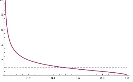
Figure 1. Probability density defined by the two independent solutions for ˆµ= 0.
particle number in the Fock space. For functions σ that just depend one coordinate
p=πii, the normalisability condition reduces to
Z d~π
√
1−~π2 |σ(πij)| 2 = 2π
1 Z
0
dp √p √
1−p|σ(p)|
2 <∞. (47)
With respect to this measure, the general solutions (43) are always normalisable, for
any value of ˆµ. They are analytical solutions to the effective quantum cosmology model
that correspond to homogeneous, isotropic universes, which in general do not display
any form of semiclassical behaviour. Generic solutions, in particular all solutions if ˆµ
is not of the form ˆµ = 2N(N + 1), diverge as p → 0, as does the probability density
∗ √p
√
1−p|σ(p)|
2. For the first branch of solutions, there can also be a divergence in
√
p
√
1−p|σ(p)|2 asp→1, but for the second branch the probability density remains finite.
The detailed shape of these solutions determines whether they describe condensates
of tetrahedra satisfying with high probability p≪ 1, i.e. the assumption of very small
curvature, relative to the scale of the tetrahedra, that was made in the analysis of [14].
Let us look at some specific choices for ˆµ. First, we take ˆµ to be non-negative. If
ˆ
µ = 2N(N + 1) for some non-negative integer N, the first branch of solutions simply
becomes a polynomial in p. In the simplest case where ˆµ = 0, this is just a constant
(Fig. 1; in all of these plots the first branch is plotted in dashed blue while the second
branch is thick red). The second branch is clearly peaked near p= 0.
For ˆµ = 12, the respective probability densities are shown in Fig. 2. While they
are maximal nearp= 1 and p= 0, respectively, the distributions they define are broad,
and not clearly compatible with assuming that most tetrahedra should have p≪1.
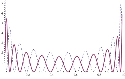
Oscillating solutions arise only for large enough positive values for ˆµ. We show the
two probability densities for ˆµ = 220 in Fig. 3. Both define rather broad probability
distributions, incompatible with assuming p ≪ 1. This is due to the measure in (47),
as |σ(p)|2 alone is peaked near p = 0 in both cases; conclusions drawn from the WKB
0.2 0.4 0.6 0.8 1.0 2
[image:19.612.186.401.93.229.2]4 6 8 10
Figure 2. Probability density defined by the two independent solutions, ˆµ= 12.
0.2 0.4 0.6 0.8 1.0 1
2 3 4 5 6 7
Figure 3. Probability density defined by the two independent solutions, ˆµ= 220.
limit can be modified when one uses the proper type of inner product.
For negative values of ˆµ, both branches of solutions are strongly peaked on values
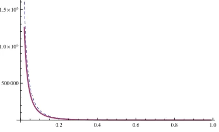
close to zero. We give the probability densities for ˆµ =−4 in Fig. 4 and for ˆµ= −12
in Fig. 5. For ˆµ < 0, the model can be claimed to be predict a condensate of almost
flat tetrahedra. Ultimately, the fundamental GFT model determines whether positive
or negative ˆµ, or ˆµ≫1, should be considered (in many examples such as [28], ˆµ <0).
By redoing the WKB analysis of [13, 14] and by analytical computation of simple solutions of the effective quantum cosmological dynamics, we have shown that the WKB argument which was seemingly in contradiction with having near-flat tetrahedra cannot be trusted. The solutions we found either do not oscillate rapidly or do not agree with
the WKB result, due to the choice of inner product. The solutions for ˆµ > 0 define
broad distributions while for ˆµ < 0 they are peaked nearp= 0. They are normalisable
for any value of ˆµif one takes the wavefunctionσas defining a single-particle condensate
[image:19.612.184.402.279.416.2]0.2 0.4 0.6 0.8 1.0 500
[image:20.612.186.410.93.228.2]1000 1500 2000 2500 3000 3500
Figure 4. Probability density defined by the two independent solutions, ˆµ=−4.
0.2 0.4 0.6 0.8 1.0 500 000
1.0´106
1.5´106
Figure 5. Probability density defined by the two independent solutions, ˆµ=−12.
5. Discussion
Condensate states in group field theory can be used to derive effective quantum cosmology models directly from a proposal for the dynamics of a quantum theory
of discrete geometries. We have illustrated the interpretation of the configuration
space of gauge-invariant geometric data of a tetrahedron, the domain of the condensate wavefunction, as a minisuperspace of spatially homogeneous 3-metrics.
The approach taken here is very different from the more conventional one of quantising only classical degrees of freedom that remain after imposing a symmetry. It makes assumptions about the approximate form of a fully dynamical quantum gravity state, similar to the assumptions one makes when treating interacting quantum systems in condensed matter physics. The validity of these assumptions can be verified; for instance, one can compute fluctuations around the mean field given by the condensate
wavefunctionσ(gI) and see whether they remain small. From the classical interpretation
[image:20.612.187.405.272.403.2]was our main motivation for revisiting the model of [13, 14]. We found that a more consistently derived WKB approximation has a second solution corresponding to flat
universes. Then, rather than assuming semiclassical properties for the condensate
wavefunction, we gave simple isotropic solutions to the full quantum cosmology equation.
These solutions depend on the ‘mass parameter’ µ. For negative µ, they violate the
assumptions of the WKB approximation, but are peaked on small curvature p ≪ 1
and thus consistent with the expectations of the classical picture, as well as with the
Friedmann equationp≈0. For positiveµstates show a wider distribution of curvature.
The effective Friedmann equation (37), as discussed in [13, 14], came out of the WKB approximation of (10) with (30). Once it is accepted that a WKB-type condensate wavefunction may not give a physically relevant approximation to the dynamics, one might ask whether (30) still corresponds to an interesting model of quantum cosmology. The explicit examples given in the paper show that this depends strongly on the value
of the ‘mass parameter’ µ in the fundamental theory; this parameter dropped out in
the WKB limit. For negative µ solutions are strongly peaked near p = 0, and (30)
implements the Friedmann equation p = 0 describing a pure vacuum, spatially flat
universe. In any case, (30) remains a useful example to consider, because it is simple enough for explicit solutions to be constructed, so that the physical interpretation of GFT condensates and their cosmology can be discussed. Further work will be required to conclusively answer whether the model can reproduce some features of general relativity. In the reduction to isotropic states, the model we have studied is fully constrained: there is only one degree of freedom (essentially given by the scale factor) and one constraint. One could add anisotropies or include matter degrees of freedom into the model. For instance, a massless scalar field can be introduced [14] by taking
ˆ
K=
4 X
I=1
∆gI +τ
∂2
∂φ2 +µ (48)
for an extended GFT model with a field onG4×RwhereRparametrises the scalar field.
Adopting this prescription and decomposing σ(p, φ) = P
ωσω(p)eiωφ, general isotropic
solutions would be superpositions of the solutions given above with ˆµ= 1
4(µ−τ ω
2), and
one could try to construct wavepackets similar to [31]. Requiring these to be composed
out of rapidly oscillating modes would require choosing τ < 0 and/or a restriction on
the values of ω, depending on the value of µ. The physical meaning of these conditions
and of the choice (48) from the viewpoint of quantum gravity is however rather unclear.
We conclude that the criterion of semiclassicality for condensate states describing
quantum cosmology has to be phrased more carefully to justify results such as an effective Friedmann equation (37) that can support the potential usefulness of the choice (30) for quantum cosmology. It is only for large-scale observables, such as the total volume (of the universe), that semiclassical behaviour is required. The condensate wavefunction itself captures the properties of what presumably describes a highly quantum-mechanical many-particle state of Planck-scale objects. It carries much more
between different quanta or about the scaling of geometric observables with the particle number. Using this information will be necessary for adding inhomogeneities [14], and for potentially making contact with CMB observations. All of this motivates further systematic studies of the quantum cosmology of (loop) quantum gravity condensates.
Acknowledgements
I thank Daniele Oriti and the referees for helpful and valuable comments on the manuscript. Research at Perimeter Institute is supported by the Government of Canada through Industry Canada and by the Province of Ontario through the Ministry of Research & Innovation.
References
[1] Oriti D 2009Approaches to Quantum Gravity: Toward a New Understanding of Space, Time and Matter(Cambridge: Cambridge University Press)
[2] Amelino-Camelia G 2013 Quantum-Spacetime PhenomenologyLiving Rev. Rel.165 (Website) [3] Ade P A Ret al.2013 Planck 2013 results. XVI. Cosmological parametersarXiv:1303.5076 [4] Ade P A R et al. 2014 BICEP2 I: Detection Of B-mode Polarization at Degree Angular Scales
Phys. Rev. Lett.112241101arXiv:1403.3985
[5] Borde A, Guth A H and Vilenkin A 2003 Inflationary Spacetimes Are Incomplete in Past Directions
Phys. Rev. Lett.90151301gr-qc/0110012
[6] Bousso R, Freivogel B, Leichenauer S, and Rosenhaus V 2011 Eternal inflation predicts that time will endPhys. Rev. D83023525arXiv:1009.4698
[7] Lyth D H 1997 What Would We Learn by Detecting a Gravitational Wave Signal in the Cosmic Microwave Background Anisotropy? Phys. Rev. Lett.781861–1863hep-ph/9606387
[8] Wiltshire D L 1996 An introduction to quantum cosmology Cosmology: The Physics of the Universeed B Robsonet al(Singapore: World Scientific) gr-qc/0101003
[9] Kiefer C and Kr¨amer M 2012 Quantum Gravitational Contributions to the Cosmic Microwave Background Anisotropy SpectrumPhys. Rev. Lett.108021301arXiv:1103.4967
[10] Thiemann T 2008 Modern Canonical Quantum General Relativity (Cambridge: Cambridge University Press)
[11] Bojowald M 2008 Loop quantum cosmologyLiving Rev. Rel.114 (Website)
[12] Agullo I, Ashtekar A and Nelson W 2012 Quantum Gravity Extension of the Inflationary Scenario
Phys. Rev. Lett.109251301arXiv:1209.1609
[13] Gielen S, Oriti D and Sindoni L 2013 Cosmology from Group Field Theory Formalism for Quantum GravityPhys. Rev. Lett.111031301arXiv:1303.3576
[14] Gielen S, Oriti D and Sindoni L 2014 Homogeneous cosmologies as group field theory condensates
JHEP1406013arXiv:1311.1238
[15] Battisti M V, Marciano A and Rovelli C 2010 Triangulated Loop Quantum Cosmology: Bianchi IX and inhomogenous perturbationsPhys. Rev. D81064019arXiv:0911.2653; Bianchi E, Rovelli C and Vidotto F 2010 Towards Spinfoam CosmologyPhys. Rev. D82084035arXiv:1003.3483; Alesci E and Cianfrani F 2013 A new perspective on cosmology in Loop Quantum GravityEPL
104 10001arXiv:1210.4504; Alesci E and Cianfrani F 2013 Quantum-reduced loop gravity: CosmologyPhys. Rev. D87083521arXiv:1301.2245
[16] Oriti D 2013 Group field theory as the 2nd quantization of Loop Quantum Gravity arXiv:1310.7786(revised second version is in preparation)
[18] Baratin A, Girelli F, and Oriti D 2011 Diffeomorphisms in group field theoriesPhys. Rev. D 83 104051arXiv:1101.0590
[19] Dittrich B 2012 From the discrete to the continuous: Towards a cylindrically consistent dynamics
New J. Phys.14123004arXiv:1205.6127
[20] Bojowald M, Chinchilli A L, Dantas C C, Jaffe M, and Simpson D 2012 Non-linear (loop) quantum cosmologyPhys. Rev. D86124027arXiv:1210.8138
[21] Giulini D 2009 The Superspace of Geometrodynamics Gen. Rel. Grav. 41 785–815 arXiv:0902.3923
[22] Perez A 2013 The Spin-Foam Approach to Quantum GravityLiving Rev. Rel.163 (Website) [23] Baratin A and Oriti D 2011 Quantum simplicial geometry in the group field theory formalism:
reconsidering the Barrett–Crane modelNew J. Phys.13125011arXiv:1108.1178
[24] Gielen S and Wise D K 2012 Spontaneously broken Lorentz symmetry for Hamiltonian gravity
Phys. Rev. D 85 104013 arXiv:1111.7195; Wise D K 2012 The geometric role of symmetry breaking in gravityJ. Phys. Conf. Ser.360012017arXiv:1112.2390
[25] Garc´ıa-Compe´an H, Obreg´on O, and Ram´ırez C 2002 Noncommutative Quantum CosmologyPhys. Rev. Lett.88 161301hep-th/0107250
[26] Gibbons G W 2002 The Maximum tension principle in general relativityFound. Phys. 32 1891– 1901hep-th/0210109
[27] Oriti D and Raasakka M 2011 Quantum Mechanics onSO(3) via Non-commutative Dual Variables
Phys. Rev. D84025003arXiv:1103.2098
[28] Ben Geloun J and Bonzom V 2011 Radiative corrections in the Boulatov-Ooguri tensor model: The 2-point functionInt. J. Theor. Phys.502819–2841arXiv:1101.4294
[29] Carrozza S, Oriti D and Rivasseau V 2014 Renormalization of a SU(2) Tensorial Group Field Theory in Three DimensionsCommun. Math. Phys.330581–637arXiv:1303.6772