Low-Complexity Direction-of-Arrival Estimation Based on Wideband Co-Prime Arrays

Wideband Co-Prime Arrays

.

White Rose Research Online URL for this paper:

http://eprints.whiterose.ac.uk/90486/

Version: Accepted Version

Article:

Shen, Q., Liu, W., Cui, W. et al. (3 more authors) (2015) Low-Complexity

Direction-of-Arrival Estimation Based on Wideband Co-Prime Arrays. IEEE/ACM

Transactions on Audio, Speech and Language Processing, 23 (9). 1445 - 1456. ISSN

2329-9290

https://doi.org/10.1109/TASLP.2015.2436214

[email protected] https://eprints.whiterose.ac.uk/

Reuse

Unless indicated otherwise, fulltext items are protected by copyright with all rights reserved. The copyright exception in section 29 of the Copyright, Designs and Patents Act 1988 allows the making of a single copy solely for the purpose of non-commercial research or private study within the limits of fair dealing. The publisher or other rights-holder may allow further reproduction and re-use of this version - refer to the White Rose Research Online record for this item. Where records identify the publisher as the copyright holder, users can verify any specific terms of use on the publisher’s website.

Takedown

If you consider content in White Rose Research Online to be in breach of UK law, please notify us by

Low-Complexity Direction-of-Arrival

Estimation Based on Wideband Co-Prime

Arrays

Qing Shen, Wei Liu,

Senior Member, IEEE,

Wei Cui, Siliang Wu, Yimin D. Zhang,

Senior Member, IEEE,

and Moeness G. Amin,

Fellow, IEEE

Abstract—A class of low-complexity compressive sensing based direction-of-arrival (DOA) estimation methods for wideband co-prime arrays is proposed. It is based on a recently proposed narrowband estimation method, where a virtual array model is generated by directly vectorizing the covariance matrix and then using a sparse signal recovery method to obtain the estimation result. As there are a large number of redundant entries in both the auto-correlation and cross-correlation matrices of the two sub-arrays, they can be combined together to form a model with a significantly reduced dimension, thereby leading to a solution with much lower computational complexity without sacrificing performance. A further reduction in complexity is achieved by removing noise power estimation from the formulation. Then, the two proposed low-complexity methods are extended to the wideband realm utilizing a group sparsity based signal reconstruction method. A particular advantage of group sparsity is that it allows a much larger unit inter-element spacing than the standard co-prime array and therefore leads to further improved performance.

Index Terms—Microphone arrays, direction-of-arrival estima-tion, sparsity, wideband, co-prime.

I. INTRODUCTION

Traditionally, for wideband uniform linear arrays (ULAs), including microphone arrays, the minimum inter-element spac-ing between adjacent sensors is less than λmin/2 to avoid spatial aliasing, whereλminis the minimum wavelength within the frequency band of interest [3]–[5]. This can be problematic when considering arrays with a large aperture size, due to the cost associated with the number of sensors. In the past, sparse arrays have been proposed as a solution [6]–[12], where their non-uniform configuration can avoid grating lobes, while allowing adjacent physical sensor spacings to be greater than

λmin/2.

Recently, a new class of sparse arrays, referred to as co-prime arrays, was proposed [13], [14]. Assume M and N

are co-prime. Then, a co-prime array can be constructed by two sub-arrays, with number of sensors varying based on the values of M and N. A typical co-prime array consists of

The work of Y. D. Zhang and M. G. Amin was supported in part by the Office of Naval Research under Grant N00014-13-1-0061. Part of the work was published in [1] and [2].

Q. Shen is with the School of Information and Electronics, Beijing Institute of Technology, Beijing, 100081, China, and also with the Department of Electronic and Electrical Engineering, University of Sheffield, Sheffield, S1 3JD, UK (e-mail: [email protected]).

W. Liu is with the Department of Electronic and Electrical Engineering, University of Sheffield, Sheffield, S1 3JD, UK (e-mail: [email protected]). W. Cui and S. Wu are both with the School of Information and Elec-tronics, Beijing Institute of Technology, Beijing, 100081, China (e-mail:

{cuiwei,siliangw}@bit.edu.cn).

Y. D. Zhang and M. G. Amin are both with the Center for Advanced Communications, Villanova University, Villanova, PA 19085, USA (e-mail:

{yimin.zhang,moeness.amin}@villanova.edu).

two sub-arrays sharing a sensor at the zeroth position, one with2M sensors and the other with N sensors. The adjacent sensor spacing for the first sub-array is N d, while it is M d

for the second sub-array, where d is the unit inter-element spacing and also the adjacent virtual sensor spacing of the resultant co-prime difference array (as a result, we need to haved≤λ/2, whereλis the operating frequency of the co-prime array). As such, with a total number of 2M +N −1 sensors, the difference co-array of the two sub-arrays can provide more than M N degrees of freedom. The increased degrees of freedom (DOFs) can be exploited for effective direction of arrival (DOA) estimations [14]–[17]. In [14], a virtual array of a larger aperture is generated from the co-prime array by vectorizing the covariance matrix, with equivalent coherent impinging signals. Then, a rank restoring method based upon spatial smoothing is utilized for DOA estimation [18], [19]. Under the condition of imperfect correlation matrix, sparsity-based signal recovery method is applied in [15]. In [17], a sparse signal recovery method based on compressive sensing is used for narrowband DOA estimation, employing a ULA with two co-prime frequencies. The aforementioned methods were all designed for narrowband waveforms.

For wideband DOA estimation, several methods have been proposed, most notably the incoherent signal subspace method [20], the coherent signal subspace method [21], the test of orthogonality of projected subspaces method [22], and the recently proposed approximate maximum likelihood approach [23]. In particular, a series of DOA estimation methods based on the sparse signal recovery approach were developed in [24], [25]. In [26], a subband information fusion method based on the concept of group sparsity is introduced to jointly explore the information in all subbands.

0 M d 2M d (N−1)M d

• • • · · · •

• • • • · · · •

[image:3.612.85.268.59.117.2]

0 N d 2N d (2M −1)N d

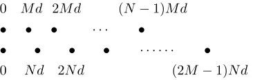
Fig. 1. Structure of a general co-prime array.

provided by all subbands. It is shown that, with a much lower computational complexity, the proposed methods for the single frequency case achieve a very similar performance to the existing one, whereas their respective wideband extensions exhibit a significantly improved performance compared to the narrowband ones.

It is well-known that the resolution of an array improves with an increased aperture size. However, to avoid aliasing, traditionally, a spacing between adjacent sensors of a ULA smaller than λmin/2 is commonly used. An advantage of the proposed group sparsity based methods is that the equivalent spacing d between adjacent virtual sensors of the co-prime array can be increased beyond λmin/2, while still avoiding spatial aliasing in the estimated results. This is because alias-ing locations for different frequencies are different and our group sparsity based methods will force a common sparsity location across all frequencies, corresponding to the true location of the impinging signals. In this respect, we enable the use of a larger inter-element spacing than that associated with the standard co-prime array, leading to a further improved DOA estimation performance.

Our contributions are therefore: 1) Developing the group sparsity-based wideband DOA estimation beyond our prelim-inary results in [1]; 2) Developing low complexity narrowand and wideband DOA estimation using sparse reconstruction by removing the noise term and recognizing the built in redundancies in subarray auto-correlation and cross-correlation lags; 3) Extending the array aperture by permitting a larger sensor spacing than that defined by half of the minimum wavelength.

This paper is organized as follows. The wideband signal model for co-prime arrays is presented in Section II. The proposed low-complexity DOA estimation method is intro-duced in Section III for a single frequency. Their wideband extensions are then given in Section IV-A to Section IV-C, and the co-prime arrays with further improved performance due to an increased spacing is presented in Section IV-D. Simulation results are provided in Section V, and results based on collected acoustic data is presented in Section VI. Conclusions are drawn in Section VII.

II. SIGNALMODEL WITHCO-PRIMEARRAYS

A co-prime array consists of two uniform linear sub-arrays, as shown in Fig. 1, where M < N is assumed. The first sub-array has N sensors with an inter-element spacing of M d, and the second one has 2M sensors separated byN d, where

d≤λmin/2. Note another layout of the co-prime array usesM

sensors for the second sub-array, instead of2M. The proposed methods here are equally applicable to both cases.

The zeroth positions of the two sub-arrays share the same sensor and in total there are 2M +N −1 sensors. Denote the set of sensor positions for the two sub-arrays as S1 and

S2, respectively. The zeroth sensor is removed in S2 for convenience of formulation at a later stage, i.e.,

S1={M nd, 0≤n≤N−1, n∈Z_{} ,}

S2={N md, 1≤m≤2M−1, m∈Z_{} ,} (1)

whereZ_{is the set of all integers.}

Assume that there are K uncorrelated wideband signals

sk(t)with the same bandwidth impinging from incident angles

θk, k= 1,2, . . . , K, respectively, where θk is measured from

the broadside of the array. Then, the signals observed from an element in the two sub-arrays can be expressed as:

x1,n(t) = K

∑

k=1

sk[t−τ1,n(θk)] +n1,n(t),

x2,m(t) = K

∑

k=1

sk[t−τ2,m(θk)] +n2,m(t),

(2)

where 0 ≤ n ≤ N −1 and 1 ≤ m ≤ 2M −1. Take the zeroth position of the co-prime array as the reference. Then,

τ1,n(θk) and τ2,m(θk) represent the time delay of the k-th

impinging signal with the incident angle θk arriving at the

n-th sensor of the first sub-array and them-th sensor of the second sub-array, respectively.n1,n(t)andn2,m(t) are white

noise at the corresponding sensors.With a sampling frequency

fs, the discrete version of the two sets of sub-array signals

can be expressed as

x_{1[i] =}[_{x1,0[i], x1,1[i], . . . , x1,N−1[i]}]T _,

x_{2[i] =}[_{x2,1[i], x2,2[i], . . . , x2,2M−1[i]}]T _,

(3)

where{·}T _{denotes the transpose operation andithe}

discrete-time variable.

Each received sensor signal is divided into non-overlapping groups with lengthL, and anL-point DFT is applied. Then, the l-th frequency bin/subband samples of the p-th group for each sub-array can be grouped into one vector as follows

X_{1[l, p] =}[_{X1,0[l, p], X1,1[l, p], . . . , X1,N} −1[l, p]

]T

,

X_{2[l, p] =}[_{X2,1[l, p], X2,2[l, p], . . . , X2,2M} −1[l, p]

]T

, (4)

where

X1,n[l, p] = L_∑−1

i=0

x1,n[L·(p−1) +i]·e−j

2π Lil,

X2,m[l, p] = L₋1

∑

i=0

x2,m[L·(p−1) +i]·e−j

2π Lil,

(5)

withp= 0,1, . . . , P−1, andl= 0,1, . . . , L−1.

Define Sk[l, p], N1,n[l, p], and N2,m[l, p] as the DFT of

thep-th group discrete-time impinging signalssk[i],

discrete-time noises at sensors of the two sub-arrays n1,n[i] and

n2,m[i], respectively. S[l, p] =

[

S1[l, p], . . . , SK[l, p]

]T

is a column vector holding signals at the l-th frequency bin, and N_{1[l, p] =} [_{N1,0[l, p], . . . , N1,N}

−1[l, p] ]T

[

N2,1[l, p], . . . , N2,2M−1[l, p] ]T

are the corresponding col-umn noise vectors at the two sub-arrays. Then, the output signal model in the DFT domain can be expressed as

X_{1[l, p] =}A_1(l,θ₎S_{[l, p] +}N_{1[l, p],}

X_{2[l, p] =}A_2(l,θ₎S_{[l, p] +}N_{2[l, p],} (6)

where A_1(l,θ_{) = [}a_{1(l, θ1), . . . ,}a_{1(l, θK)] and} A_2(l,θ_{) =}

[a_{2(l, θ1), . . . ,}a_{2(l, θK)]are the steering matrices at frequency}

flcorresponding to thel-th frequency bin. The column vectors

a_{1(l, θk)and}a_{2(l, θk)are the steering vectors at frequencyfl} and angle θk, given as

a_{1(l, θk) =} [

1, e−j2πM d

λl sin(θk)_{, . . . , e}−j2πM(N−1)d λl sin(θk)

]T

,

a_{2(l, θk) =} [

e−j2πN d λl sin(θk)

, . . . , e−j2πN(2M−1)d λl sin(θk)

]T

,

(7)

whereλl=c/flandcis the wave speed. For eachlof interest,

(6) can be considered as a narrowband signal model.

III. SPARSITY-BASEDLOW-COMPLEXITYDOA ESTIMATION FOR ASINGLEFREQUENCY

In this section, we first review the narrowband DOA esti-mation method for co-prime arrays proposed in [16], using the single-frequency model in (6) as an example in Subsec-tion III-A, and then propose our two low-complexity DOA estimation methods in Subsections III-B and III-C.

A. Review of DOA estimation for narrowband co-prime arrays

We consider DOA estimation using the data at the l-th frequency bin. Denote X_{[l, p] =}[XT_{1[l, p],}XT_{2[l, p]}]T_{. Then,} the covariance matrix forX_{[l, p] is}

R_{xx[l] = E}{X_{[l, p]·}XH_{[l, p]}}

=

K

∑

k=1

σ2k[l]a(l, θk)aH(l, θk) +σ2¯n[l]I2M+N₋1,

(8)

where {·}H _{denotes Hermitian transpose, E{·} is the}

ex-pectation operator, a_{(l, θk) =} [aT

1(l, θk),aT2(l, θk)

]T

and I_2M+N

−1 is the (2M+N−1) ×(2M +N−1) identity matrix.σ2

k[l]represents the power of thek-th impinging signal

at thel-th frequency bin, andσ2 ¯

n[l]is the corresponding noise

power.

In practice,R_{xx[l] can be estimated by}

R_xx[l]≈Rb_{xx[l] =} 1

P

P_∑−1

p=0

X_{[l, p]·}XH_{[l, p], (9)}

where P is the number of signal blocks for DFT and we assume that the impinging source signals are wide-sense stationary over this period.

Vectorizing R_{xx[l] yields}

z_{[l] = vec{}R_xx[l]}=Ae_[l]es_{[l] +σ}2

¯

n[l]eI2M+N−1, (10) where Ae_{[l] = [e}a_{(l, θ1), . . . ,e}a_{(l, θK)] with e}a_{(l, θk) =} a∗_{(l, θk)⊗}a_{(l, θk)(⊗is the Kronecker product and{·}}∗ de-notes the conjugate operation), andes_{[l] =}[_σ2

1[l], . . . , σK2[l]

]T

.

eI_2M+N

−1is a(2M +N−1)

2

×1column vector obtained by vectorizingI_2M+N

−1.

Equation (10) characterises a virtual array with a higher number of DOFs, where Ae_{[l] represents its steering matrix} andes_{[l]represents its equivalent impinging signal vector. Note} that the increased DOFs are only available in the signal and noise power domain, which enable the DOA estimation of the signals, but cannot be used to recover their waveforms. Ae_[l] contains virtual sensor positions distributed in the set of cross differences

{

±(N m−M n)·d,0≤n≤N−1∩1≤m≤2M −1}

and the two sets of self differences

{(N m1−N m2)·d,1≤m1≤2M −1,1≤m2≤2M −1},

{(M n1−M n2)·d,0≤n1≤N−1,0≤n2≤N−1}.

Moreover, (10) can be modified into

z_{[l] =}Ae_[l]es_{[l] +σ}2_¯n[l]eI_2M+N

−1=Ae◦[l]es◦[l], (11) whereAe◦_{[l] =}

[ e

A_[l],eI_2M+N−1 ]

andes◦_{[l] =}[_esT_{[l], σn}2_¯[l]]T_. For the l-th frequency bin, with a search grid of Kg

potential incident angles θg,1, . . . , θg,Kg, the steering matrix

is generated byAe_{g[l] =}[_ea_{(l, θg,1), . . . ,e}a_{(l, θg,K}

g)

]

. Here we use the subscript{·}gto describe matrices, vectors or elements

related to the generated search grid. Construct a column vector es_{g[l]consisting ofKg elements, each representing a potential} source signal at the corresponding incident angle. Denote

e A◦

g[l] =

[ e

A_g[l],eI_2M+N −1

]

, es◦ g[l] =

[

es_{g[l], σn¯}2_[l]]T_{. (12)}

The last elementσ2 ¯

n[l]ines◦g[l]can also be considered as a variable because the noise power is unknown. All the elements ines◦_{[l]are powers, and therefore positive real numbers. The} method proposed in [16] can be applied to a single frequency in the wideband case directly with the following formulation

min es◦

g[l]

1

subject to

z_[l]−Ae◦ g[l]es

◦ g[l]

2≤ε ,

e

s◦

g,kg[l]≥0, 0≤kg≤Kg,

(13)

whereεis the allowable error bound,∥·∥₁is thel1 norm and ∥·∥₂ the l2 norm. se◦

g,kg[l] represents the kg-th entry in the

column vectores◦ g[l].

B. Low-complexity DOA estimation for a single frequency

We first add the received signal of the zeroth sensor into the signal vector of the second sub-array. Then (4) changes to

X_{1[l, p] =}[_{X1,0[l, p], . . . , X1,N} −1[l, p]

]T

,

X_{2[l, p] =}[_{X2,0[l, p], . . . , X2,2M} −1[l, p]

]T

, (14)

where X2,0[l, p] = X1,0[l, p], and the steering vectors

de-scribed in (7) become

a_{1(l, θk) =} [

1, e−j2πM d

λl sin(θk)

, . . . , e−j2πM(N−1)d λl sin(θk)

]T

,

a_{2(l, θk) =} [

1, e−j2πN d_λl sin(θk)_{, . . . , e}−j2πN(2_λlM−1)dsin(θk)

]T

.

Then, the auto-correlation matrices of the signal vectors observed in the two sub-arrays can be obtained as

R_{11[l] = E}{X_{1[l, p]·}XH

1[l, p]

}

=

K

∑

k=1

σk2[l]a1[l, θk]a1H[l, θk] +σn2¯[l]IN ,

(16)

R_{22[l] = E}

{

X_{2[l, p]·}XH_{2[l, p]} }

=

K

∑

k=1

σk2[l]a2[l, θk]aH2[l, θk] +σn2¯[l]I2M ,

(17)

whereI_{N and}I_{2M are identity matrices with size ofN×N} and2M×2M, respectively. Note here thatR_11[l]andR_22[l] are both Hermitian and Toeplitz.

We can also obtain the cross-correlation matrices of the two sub-arrays, given by

R_{12[l] = E}

{

X_{1[l, p]·}XH_{2 [l, p]} }

=

K

∑

k=1 σ2

k[l]a1[l, θk]aH2[l, θk] +σn2¯[l]WN,2M ,

(18)

R_{21[l] = E}{X_{2[l, p]·}XH

1 [l, p]

}

=

K

∑

k=1

σ2k[l]a2[l, θk]aH1[l, θk] +σn2¯[l]W2M,N ,

(19)

whereW_{N,2M has a size ofN×2M and}W_{2M,N has a size} of 2M ×N, both being all zeroes except for a value of 1 at the (0,0)th entry. We haveR_{12[l] =}RH_21[l].

For0≤n≤N−1 and0≤m≤2M−1, the set of cross difference b=N m−M ncan reach any integer in the range of0toM N [13], [14]. The cross difference sets ofb=N m−

M nand−b=−N m+M nalso contain all the lags included in self difference sets provided by R_{11 and} R_{22 [27]. The} redundant lags can be combined together. Furthermore, the information contained in R_{21[l]is the same as that in} R_12[l]. Therefore, the virtual array generated fromR_{12[l]contains all} the degrees of freedom. In practice,R_12[l],R_{11[l], and}R_22[l] can be replaced by their finite-sample estimatesRb_12[l],Rb_21[l],

b

R_{11[l], and}Rb_{22[l], respectively.} Considering Rb_{11[l] =} RbH

11[l], Rb22[l] = RbH22[l], and

b

R_{12[l] =} RbH

21[l], the complex conjugate part in matrices

b

R_11[l], Rb_{22[l], and the entire matrix} Rb_{21[l] can be removed} in virtual array generation for complexity reduction. A more accurate estimation of the virtual array model can be obtained by averaging all the entries with the same lag in auto-correlation matrices. DenoteR_{c[l]as the new cross-correlation} matrix at the l-th frequency bin. Then, the entry in the n-th

row and them-th column of R_{c[l]is expressed as}

Rn,mc [l] =

                                  

N∑−1

ˆ

n=0

b

R11ˆn,nˆ[l] + 2M∑−1

ˆ

m=1

b

Rm,22ˆ mˆ[l]

2M+N−1 , n, m= 0,

2M∑−1

ˆ

m=m

b

Rmˆ−m,mˆ 22 [l]

2M−m , n= 0, m̸= 0,

N_∑−1

ˆ

n=n

b

Rn,ˆnˆ−n

11 [l]

N−n , n̸= 0, m= 0,

b

Rn,m12 [l], others,

(20) where the superscripts are the corresponding row and column indexes.

In (20), an accurate estimation of R_{12 is obtained by} removing duplicate entries and combining redundant entries inR_{11 and}R_{22. Furthermore, redundant entries in}R_{12 can} also be combined for further complexity reduction.

Then-th row andm-th column entry in R_{12 is}

R12n,m[l] =

      

K

∑

k=1 σ2

k[l]e−

j2π(nM−mN)d

λl sin(θk)_+σ2 ¯

n[l], m=n= 0, K

∑

k=1 σ2

k[l]e−

j2π(nM−mN)d λl sin(θk)_,

others.

(21)

Signal powersσ2

k[l], k= 1,2,· · · , K,and noise powerσn2¯[l]

are all positive real numbers. Considering indexes of(n1, m1) and(n2, m2),Rn1,m1

12 [l]andR

n2,m2

12 [l]are complex conjugate

when the indexes satisfy the following relationship

n1M −m1N =−(n2M−m2N),

which can be modified as

(n1+n2)M = (m1+m2)N , (22)

where0≤n1≤N−1,0≤n2≤N−1,0≤m1≤2M−1, and0≤m2≤2M−1. Then, the only necessary and sufficient condition of (22) is

n1+n2=N∩m1+m2=M . (23)

Thus, we can obtain the following relationship in matrixR₁₂

Rn1,m1

12 [l] =

{

Rn2,m2

12 [l]

}∗

={RN−n1,M−m1

12 [l]

}∗

, (24)

updated to

¯

Rn,mc [l] =

                                                        

N∑−1

ˆ

n=0

b

Rn,₁₁ˆnˆ[l] +

2M∑−1

ˆ

m=1

b

R₂₂m,ˆ mˆ[l]

2M+N−1 , n, m= 0,

2M_∑−1

ˆ

m=m

b

Rmˆ−m,mˆ

22 [l]

2M−m , n= 0, m̸= 0,

N∑−1

ˆ

n=n

b

Rn,ˆnˆ−n

11 [l] +{ bR

N−n,M−m

12

}∗

N−n+ 1 , n̸= 0, m= 0, { N_∑−1

ˆ

n=N₋n

b

Rn,ˆnˆ−N+n

11 [l]

}∗

+Rbn,m12

n+ 1 , n̸= 0, m=M, b

Rn,m₁₂ +{ bRN−n,M−m

12

}∗

2 , n̸= 0,1≤m < M,

b

Rn,m12 [l], others,

(25)

whereR¯n,m

c [l] is then-th row and them-th column entry in

the updated smoothed cross-correlation matrix Rn,m c [l]. Matrix R_{c[l] corresponds to the cross difference co-array} −b=M n−N m, with the ability of reaching all the integers in the range of −M N to 0, where 0 ≤ n ≤ N −1 and 0 ≤ m≤2M −1. According to (21) and (25), the positive lags in the cross difference co-array −b =M n−N mhave been combined and can be removed when vectorizing R_c[l], and the number of positive lags is (N−1)(M+1)

2 .

¯

z_{c[l]is the vector obtained by vectorizing}R_{c[l], i.e.}

¯z_{c[l] = vec}{R_c[l]}

=Ae_c[l]es_{[l] +σ}2

¯

n[l]weN,2M =Ae◦c[l]es

◦_[l], (26)

where Ae_{c[l] =} [_ea_{c[l, θ1], . . . ,e}a_{c[l, θK]}] _{with e}a_{c[l, θk] =} a∗

2[l, θk]⊗a1[l, θk], andes[l] =

[

σ2

1[l], . . . , σK2[l]

]T

.we_{N,2M is} a2M N×1column vector obtained by vectorizing the matrix W_N,2M.Ae◦

c[l]andes◦[l] are given as

e A◦

c[l] =

[ e

A_c[l],w_eN,2M ]

, es◦_{[l] =}[_esT_{[l], σ}2 ¯

n[l]

]T

. (27)

With the same search grid of Kg potential angles

θg,1, . . . , θg,Kg as used earlier, the steering matrix is generated

by Ae_{cg[l] =} [_ea_{c[l, θg,1], . . . ,e}a_{c[l, θg,K}

g]

]

. Construct a Kg

-element column vectores_{g[l], with each element representing} a potential source at the corresponding incident angle. Denote

e A◦

cg[l] =

[ e

A_cg[l],Wf_N,2M ]

, es◦ g[l] =

[ e sT

g[l], σ

2 ¯

n[l]

]T

. (28)

We use nc, 0 ≤ nc ≤ 2M N −1, to denote the row index

of the column vector¯z_{c[l], the matrix} Ae_{c[l] in (26), and the} matrixAe_{cg[l]in (28). Then, each entry of}¯z_{c[l]is expressed as} ¯

znc[l]. Row vectorsaec,nc[l]andeacg,nc[l]are used to represent

the nc-th row of the matrices Aec[l]and Aecg[l], respectively. Denote nc,n0 ∈Φ, n0= 0,1,· · · , N0−1, as the row indexes

corresponding to all the negative lags, where N0 = 2M N−

(N₋1)(M+1)

2 is the number of indexes setΦ ={N m+n,0≤

n≤N−1∩0≤m≤2M −1∩M n−N m≤0}. Keeping all the row indexesnc,n0, we obtain a virtual array model as

ˇz_{c[l] = ˇ}A◦

c[l]es

◦_{[l], (29)}

where ˇz_{c[l] =} [_z¯n

c,0[l],· · ·,z¯nc,N0−1[l]

]T

and Aˇ◦ c[l] =

[ e aT

c,nc,0[l],· · ·,ea

T

c,nc,N0−1[l]

]T

.

Then the proposed low-complexity DOA estimation method can be expressed as

min es◦

g[l]

1

subject to ˇz_c[l]−Aˇ◦ cg[l]es

◦ g[l]

2≤ε ,

e

s◦

g,kg[l]≥0, 0≤kg≤Kg,

(30)

whereAˇ◦ cg[l] =

[ e aT

cg,nc,0[l],· · · ,ea

T

cg,nc,N0−1[l]

]T

, andseg,kg[l]

is the kg-th entry of column vectoresg[l].

In (13) and (30), the first Kg elements of es◦g[l] give the corresponding DOA estimation results over Kg search grids.

Compared with (13), there is a significant reduction in the number of entries in the optimization problem (30) due to the combination of redundant entries, leading to reduction in com-putational complexity using various optimisation toolboxes.

C. Further reduction by removing noise power estimation

In (26), we_{N,2M is an all-zero column vector except for} the zeroth entry. Only the zeroth element in ˇz_{c[l] related} to the zero lag is influenced by noise power σ2

¯

n[l], and the

estimation of noise power takes up one DOF. As a result, we can remove the zero lag part to avoid estimating σ2

¯

n[l]

in (30). In so doing, the range of difference co-array lags in R_{c[l] from −M N to −1 with M N DOFs can still be} provided by the co-prime array, with the new set of available DOFs fully dedicated to DOA estimation. Further reduction in computational complexity is achieved due to the reduction in the number of parameters to be estimated and the number of entries.

We use n0, 0 ≤ n0 ≤ N0 −1, to be the row index of ˇ

z_c[l], Aˇ_{c[l] in (29), and} Aˇ_{cg[l] in (30). Then, each entry} of ˇz_{c[l] is expressed as zˇc,n}

0[l]. Row vectors aˇcr,n0[l] and

ˇ a_cg,n

0[l] are used to represent the n0-th row of Aˇc[l] and

ˇ

A_{cg[l], respectively. Removing the first row withn0= 0, we} obtain a virtual array model

z_{s[l] =}Ae_s[l]es_[l], (31)

where z_{s[l] =} [_{zˇc,1[l],· · ·,zˇc,N}

0−1[l] ]T

, and Ae_{s[l] =} [

ˇ aT

cr,1[l],· · · ,aˇTcr,N0−1[l] ]T

.

Then, the modified low-complexity DOA estimation method for a single frequency at the l-th frequency bin can be expressed as

min ∥es_g[l]∥

1

subject to

z_s[l]−Ae_sg[l]es_g[l]

2≤ε

e

sg,kg[l]≥0, 0≤kg≤Kg−1,

(32)

where Ae_{sg[l] =} [a_ˇT

cg,1[l],· · · ,ˇa T

cg,N0−1[l] ]T

, and esg,kg[l] is

The problems in (13), (30), and (32) can be solved using CVX, a software package for specifying and solving convex problems [28], [29].

IV. WIDEBANDDOA ESTIMATIONMETHODBASED ON

GROUPSPARSITY FORCO-PRIMEARRAYS

For wideband signals transformed into multiple frequency bins as described in Section II, we could apply the algorithm in (13), (30), and (32) to the frequency range of interest one by one and then average the results to give the final estimation. A more effective approach that achieves a higher accuracy, however, is to jointly estimate the DOA of the impinging signals across the entire frequency range of interest simultaneously based on the group sparsity concept, i.e., the DOA results corresponding to different frequencies share the same spatial support, although they may have varying power values. Assume that the frequency range or bandwidth of interest covers Q frequency bins in the DFT domain, where theQ≤Lfrequency bins may or may not be adjacent to each other. For each frequency binlq ∈Φl,0≤q≤Q−1, where

Φlis the set ofQfrequency bin indexes, the same search grid

of Kg potential incident angles are used to generate all the

matrices needed as described for each method.

A. Wideband extension 1 based on existing DOA estimation method

First, we construct two matrices: a block diagonal matrix e

B◦

g usingAe◦g[lq], expressed as

e B◦

g= blkdiag

{ e A◦

g[l0],Ae ◦

g[l1], . . . ,Ae ◦ g[lQ−1]

}

(33)

and a (Kg+ 1)×Qmatrix Rg◦ usinges◦g[lq]with

R◦ g=

[ e s◦

g[l0],es ◦

g[l1], . . . ,es ◦ g[lQ−1]

]

. (34)

Then, we obtain the following virtual array model

e z₌Be◦

ger ◦

g, (35)

where ez₌[zT_{[l0], . . . ,z}T_[l Q₋1]

]T

ander◦

g = vec

( R◦

g

) is a (Kg+ 1)·Q×1 column vector by vectorizingR◦g.

We use the row vectorr◦

g,kg,0≤k0≤Kg, to represent the

k0-th row of the matrixR◦

g. Then, we form a new(Kg+1)×1 vector ˆr◦

g based on thel2 norm of r◦g,k0,0≤k0≤Kg

ˆ r◦

g=

[ r◦

g,0

2, . . . ,

r◦

g,Kg

2

]T

. (36)

Finally, our group-sparsity based wideband DOA estimation method is formulated as follows

min

˜r◦

g

ˆr◦

g 1 subject to ez₋Be◦

ger ◦ g

2≤ε ,

e

r◦

g,kg ≥0, 0≤kg≤(Kg+ 1)·Q−1,

(37)

wherer_e◦

g,kg represents thekg-th element of the column vector

e r◦

g, and the nonzero entries in the first Kg elements of the column vector ˆr◦

g are the corresponding wideband DOA estimation results over the Kg search grids.

B. Wideband extension 2 based on proposed low-complexity DOA estimation method

The proposed low-complexity wideband virtual array model extended from narrowband DOA estimation method (30) can be shown as

ˇ z◦

c= ˇB ◦ cger

◦

g, (38)

whereˇz◦ c=

[ zT

c[l0], . . . ,z T c[lQ−1]

]T

,er◦

g= vec

( R◦

g

)

, and the block diagonal matrixBˇ◦

cg given by

ˇ B◦

cg= blkdiag

{_ˇ A◦

cg[l0],Aˇ ◦

cg[l1], . . . ,Aˇ ◦ cg[lQ−1]

}

. (39)

Then, the proposed low-complexity wideband DOA estimation method is formulated as

min

˜

r◦

g

ˆr◦

g

1

subject to ˇz◦ c−Bˇ

◦ cger

◦ g

2≤ε ,

e

r◦

g,kg ≥0, 0≤kg≤(Kg+ 1)·Q−1,

(40)

C. Wideband extension 3 based on further complexity reduc-tion DOA estimareduc-tion method

Two matrices, i.e., block diagonal matrixBe_{sg andKg×Q} matrix R_{g, are constructed using} Ae_{sg[lq] ande}s_g[lq] respec-tively, given by

e

B_{sg= blkdiag}{Ae_sg[l0],Ae_{sg[l1], . . . ,}Ae_sg[lQ

−1] }

,

R_g=[_es_g[l0],es_{g[l1], . . . ,e}s_g[lQ −1]

]

. (41)

Then, the further improved wideband virtual array model is given by

e

z_s=Be_sger_g, (42)

whereez_{s =}[zT

s[l0], . . . ,z T s[lQ−1]

]T

ander_{g = vec (}R_{g)is a}

Kg·Q×1 column vector by vectorizingRg.

Row vector r_{g,k0, 0 ≤k0 ≤Kg−1 is used to represent} thek0-th row ofR_{g. Then, we form a newKg×1 vectorˆ}r_g based on thel2 norm of r_g,k

0,0≤k0≤Kg−1, as

ˆr_g=[r_g,0

2,

r_g,1

2, . . . ,

r_g,K

g−1

2

]T

. (43)

Finally, the modified wideband DOA estimation method based on group sparsity is formulated as follows

min

˜

rg

∥ˆr_g∥

1

subject to

ez_s−Be_sger_g

2≤ε ,

e

rg,kg ≥0, 0≤kg≤Kg·Q−1,

(44)

whereerg,kg represents thekg-th element of the column vector

er_{g, and the nonzero entries in theKg elements of the column} vector ˆr_{g are the corresponding wideband DOA estimation} results over theKg search grids.

D. Performance improvement with large unit spacing

The resolution of an array will improve with an increased aperture size. For existing DOA estimation methods for both narrowband signals and wideband signals, an equivalent unit spacing satisfying d ≤ λmin/2 is normally chosen to avoid spatial aliasing. An advantage of our proposed group sparsity based methods is that we can increase the spacing d to be larger than λmin/2, while still avoiding spatial aliasing. This is because aliasing locations for different frequencies are different and the proposed group sparsity based methods will force a common sparsity location across all frequencies, corresponding to the true location of the impinging signals. Thus, the proposed methods allow a larger spacing than the standard co-prime array, leading to a larger virtual array aperture, and therefore more accurate estimation results can be obtained. However, we can expect that when d is larger than some threshold value, the DOA estimation results will degrade, as will be shown in our simulations part. When

d =λmax/2, where the largest virtual array aperture can be achieved under the condition of no spatial aliasing only for the minimum frequency of interest, we can still perform effective DOA estimation.

V. SIMULATIONRESULTS

Consider a co-prime array with M = 3 andN = 5. With

fs twice the highest frequency of interest, the normalized

frequencies of the impinging signals cover the range from0.5π

to π, and the unit spacing d =λmin/2 withλmin = 2c/fs.

As an example, for a microphone array, this is equivalent to a frequency band from 5 kHz to 10 kHz with a sampling frequency of 20 kHz andλmin = 3.4 cm at a speed of 340 m/s.

The number of signal samples in the time domain at each sensor is128000, and DFT ofL= 64points is applied. Then, the number of data blocks used for estimatingR_xx[l],R_11[l], R_22[l],R_{12[l], and}R_{21[l]at each frequency bin isP = 2000.} There are 15 uncorrelated wideband signals impinging on the array, with incident angles uniformly distributed between −60◦ _and60◦_{. A search grid ofKg= 3601angles is formed} within the full angle range with a step size of 0.05◦_{. The} normalized frequency range of impinging signals covers the frequency bin setΦl={17,18,· · · ,31} withQ= 15.

A. Data Storage Analysis and Computation Time Comparison

First, the number of entries in the vectors/matrices involved is shown in Table I for the three narrowband DOA estimation methods and their wideband extensions. Fewer entries lead to less multiplicative and additive operations in the corresponding formulations, which is then translated into a lower compu-tational complexity. For the underlying example, the exact number of entries is shown in Table II. We see that the existing method in (13) has the largest number of entries among all narrowband methods, while its wideband extension (37) has the largest number of entries among all wideband ones. The computation time using the CVX package, calculated by the MATLAB profiler under the environment of Intel CPU I5-3470 with a clock speed of 3.20GHz and 8GB RAM, is also listed

in Table II. It is clear that the existing method has the longest processing time among all the three narrowband methods, with the one in (32) being the shortest. Their wideband extensions keep the same features.

B. Low-complexity DOA estimation results

For the first set of simulations, the input SNR is0 dB and the allowable error boundε is chosen to give the best result for each method through trial-and-error in every experiment1_.

Specifically, it is set to be 10 for the existing narrowband method in (13), 5 for our proposed low-complexity method in (30), and 4 for our modified method in (32). For the wideband case, 65,25, and 13were chosen as the allowable error bound ε, respectively. The much larger value for ε in the wideband case is due to the norm operation based on

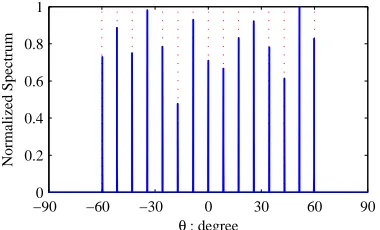
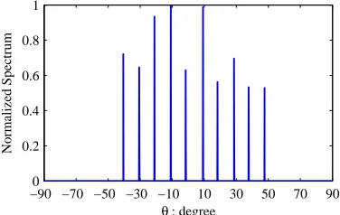
Q= 15frequencies instead of one single frequency. The DOA estimation results for the single frequency (l= 31) are shown in Fig. 2, and the wideband results are shown in Fig. 3, where the dotted lines in the figures represent the actual incident angles of the impinging signals, while the solid lines represent the estimation results. It is clear that all the sources have been distinguished successfully by all the studied methods.

To compare the estimation accuracy with respect to a varied input SNR, the root mean square error (RMSE) results are shown in Fig. 4, where each point is based on an average of the results obtained by 500 simulation runs. Clearly, their narrowband performances are nearly the same for most of the cases, and their wideband extensions share a similar perfor-mance with extensions 2 and 3 being slightly more accurate. Furthermore, these proposed wideband extensions consistently outperform the narrowband ones by a large margin.

Finally, in this part, we give an example where the nar-rowband method clearly fails while the proposed wideband method can still provide a good result. The setting is the same as before except that now there are21sources uniformly distributed between−60◦_and60◦_{. Due to the increased signal} number and reduced separation between DOAs of adjacent signals, the estimation task is much tougher than the previ-ous settings and therefore can show the difference of their performances more effectively. The results of the modified low-complexity method for the single frequency case and its wideband extension are shown in Fig. 5, which again verifies the superior performance of the wideband method.

C. Results with large unit spacing co-prime arrays

Now we increase the unit spacing d to be larger than

λmin/2, with d= df·λmin/2 = df·c/fs, and examine its

effect on the estimation results. To depict the change of the estimation results due to a change ofdf more clearly, a search

grid ofKg= 18001incident angles is formed within the full

angle range with a smaller step size of0.01◦_{. Other parameters}

TABLE I

NUMBER OFENTRIES INVECTORS/MATRICES

Vector / Matrix Methods for a Single Frequency

Existing (13) Proposed (30) Modified (32)

es◦

g[l]/es◦g[l]/esg[l] Kg+ 1 Kg+ 1 Kg

z_[l]/ˇz

c[l]/zs[l] (2M+N−1)2 3

M N−N+M+1

2 3

M N−N+M−1 2 e

A◦

g[l]/Aˇ

◦

cg[l]/Aesg[l] (2M+N−1)2(Kg+ 1) (3

M N−N+M+1)(Kg+1)

2

(3M N−N+M−1)Kg

2

Vector / Matrix Wideband DOA Estimation Methods

Extension 1 (37) Extension 2 (40) Extension 3 (44)

er◦

g/er◦g /erg (Kg+ 1)Q (Kg+ 1)Q Kg·Q

ez_/ˇz◦

c/ezs (2M+N−1)2·Q

(3M N−N+M+1)Q

2

(3M N−N+M−1)Q

2 e

B◦

g/Bˇ◦cg/Besg (2M+N−1)2(Kg+1)Q2

(3M N−N+M+1)(Kg+1)Q2

2

(3M N−N+M−1)KgQ2

2

TABLE II

NUMBER OFENTRIES INVECTORS/MATRICES ANDCOMPUTATIONTIME FOR THEEXAMPLE

Vector / Matrix Methods for a Single Frequency

Existing (13) Proposed (30) Modified (32)

es◦

g[l]/es

◦

g[l]/esg[l] 3602 3602 3601

z_[l]/ˇz

c[l]/zs[l] 100 22 21

e A◦

g[l]/Aˇ

◦

cg[l]/Aesg[l] 360200 79244 75621

Computation Time 16.426s 4.587s 4.072s

Vector / Matrix Wideband DOA Estimation Methods

Extension 1 (37) Extension 2 (40) Extension 3 (44)

er◦

g/er◦g /erg 54030 54030 54015

ez_/ˇz◦

c/ezs 1500 330 315

e B◦

g/Bˇ

◦

cg/Besg 81045000 17829900 17014725

Computation Time 2146.594s 273.104s 255.137s

remain the same as the previous simulation examples. We set

df to be 1.33. Then, for Q = 15 frequency bins, the first 8

frequency bins withl= 17,18,· · ·,24satisfyd≤λl/2while

the other7bins ofl= 25,26,· · · ,31satisfyd > λl/2. We use

wideband extension 3 based on the modified low-complexity method (44) in our simulation. The results are shown in Fig. 6, where we can observe that all the 15 sources have been distinguished successfully.

To compare the estimation accuracy for different values of

df with respect to a varied input SNR, the RMSE results of

df = 1,df = 1.33 anddf = 1.6 are shown in Fig. 7, where

each point is based on an average of the results obtained by 500 simulation runs. Clearly, a relatively larger unit spacing

d, corresponding to a largerdf, yields more accurate results.

However, there is a limit to which an increase ofdfwill lead

to an improved performance. To show this, we fix the input SNR to 0 dB and the RMSE results versus df are shown in

Fig. 8. In this example, since the frequency range is from0.5π

toπ, we haveλmax= 2λmin. Thend=λmax/2 corresponds to df = 2. So, we can expect df = 2 should still give a

good performance, as verified in Fig. 8. Note that there are two factors guiding the best value for d or df. Increasing

d, the aperture size is increased and so is resolution; on the other hand, an increase of d beyond the value of λmax/2 will cause aliasing problems for all frequencies and make the whole DOA estimation problem more difficult to solve. When

d keeps increasing until some value beyond which, the gain due to a larger aperture size will be offset by the loss due to the increased difficulty. Therefore, we expect the performance becomes better with the initial increase of d, but gets worse

when d is increased beyond some value. As shown in Fig. 8, for about 1.6 < df < 2.6, the performance is quite flat,

but df = 2 seems to be the middle point of this flat region,

indicating that d = λmax/2 can be a reasonable choice in practice.

VI. EXPERIMENTRESULTS

To test the performance of the proposed algorithms in a real scenario, a co-prime microphone array system with M = 2 andN = 5is set up for our experiment and there are2M+N−

1 = 8microphones in total. The received acoustic signals, after

amplification, are then sampled through a data acquisition card (ADLINK’s DAQ-2205) and stored in a computer. A picture of the system is shown in Figure 9. The sampling frequency

fs is set to be 20 kHz, and the frequency band of interest

is from 5 kHz to 10 kHz giving a minimum wavelength of

λmin = 3.4 cm at a speed of340 m/s. Then, the equivalent unit spacingd=λmin/2 = 1.7 cm, and the positions of the two sub-array elements are given by

S1={0,3.4,6.8,10.2,13.6}cm,

S2={0,8.5,17,25.5}cm. (45)

−900 −60 −30 0 30 60 90 0.2

0.4 0.6 0.8 1

θ : degree

Normalized Spectrum

(a) Estimation results of existing method for single frequency.

−900 −60 −30 0 30 60 90 0.2

0.4 0.6 0.8 1

θ : degree

Normalized Spectrum

(b) Estimation results of proposed low complexity method for single frequency.

−900 −60 −30 0 30 60 90 0.2

0.4 0.6 0.8 1

θ : degree

Normalized Spectrum

[image:10.612.337.527.59.174.2]

(c) Estimation results of modified low complexity method for single frequency.

Fig. 2. Estimation results obtained by the three narrowband methods. The dotted lines represent the actual incident angles of the impinging signals, while the solid lines represent the estimation results.

formed within the full angle range with a step size of 0.05◦_. The normalized frequency range of impinging signals covers the frequency bin set Φl = {17,18,· · ·,31} with Q = 15.

These parameters are the same as the setting in Section V, and the results are shown in Fig. 10. It is evident that all the 10 sources have been distinguished successfully by the proposed method.

VII. CONCLUSION

A class of low-complexity compressive sensing based DOA estimation methods for wideband co-prime arrays have been proposed. We first derived a class of low-complexity narrow-band DOA estimation methods, where a virtual array at each frequency bin with a much larger aperture is formed. Then redundant entries are combined in both auto-correlation and

−900 −60 −30 0 30 60 90 0.2

0.4 0.6 0.8 1

θ : degree

Normalized Spectrum

(a) DOA estimation results of wideband extension based on existing method.

−90 −60 −30 0 30 60 90

0 0.2 0.4 0.6 0.8 1

θ : degree

Normalized Spectrum

(b) DOA estimation results of wideband extension based on proposed low complexity method.

−900 −60 −30 0 30 60 90 0.2

0.4 0.6 0.8 1

θ : degree

Normalized Spectrum

[image:10.612.72.263.59.173.2]

(c) DOA estimation results of wideband extension based on modified low complexity method.

Fig. 3. DOA estimation results obtained by the three wideband extensions.

−15 −10 −5 0 5 10 15 20 0.1

0.2 0.3 0.4 0.5 0.6

SNR: dB

Estimation Error: degree

Existing Method Proposed Method Modified Method

(a) RMSEs of different methods for single frequency.

−15 −10 −5 0 5 10 15 20 0.05

0.1 0.15 0.2 0.25 0.3 0.35

SNR: dB

Estimation Error: degree

Wideband Extension 1 Wideband Extension 2 Wideband Extension 3

[image:11.612.335.524.66.188.2]

(b) RMSEs of different wideband extensions.

Fig. 4. RMSEs of different DOA estimations for single frequency and their wideband extensions versus input SNR.

−90 −60 −30 0 30 60 90

0 0.2 0.4 0.6 0.8 1

θ : degree

Normalized Spectrum

(a) Narrowband DOA estimation results.

−900 −60 −30 0 30 60 90 0.2

0.4 0.6 0.8 1

θ : degree

Normalized Spectrum

[image:11.612.73.261.72.196.2]

(b) Wideband DOA estimation results.

Fig. 5. DOA estimation results obtained by the modified low complexity narrowband method and its wideband extension.

−900 −60 −30 0 30 60 90 0.2

0.4 0.6 0.8 1

θ : degree

Normalized Spectrum

Fig. 6. DOA estimation results obtained by group sparsity based wideband method withdf = 1.33.

−150 −10 −5 0 5 10 15 20 0.05

0.1 0.15 0.2 0.25

SNR: dB

Estimation Error: degree

d

f =1.00

d

f =1.33

d

[image:11.612.72.261.226.355.2]

f =1.60

Fig. 7. RMSEs with differentdf versus input SNR.

1 1.5 2 2.5 3

0 0.05 0.1 0.15 0.2 0.25

d

f

[image:11.612.335.525.249.369.2]

Estimation Error: degree

[image:11.612.324.540.411.720.2]

Fig. 8. RMSEs versusdf.

[image:11.612.72.262.419.711.2]

−90 −70 −50 −30 −100 10 30 50 70 90 0.2

0.4 0.6 0.8 1

θ : degree

[image:12.612.74.262.60.179.2]

Normalized Spectrum

Fig. 10. Estimation results for collected acoustic data.

REFERENCES

[1] Q. Shen, W. Liu, W. Cui, S. L. Wu, Y. D. Zhang, and M. Amin, “Group sparsity based wideband DOA estimation for co-prime arrays,” inProc. IEEE China Summit and International Conference on Signal and Information Processing, Xi’an, China, Jul. 2014.

[2] Q. Shen, W. Liu, W. Cui, and S. L. Wu, “Low-complexity compressive sensing based DOA estimation for co-prime arrays,” inProc. Interna-tional Conference on Digital Signal Processing, Hong Kong, China, Aug. 2014.

[3] M. S. Brandstein and D. Ward, Eds., Microphone Arrays: Signal Processing Techniques and Applications. Berlin: Springer, 2001. [4] H. L. Van Trees, Optimum Array Processing, Part IV of Detection,

Estimation, and Modulation Theory. New York: Wiley, 2002. [5] W. Liu and S. Weiss,Wideband Beamforming: Concepts and Techniques.

Chichester, UK: John Wiley & Sons, 2010.

[6] A. Moffet, “Minimum-redundancy linear arrays,”IEEE Trans. Antennas Propag., vol. 16, no. 2, pp. 172–175, Mar. 1968.

[7] R. T. Hoctor and S. A. Kassam, “The unifying role of the coarray in aperture synthesis for coherent and incoherent imaging,”Proc. IEEE, vol. 78, no. 4, pp. 735–752, Apr. 1990.

[8] M. B. Hawes and W. Liu, “Location optimisation of robust sparse antenna arrays with physical size constraint,” IEEE Antennas and Wireless Propagation Letters, vol. 11, pp. 1303–1306, November 2012. [9] M. Crocco and A. Trucco, “Stochastic and analytic optimization of sparse aperiodic arrays and broadband beamformers with robust superdi-rective patterns,”IEEE Transactions on Audio, Speech, and Language Processing, vol. 20, no. 9, pp. 2433–2447, November 2012.

[10] M. B. Hawes and W. Liu, “Compressive sensing based approach to the design of linear robust sparse antenna arrays with physical size constraint,”IET Microwaves, Antennas & Propagation, vol. 8, no. 10, pp. 736–746, 2014.

[11] M. B. Hawes and W. Liu, “Sparse array design for wideband beamform-ing with reduced complexity in tapped delay-lines,”IEEE Trans. Audio, Speech and Language Processing, vol. 22, pp. 1236–1247, August 2014. [12] M. B. Hawes and W. Liu, “Design of Fixed Beamformers Based on Vector-Sensor Arrays”International Journal of Antennas and Propaga-tion, vol. 2015, 2015 (DOI: 10.1155/2015/181937).

[13] P. P. Vaidyanathan and P. Pal, “Sparse sensing with co-prime samplers and arrays,”IEEE Trans. Signal Process., vol. 59, no. 2, pp. 573–586, Feb. 2011.

[14] P. Pal and P. P. Vaidyanathan, “Coprime sampling and the MUSIC algorithm,” inProc. IEEE Digital Signal Processing Workshop and IEEE Signal Processing Education Workshop (DSP/SPE), Sedona, AZ, Jan. 2011, pp. 289–294.

[15] P. Pal and P. P. Vaidyanathan, “On application of LASSO for sparse sup-port recovery with imperfect correlation awareness,” inProc. Asilomar Conference on Signals, Systems and Computers (ASILOMAR), Pacific Grove, CA, Nov. 2012, pp. 958–962.

[16] Y. D. Zhang, M. G. Amin, and B. Himed, “Sparsity-based DOA estima-tion using co-prime arrays,” inProc. IEEE International Conference on Acoustics, Speech and Signal Processing (ICASSP), Vancouver, Canada, May 2013, pp. 3967–3971.

[17] Y. D. Zhang, M. G. Amin, F. Ahmad, and B. Himed, “DOA estimation using a sparse uniform linear array with two CW signals of co-prime frequencies,” inProc. IEEE International Workshop on Computational Advances in Multi-Sensor Adaptive Processing, Saint Martin, Dec. 2013, pp. 404–407.

[18] T.-J. Shan, M. Wax, and T. Kailath, “On spatial smoothing for direction-of-arrival estimation of coherent signals,”IEEE Trans. Acoust., Speech, Signal Process., vol. 33, no. 4, pp. 806–811, Aug. 1985.

[19] W. Du and R. L. Kirlin, “Improved spatial smoothing techniques for DOA estimation of coherent signals,” IEEE Trans. Signal Process., vol. 39, no. 5, pp. 1208–1210, May 1991.

[20] G. Su and M. Morf, “The signal subspace approach for multiple wide-band emitter location,” IEEE Trans. Acoust., Speech, Signal Process., vol. 31, no. 6, pp. 1502–1522, Dec. 1983.

[21] H. Wang and M. Kaveh, “Coherent signal-subspace processing for the detection and estimation of angles of arrival of multiple wide-band sources,”IEEE Trans. Acoust., Speech, Signal Process., vol. 33, no. 4, pp. 823–831, Aug. 1985.

[22] Y.-S. Yoon, L. M. Kaplan, and J. H. McClellan, “TOPS: new DOA estimator for wideband signals,”IEEE Trans. Signal Process., vol. 54, no. 6, pp. 1977–1989, Jun. 2006.

[23] J.-Y. Lee, R. E. Hudson, and K. Yao, “Acoustic DOA estimation: An approximate maximum likelihood approach,” IEEE Systems Journal, vol. 8, no. 1, pp. 131–141, Mar. 2014.

[24] Z.-M. Liu, Z.-T. Huang, and Y.-Y. Zhou, “Direction-of-arrival estimation of wideband signals via covariance matrix sparse representation,”IEEE Trans. Signal Process., vol. 59, no. 9, pp. 4256–4270, Sep. 2011. [25] Z.-M. Liu, Z.-T. Huang, and Y.-Y. Zhou, “Sparsity-inducing direction

finding for narrowband and wideband signals based on array covariance vectors,”IEEE Trans. Wireless Commun., vol. 12, no. 8, pp. 3896–3906, Aug. 2013.

[26] J.-A. Luo, X.-P. Zhang, and Z. Wang, “A new subband information fusion method for wideband DOA estimation using sparse signal repre-sentation,” inProc. IEEE International Conference on Acoustics, Speech and Signal Processing (ICASSP), Vancouver, Canada, May 2013, pp. 4016–4020.

[27] S. Qin, Y. D. Zhang, and M. G. Amin, “Generalized coprime array configurations,” in Proc. IEEE Sensor Array and Multichannel Signal Processing Workshop, A Coruna, Spain, Jun. 2014, pp. 529–532. [28] M. Grant and S. Boyd. (2013, Dec.) CVX: Matlab software for

disciplined convex programming, version 2.0 beta, build 1023. [Online]. Available: http://cvxr.com/cvx

[29] M. Grant and S. Boyd, “Graph implementations for nonsmooth convex programs,” inRecent Advances in Learning and Control, ser. Lecture Notes in Control and Information Sciences, V. Blondel, S. Boyd, and H. Kimura, Eds. Springer-Verlag, 2008, pp. 95–110, http://stanford. edu/∼_{boyd/graph dcp.html.}

Wei Liureceived his B.Sc. in 1996 and L.L.B. in 1997, both from Peking University, China, M.Phil. from University of Hong Kong, in 2001, and Ph.D. in 2003 from the School of Electronics and Com-puter Science, University of Southampton, UK. He later worked as a postdoc at Imperial College Lon-don. Since September 2005, he has been with the Department of Electronic and Electrical Engineer-ing, University of Sheffield, UK, first as a lecturer, and then a senior lecturer. His research interests are in sensor array signal processing, blind signal pro-cessing, multirate signal processing and their various applications. He has now published about 160 journal and conference papers, three book chapters, and a research monograph about wideband beamforming (“Wideband Beamforming: Concepts and Techniques”, John Wiley & Sons, March 2010, webpage: www.zepler.net/∼w.liu). He is a senior member of IEEE and currently an associate editor for IEEE Trans. Signal Processing.

Wei Cuireceived the B.S. degree in physics and Ph.D. degrees in electronics engineering from Bei-jing Institute of Technology, BeiBei-jing, China, in 1998 and 2003, respectively. From 2003 to 2005, he worked as a post-doctor in the school of informa-tion and electronics, Beijing Institute of Technology, where his research mainly concentrated on signal processing and its applications. He is currently a pro-fessor and Ph. D. supervisor in Beijing Institute of Technology, and his research interests include target detection and localization, theory and application of signal processing.

Siliang Wureceived his Ph.D. degree in Electrical Engineering from Harbin Institute of Technology in 1995. He then worked as a post-doctor, and is now a professor in Beijing Institute of Technology. His current research interests include statistical signal processing, sensor array and multichannel signal processing, adaptive signal processing and their ap-plications in radar, aerospace TT&C and satellite navigation. He has authored and co-authored more than 210 journal papers and holds 52 patents. He received one first-class prize of the National Award for TechnologicalInvention, and the Ho Leung Ho Lee Foundation Prize in 2014. He is also the recipient of the National May 1 LaborMedal and the National Model Teacher.

Yimin D. Zhang (SM’01) received his Ph.D. degree from the University of Tsukuba, Tsukuba, Japan, in 1988. He joined the faculty of the Department of Radio Engineering, Southeast University, Nan-jing, China, in 1988. He served as a Director and Technical Manager at the Oriental Science Labo-ratory, Yokohama, Japan, from 1989 to 1995, and a Senior Technical Manager at the Communication Laboratory Japan, Kawasaki, Japan, from 1995 to 1997. He was a Visiting Researcher at the ATR Adaptive Communications Research Laboratories, Kyoto, Japan, from 1997 to 1998. Since 1998, he has been with the Vil-lanova University, VilVil-lanova, PA, where he is currently a Research Professor with the Center for Advanced Communications, and is the Director of the Wireless Communications and Positioning Laboratory and the Director of the Radio Frequency Identification (RFID) Laboratory. His general research interests lie in the areas of statistical signal and array processing applied for radar, communications, and navigation, including compressive sensing, convex optimization, time-frequency analysis, MIMO system, radar imaging, target localization and tracking, wireless networks, and jammer suppression. He has published more than 250 journal articles and peer-reviewed conference papers and 11 book chapters.

Dr. Zhang serves on the Editorial Board of the Signal Processing journal. He was an Associate Editor for the IEEE TRANSACTIONS ON SIGNAL PROCESSING during 20102014, an Associate Editor for the IEEE SIGNAL PROCESSING LETTERS during 20062010, and an Associate Editor for the Journal of the Franklin Institute during 20072013. He is a member of the IEEE Signal Processing Societys Sensor Array and Multichannel Technical Committee.