Spike-Based Reinforcement Learning in Continuous State and Action Space: When Policy Gradient Methods Fail

and Action Space: When Policy Gradient Methods Fail

Eleni Vasilaki1,2*, Nicolas Fre´maux1, Robert Urbanczik3, Walter Senn3, Wulfram Gerstner1

1Laboratory of Computational Neuroscience, EPFL, Lausanne, Switzerland,2Department of Computer Science, University of Sheffield, Sheffield, United Kingdom,

3Department of Physiology, University of Bern, Bern, Switzerland

Abstract

Changes of synaptic connections between neurons are thought to be the physiological basis of learning. These changes can be gated by neuromodulators that encode the presence of reward. We study a family of reward-modulated synaptic learning rules for spiking neurons on a learning task in continuous space inspired by the Morris Water maze. The synaptic update rule modifies the release probability of synaptic transmission and depends on the timing of presynaptic spike arrival, postsynaptic action potentials, as well as the membrane potential of the postsynaptic neuron. The family of learning rules includes an optimal rule derived from policy gradient methods as well as reward modulated Hebbian learning. The synaptic update rule is implemented in a population of spiking neurons using a network architecture that combines feedforward input with lateral connections. Actions are represented by a population of hypothetical action cells with strong mexican-hat connectivity and are read out at theta frequency. We show that in this architecture, a standard policy gradient rule fails to solve the Morris watermaze task, whereas a variant with a Hebbian bias can learn the task within 20 trials, consistent with experiments. This result does not depend on implementation details such as the size of the neuronal populations. Our theoretical approach shows how learning new behaviors can be linked to reward-modulated plasticity at the level of single synapses and makes predictions about the voltage and spike-timing dependence of synaptic plasticity and the influence of neuromodulators such as dopamine. It is an important step towards connecting formal theories of reinforcement learning with neuronal and synaptic properties.

Citation:Vasilaki E, Fre´maux N, Urbanczik R, Senn W, Gerstner W (2009) Spike-Based Reinforcement Learning in Continuous State and Action Space: When Policy Gradient Methods Fail. PLoS Comput Biol 5(12): e1000586. doi:10.1371/journal.pcbi.1000586

Editor:Karl J. Friston, University College London, United Kingdom

ReceivedAugust 6, 2009;AcceptedOctober 30, 2009;PublishedDecember 4, 2009

Copyright:ß2009 Vasilaki et al. This is an open-access article distributed under the terms of the Creative Commons Attribution License, which permits unrestricted use, distribution, and reproduction in any medium, provided the original author and source are credited.

Funding:The work was partially supported by FACETS, the Framework Application for Core-Edge Transport Simulations European Project. The funders had no role in study design, data collection and analysis, decision to publish, or preparation of the manuscript.

Competing Interests:The authors have declared that no competing interests exist. * E-mail: [email protected]

Introduction

Animals can learn new behaviors by exploring available actions in the presence of reward signals. Typical conditioning exper-iments are structured so that animals learn by trial and error, either by reinforcing a desired behavior with a positive reward (finding food, escaping from a stressful situation), or by penalizing undesired actions by a negative reward signal (electric shock or uncomfortable water temperature). Learning by reward is known in the field of machine learning as reinforcement learning [1] but has roots in behavioral psychology that can be traced back at least to Thorndike’s law of effect [2]. These early ideas have influenced the mathematical description of classical conditioning in the theories of Rescorla and Wagner [3], the ‘hedonistic neuron’ of Klopf [4,5], or the early psychological theories of animal learning and conditioning by Sutton and Barto [6–8]. Before we turn to the specific learning paradigm that we consider in the present paper, we devote some space in this introduction section to an extensive review of three-factor rules in spiking neuron models and their relation to unsupervised Hebbian models and classical reinforce-ment learning models. The contributions of the present paper are sketched on the background of this earlier work.

Didactic Review of three-factor rules. On the cellular level, learning and memory is thought to be implemented by changes in the strength of the synaptic connection between pairs of

neurons [9,10]. Many of the classical experiments on Long-Term Potentiation and Depression (LTP and LTD) have been inspired by the ideas of Hebb that the co-activation of two neurons should lead to a strengthening of the connection between them [11]. Thus, according the Hebb’s principle the change of a weightwij from a presynaptic neuronj to a postsynaptic neuronidepends only on the state of the presynaptic and postsynaptic neurons

Dwij~a(wij)f1(prej)f2(posti) ð1Þ

with some learning rateaw0_{. Even without specifying the functions} f1andf2and the exact nature of the statesprejandpostiof the two neurons, the equation (1) captures the essence of a Hebb rule, i.e., the weight change depends only on the state of the two neurons, and possibly on the current value of the weight itself, but not on that of other neurons or other signals. Such a ‘2-factor’ Hebb rule is the basis of classical models of unsupervised [12,13] and developmental learning [14,15]. In these classical models the functionsf1andf2are linear or quadratic functions of the firing rates of pre- and postsynaptic neurons, respectively. Modern models of Spike-Timing Dependent Plasticity (STDP) can be considered as an imple-mentation of Hebb’s rule on the level of spikes [16–21].

presence or absence of a reward signal. Rewarding situations are thought to be represented in the brain by changes in the concentration of neuromodulators that is available to and shared by large populations of neurons. More precisely, in some brain areas, dopamine has been identified as candidate molecule signaling unexpected rewarding situation [22]. It is therefore tempting to extend the ‘local’ Hebbian rule in Eq. (1) by a third factorR{b, whereRrepresents a ‘global’ neuromodulatory signal characterizing rewarding situations andba baseline

Dwij~a(wij)ðR(t){bÞf1(prej)f2(posti) ð2Þ

Suppose for the moment that R~1 if the animal has recently received a reward and0otherwise andb~0. The consequence of the 3-factor rule (2) is that a weight change predicted by the Hebbian rule (1) is implemented only in the presence of a reward. In the absence of reward, a weight change cannot occur.

Experimentally, three-factor rules such as (2) have been studied extensively in the cortico-striatal synapse [23–26] using a classical firing rate-based protocol. A different line of research around synaptic tagging [27] in the hippocampus has shown that synaptic changes induced by tetanic protocols of Long-Term-Potentiation can be stabilized only in the presence of neuromodulators such as dopamine [28–30] suggesting that the Hebbian changes need neuromodulators as a third factor for stabilization. More recently the timing-dependence of the three factor rule in cortical-striatal synapses has been studied on the level of spikes, yielding a form of dopamine-dependent STDP [31].

Theories of three-factor rules on the time scale of milliseconds have been addressed by a number of different groups [32–37]. Three different theoretical approaches can be distinguished. The first one consists in deriving a learning rule from reward optimization by gradient descent [32–34,38], an approach that can be linked to policy gradient methods in machine learning [39,40]; the second one postulates a form of STDP that is modulated by reward [33,35,36,41], an approach that can be considered an extension of classical STDP models [16,17,42]; the third one translates the framework of Temporal-Difference learning (TD) models [1,43], in particular actor-critic models [1,7,44], to spiking neuronal networks [37,45]. As an aside, gradient rules can be also formulated in the context of node and weight perturbation where the postsynaptic activity does not explicitly enter, yielding a modified two-factor rule rather than a three-factor rule [46,47]. We would also like to mention the sensitivity of STDP to the derivative of the postsynaptic activity which has been related to TD-learning [48–50].

In this paper we study a network of spiking neurons that has to solve a navigation problem to a hidden target. Rewards are delayed, i.e., the animal has to perform a sequence of action before it receives a positive or negative reward signal. Our approach can be related to policy gradient methods for spiking neurons [32–34],

but goes beyond these earlier studies for two reasons: First, we consider a more general class of learning rules that contain policy gradient rules and a naive reward modulated Hebbian rule as a special case. Second, we consider the case of strong lateral interaction between action neurons, that lead to the spontaneous formation of activity bumps in the layer where the action selection takes place.

The resulting synaptic update rules can be formulated as a differential equation in continuous time that has the form of a three-factor rule

dwij

dt (t)~a(wij)ðR{bÞd(t{thit)eij(t) ð3Þ

eij(t)~

ð?

0

c(t{t’)f1(prej(t’))f2(posti(t’))dt’ ð4Þ

The term eij, called eligibility trace, picks up the correlations between pre- and postsynaptic activity just as in a Hebbian learning rule and convolves these with a low-pass filter c. However, the final weight change is implemented only in the presence of a reward signalR{bwhich is delivered at the timethit when the animal hits the target. The choices ofbconsidered in this paper are:b~0andb~R, whereRis the reward signal averaged over many trials.

In contrast to earlier work of Xie and Seung [32] but similar to [33–35] our approach takes into account spiking neurons with refractoriness and includes examples such as the standard integrate-and-fire model. Under certain conditions on the refractoriness [34], our learning rule can be identified with a standard STDP model, but modulated by a third factor [33–36]. In contrast to most earlier work [33,34,36], our learning rule is applied to a network of neurons that combines feed-forward input with lateral interactions.

Learning paradigm. In order to show the potential of the family of spike-timing dependent three-factor rules studied in this paper, we apply it to the Morris water maze paradigm [51]. It is a standard paradigm of behavioral learning and navigation, and has also already been used as a challenging paradigm for TD-learning models [52–55]. In this behavioral paradigm, a rat (or mouse) is placed in a pool of milky (non-transparent) water. In order to escape from the water, it has to find an invisible platform hidden just below the water surface. Climbing on the hidden platform can be considered as rewarding, since it ends a disagreeable experience. During the first trial of the experiment, the rat discovers the platform by chance. In subsequent trials the rat is each time placed at a different starting location. Nevertheless, across several trials the rat learns to navigate towards the hidden platform based on distal surrounding cues [52,56]. In contrast to a variant of the task with fixed initial condition [57], the Morris Watermaze task withvariablestarting condition considered in this paper depends on the hippocampus [51].

In this paper we model the Morris Watermaze paradigm using a minimal hippocampal model of spiking neurons. The model we propose has the following features:

1. The position of the rat is a continuous quantity represented by an ensemble of place cells with overlapping place fields (coarse coding). These place cells have feedforward connections to action cells.

2. Actions are represented by a population of action cells representing different direction of movements in a coarse coding paradigm. New actions, defined as the population Author Summary

vector activity across action cells, are chosen periodically at theta frequency.

3. The action cells are organized on a ring with lateral connectivity showing local excitation and long-range inhibi-tion. As a result, the population of action cells respond to input from place cells with a bump-like activity profile.

4. The feedforward connections of place cells to action cells change according to a three factor learning rule on the level of spikes, that can be considered reward modulated form of Hebbian plasticity derived from reward maximization. 5. Synaptic transmission in the feedforward connections is

stochastic and learning takes place through the modification of the release probability.

6. The problem of learning a sequence of actions when reward is given at only the end of the sequence is solved by an eligibility trace that appears naturally in the derivation of the learning rule. The eligibility trace is implemented as a local memory at the site of the synapse.

A large fraction of classical reinforcement models have been developed for artificial systems with a finite number of (discrete) states and a small number of actions. However, real animals move in a continuous space and, in some paradigms, also have a large choice of actions that is best described as a continuum. Classical TD models such as Q-learning [1,43], are ill adapted to this situation: if a continuous state is approximated by a discretized state-space of increasing resolution (larger number of states) learning slows down, unless an eligibility trace is introduced into the algorithm and/or function approximation is used [1]. On the contrary, the architecture we adopt here allows the animal to move in a continuous arena, without a significant reduction in performance.

Moreover, while convergence of TD models is guaranteed in the presence of an eligibility trace [58,59], the addition of an eligibility trace in these algorithm is somewhat ad hoc, whereas eligibility traces appear naturally in the policy gradient framework. Surprisingly, the standard policy gradient method for spiking neurons [32,34] does not work for the scenario where action choices are decided by the formation of an activity bump in the layer of action cells. However, we will show that our model network with a modified learning rule with a ‘Hebbian bias’ does learn navigation to an invisible goal within 20 trials, similar to the performance of rats in the Morris Water Maze task [52]. Because of the coarse coding of states and actions by cells with overlapping place fields and ‘action fields’, the model allows to encode position and action in continuous state and action spaces. We will show that with our coarse coding approach the learning performance is independent of the number of cells. Thus performance is stable and does not depend on implementation details. We argue that on one hand, a crucial ingredient of this structural stability are the lateral interactions in the ring of action cells; on the other hand it is exactly the fact that actions are chosen based on the location of a stable activity bump that makes standard policy gradient methods fail.

Results

The results section is organized in three main parts. First, we discuss the main features of our three-factor learning rule for spiking neurons. To test this learning rule in a realistic paradigm, we introduce in the second part the Morris water-maze learning task and the model architecture with place cells and action cells suitable for solving the task. Finally, the performance of the learning rule in this task is presented.

Three-factor learning rule for spiking neurons

We consider a Spike Response Model neuron with indexithat receives input from other neuronsj. The f-th input spike from neuronjarrives at timet_jf at a synapses onto neuroniand causes there an excitatory (or inhibitory) postsynaptic potential (EPSP or IPSP) of time coursee(t{t_jf)and amplitudewij. The EPSPs and IPSPs of all incoming spikes are added to the membrane potential ui of neuron i. Spikes are generated stochastically with an instantaneous rate (or stochastic intensity)

r_i(t)~g(ui(t)) ð5Þ

where g(ui) is a positive function that increases with the membrane potential ui, see also Eq. (24). Immediately after a spike of neuron i at time tf_i, the neuron enters into a state of relative refractoriness, which is implemented by a hyperpolarizing spike afterpotentialg(t{tf_i). Thus the total membrane potential of the Spike Response Model neuron is [20]:

ui(t)~urestz

XN j~1

wij

X

tf j[xj

e(t{tf_j)zX tf

i[yi,t

g(t{tf_i) ð6Þ

where urest is the resting potential, xj is the set of presynaptic spikes,yi,t~ft1i,ti2,. . .,tFivtgis the set of postsynaptic spikes up to timet.

Using this neuron model, we can calculate the probability that neuron i generates a specific spike train with firing times t1

i,t2i,t3i,. . . during a trial of duration T [34], see Methods, Eq. (25). Some of the spikes of neuronsioccur just before a reward is delivered, others not. The aim of learning is to change the synaptic weights wij so that the probability of receiving a reward R increases. We consider learning rules of the form

dwij

dt (t)~aðR{bÞd(t{thit)eij(t) ð7Þ

whereais the learning rate (controlling the amplitude of weight updates),thit the moment when the animal hits the target or the wall,R~1is the positive reward for finding the target,R~{1the (negative) reward for bumping into a wall and b a reward baseline, for instance an estimate of the positive reward based on past experience. The eligibility traceeij(t)evolves according

deij dt (t)~{

eij te

zg’ g Yi(t){

r_i(t) 1ztcri(t)

_X

tfj[xj,t

e(t{t_jf) ð8Þ

whereYi(t)~Pfd(t{t f

i) is the spike train of the postsynaptic neuron, d(t) the Dirac function, te the eligibility trace time constant,tc a parameter with units of time, and g’~dg=du the derivative of the functiong(u).

the rule. For r(t)tc&1, the term in the square brackets goes to ½Yi(t){(1=tc) so that for tc?? learning is driven by the Hebbian correlation term Yi(t)e(t{tfj). In the main body of the simulation results, we pick a fixed value oftc~5mswhich implies that we use a policy gradient method with a Hebbian bias.

The estimate of the positive reward is calculated as a running mean updatedat the end of the trialaccording the following equation:

R(n)~ 1{ 1 mr

R(n{1)z 1 mr

RT(n), withnbeing the number of

the trial andRT(n) being the reward at the end of then-thtrial (1 or 0) andmrthe width of the averaging window.

We will now show that Eqs. (7) and (8) can be interpreted as a three-factor learning rule for spiking neurons, within the general framework outlined in the introduction.

Presynaptic factor. Presynaptic spike arrival causes an EPSP. The time course of the EPSP e(t{t_jf) represents the effect of presynaptic activity at the location of the synapse. We emphasize that the term presynaptic factor does not imply that this factor is implemented presynaptically - rather it refers to a term causes by the activity of the presynaptic neuronj.

Postsynaptic factor. Postsynaptic activity is represented by both the timing t_if of postsynaptic action potentials and the postsynaptic membrane potentialui(t). The membrane potential enters in the function g(ui) that determines the instantaneous firing rate r_i(t)~g(ui(t)). Postsynaptic spikes are treated as events and described by the function Y(t)~P

fd(t{t f i). The postsynaptic factor, denoted byDi, is encapsulated by the square brackets in Eq. (8) and visualized as a function of membrane potential in Figure 1. For the case oftc??the postsynaptic factor depends only on spike timing, but not on the membrane potential of the postsynaptic neuron.

The presynaptic and postsynaptic factors both enter into the eligibility traceeijof Eq. (8) which is a quantity that must be stored locally at the synapses from neuronjto neuroni. The eligibility trace of the synapse fromj to iis updated by a finite positive amount whenever a postsynaptic action potential occurs within the time span of an EPSP at this synapse. Hence the eligibility trace picks up (potentially causal) correlations between presynaptic spike arrival and postsynaptic spike firing. If an EPSP occurs without a postsynaptic spike, the eligibility trace decays smoothly at a rate proportional to r_i=½1ztcri. In particular, if the membrane potential is high, but no postsynaptic spike is triggered, the eligibility trace decreases strongly. However, in the limit tc?? such a depression of the synapse does not occur. Thus, for tc?? the eligibility trace is naive Hebbian in the sense that it is increased if postsynpatic spikes occur shortly after (and potentially triggered by) presynaptic spike arrival. If a synapse is not active (that is, in the absence of an EPSP at the synapse), the eligibility always decays with a slow time constanttein the range of seconds. Whatever the choice oftc, the eligibility trace uses only local quantities that are available at the site of the synapse and stores locally the correlations between pre- and postsynaptic activity averaged over several seconds. In the limit oftc?0these correlations are zeroon averagebecause spikes Y(t) are generated at the rate r(t) so that the expectation SY(t){r(t)T vanishes. However, in a single trial the correlations stored by the eligibility trace are typically nonzero.

Global factor. The third factor in our synaptic learning rule is the global reward term described by the expression R(t)~_½R{bd(t{thit). It represents in our theory the time course of the (external) reward delivery. Neuromodulators such as dopamine represent a diffusive reward-related signal across large brain regions [22]. In our theory, the synapse calculates and stores locally the eligibility trace. However, changes at the weights are

implemented only, if the change ‘proposed’ by the eligibility trace is ‘confirmed’ by a global neuromodulatory signal.

Stochastic binary synapses. Transmission of information across the synapse is not a deterministic event, but has a stochastic component. Changes in the synaptic ‘weight’wijdiscussed above, are likely to correspond to changes in the probability qij of releasing a fixed amount of neurotransmitter across the synaptic cleft [60]. Let us suppose that the synapse transmits either a fixed amountbof neurotransmitter or nothing at all. Learning affects the neurotransmitter release so that increasing the weightwijof the synapse by the above update rule will increase the release probability such that the mean weight can be expressed as wij~qijb. Thus, for stochastic binary synapses, as used in our simulations, we arrive at the following learning rule

dqij

dt ~l(qij)ðR(t){bÞd(t{thit)eij(t) ð9Þ

where the eligibility trace is the same as in Eq. (8). Sinceqij is a probability it is bounded to a maximum of 1. We also impose a lower bound qijw0:15. We implement these contraints by a learning ratel(qij)~a=bfor0:15vq_ijv1and zero otherwise.

Learning rule parameters. Free parameters are: the learning ratel, the eligibility trace time constant te, parameter tc, which tunes the Hebbian bias of the learning rule, and the noise level of the neuronal response (controlled by parameterDu,

Figure 1. Postsynaptic factors of the learning rule.A model neuron

receives constant strong input making it fire at about 50Hz. A:Time course

of the voltage. B: The postsynaptic factorDi~ Yi(t){

ri(t)

1ztcri(t)

of the

see Model architecture, Action Cells). Other parameters are fixed a priory [34,61].

Model architecture

The learning rules discussed in the previous subsection (with

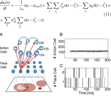
tc~0, tc~5ms and tc~?) are tested on a simulated Morris Watermaze task with variable start condition, a task known to involve hippocampus [51]. Hippocampus is represented as a population of place cells, with place cells centers organized on a rectangular grid. These model place cells project onto ‘action’ cells, putatively placed in the nucleus accumbens. The population of action cells represents the next action to be chosen by the model rat and is organized in a ring-like topology with lateral connectivity of the Mexican-hat type; see Figure 2.

Hippocampal place cells (HPC). Hippocampal place cells are modeled as Poisson neurons with a firing rate nf _{that is a} Gaussian function of the animal position in the environment:

nf_i(x,y)~n0exp {

(x{xi)2z(y{yi)2 2s2

!

ð10Þ

where (x,y) is the current position of the animal, (xi,yi) is the position at which thei-thplace cell gives the strongest response,

n0~110Hz is the maximum firing rate of the place cell. Unless marked otherwise, we consider in our simulations 100 such neurons placed on a grid of 10610 cells, with a distance of 10cm between two neighboring cells and withs~12cmbeing the width of each place field. The environment is a box of 1006100 cm. The ensemble activity of place cells encodes the position(x,y)of the animal.

Action cells (AC). Action cells are modeled as Leaky Integrate and Fire units [62], which are a special case of the Spike Response Model [20]. The change of the membrane potential of neuroniis given by

dui(t) dt ~{

1 tm

(ui{urest)z

X

j

X

tfj

jf_ija(t{tf_j){X tfi

g₀d(t{tf_i)z

zX

k wlc_ikX

tf k

a(t{tf_k{e)

ð11Þ

where tm~10ms the membrane time constant, urest~{70mV the resting potential,jf_ijis a stochastic variable that takes the value 1 with probabilityqijif the presynaptic place cellielicited a spike, and otherwise jij~0, wlcij the synaptic strength of the lateral

connections between neuronsiandj,tf_j andtf_k the spikes of the

presynaptic neuronj andk correspondingly,tf_i the postsynaptic spikes before time t andea small positive number. We note that the termtf_j in the second term on the right-hand side refers to

place cell firing whereastf_kin the fourth term refers to action cell firing. We assume that the postsynaptic current is a short pulse:

að Þt ~e0d(t{tf) ð12Þ

withe0~1mV andd(t) being the Dirac dfunction. If neuroni emits a spike, its membrane potential is reset by an amount

g₀~5mV. We note that with these definitions, our model is equivalent to a standard leaky integrate-and-fire model with pulse input and also a general case of the spike response model defined in Eq. (6).

In order to account for intrinsic noise or synaptic noise generated by additional presynaptic neurons that are not part of the model, we use a stochastic firing threshold [20,63], also known as escape noise. Action potentials of the postsynaptic neuroniare generated by a point process with stochastic intensity r_i~g(ui) where ui is an exponential function of the membrane potential [20,64]

r_i~g(ui)~r0exp ui{uh

Du

ð13Þ

where r₀~1/ms is the stochastic intensity at threshold, uh~{50mVthe formal firing threshold andDu~5mVthe width of the threshold region. We note that for the choice (13) the factor g’=g in the eligibility trace of Eq. (8) is a constant that can be absorbed in the learning rate. Unless stated otherwise, we use NAC_{~360action cells for our simulations.}

Lateral connections. The action neurons are connected in a ring with ‘‘Mexican hat’’-type lateral connections. A weakly localized feedforward input to action celliis sufficient, to cause within 25–200ms the formation of an activity blob. The location of the activity blob represents the next action of the rat. Because of the broad activity profile, not only the one neuron that is maximally active, but also neighboring active neurons can be reinforced during learning. For the sake of simplicity, we keep in our model the lateral connections fixed (i.e. they do not undergo synaptic plasticity) and use the equation:

wlc

ij~wEexp {

jhi{hjj2 2s2

!

{wI{w0 ð14Þ

withwlc

ij being the connection between neuronsiandj,hiandhj their corresponding preferred directions (the difference taken modulo 360o_{), s~17}o_{, w}

E~1:5 (weak connections) or wE§2 (strong connections) and wI~0:9. Local connections, i.e.

jhi{hjjvs

ffiffiffiffiffiffiffiffiffiffiffiffiffiffiffiffiffi

2ln wI wE

r

, are excitatory with w0~0while

connec-tions over a longer distance are inhibitory, Eq. (14) withw0~0:5. We have chosen parameters such that blob formation takes place already at the beginning of the learning procedure. The effect of the lateral connections is similar to a Winner-Take-All mechanism.

Figure 2. Hippocampal model.A: Schematic overview. Place cells

Decision making. At each location in the maze, the rat has to choose the direction of its next move. The decision is taken after a bump-like activity profile has been formed in the action layer. We suppose that the population of action cells is modulated by inhibitory background input in the theta-frequency range. If inhibition is strong, no activity profile is formed and neurons are inactive. While background inhibition drops to zero an activity profile develops, centered around the action neurons with strongest feedforward input - and these represent the action the rat is going to choose next.

In order to keep the model as simple as possible, we mimic the modulation of inhibition at theta-frequency algorithmically, by resetting every 200 milliseconds the activity of all action cells to zero. Otherwise, the dynamics is evolving freely according to the dynamical equations above. After 200 milliseconds, the rat takes its decision about the next action based on the population vector of the action cell firing rates. More specifically, the firing rate of action cells1ƒiƒNACis estimated from a low-pass of the spiking activity

_ ri~{

ri td

zYi(t) ð15Þ

wheretd is a time constant set at10ms(or200ms) andY(t)the entire postsynaptic train of the action cell defined as Y(t)~P

id(t{t f i), witht

f

i the fth firing time of thei-th action cell. The direction that the rat will follow is described by the angle

h in an allocentric coordinate system, i.e. relative to room coordinates and calculated from the population vector:

h~arctan

P

i

ricos (2pi=NAC)

P

i

risin (2pi=NAC)

0 @

1

A ð16Þ

whereNAC_{is the total number of action cells (typically 360 unless} otherwise stated), and2pi=NAC _{the direction of the i-th action} cell.his calculated after a decision timeTƒ200ms. In Figure 3 C–E, T is the moment when the total activity of all action cells

P

iriwH, withH~200Hz_{, which is achieved if, e.g. 10 cells fire} at more than 20Hz, a good indicator of when a decision (an activity bump) is formed. For all other simulations,T~200ms, but in general any of these conditions are possible for each case.

Watermaze performance

We perform simulations of a model rat navigating in a square maze of1m2_{, with a constant speed of 20cm/s. The rat performs a} number of trials, with each trial consisting of an attempt to find the goal within a time limit of 90 seconds. At the beginning of each trial, the rat is placed near one of the walls of the maze. Actions are chosen at theta frequency (every 200ms). Between two action choices, the simulated rat moves by about 4cm. The rewarded position (target) is at a random position near the central region of the maze and remains fixed at the same position within a set of trials whereas the initial position of the rat varies, as in the experimental paradigm [51,65,66]. Positive reward(R~1)is only given if the rat reaches its target and negative reward(R~{1)if it hits the wall. Thus, synaptic modifications take place either at the time the rat reaches the platform,tgoal, or at the time the rat hits a wall,twall. For an overview of the algorithm see Figure 4.

When a newset of trialsstarts, the positions of both the rat and the goal are reinitialized as well as the synaptic release of all plastic synapses in the model. Thus each newset of trialscorresponds to a different animal.

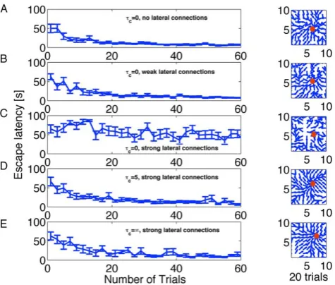
Speed of learning. The performance of the rat is measured by the time it takes to reach the target, corresponding to the escape latency in the experimental literature [51,65,66]. In the panels of Figure 3 A–E we plot the escape latency versus trials for three values of the parameter tc and three conditions of the mexican hat connections, zero (wE~0, wI~0 and w0~0), weak (wE~1:5, wI~0:5andw0~0) and strong (wE~2,wI~0:9andw0~0:5). For zero or weak lateral connections learning takes place within 20 trials with any value oftc(Figure 3 A,B). The performance is similar to that seen in experimental data [51] and previous models [52,55]. The standard deviation of the performance extracted from 10 repetitions of the learning experiment decreases while the task is learned.

Surprisingly, for lateral connections strong enough to form an an activity bump in the action cell layer, only the versions of the rule with a dominant Hebbian component (tcw0) are able to learn the task (Figure 3 D,E), but not the standard policy gradient rule for spiking neurons (tc~0, Figure 3 C). We believe that the critical parameter for a good performance of the policy gradient rule is neither the lateral connectivity nor the total input. Rather, it is a subtle interplay between the rule for the action choice (here: population vector based on firing rates) and the information encoded in the eligibility trace (see Discussion for more details).

In our model, actions depend on the population vector of the Action Cells calculated from the spike count about 200ms from each cell. Action cells, that have emitted most spikes, are most likely to dominate the action choice at a given place. Therefore, a standard Hebbian learning rule, that increases weights when pre- and postsynaptic neurons are jointly active, will set an eligibilty

Figure 3. Learning performance for different variants of the

learning rule.A. Left: Evolution of escape latency as a function of

trials, without lateral connections (wlc

ij~0) and Du~3mV. Right: Navigation map after 20 trials visualized in the water maze by a set of direction vectors. At each grid point (defined by the center of a place cell j) in the graph, we plot the normalized stochastic release probabilityqijfor fixedjin the form of a population vector denoting the direction the animal would most likely take at this location. The red circle marks the position of the hidden platform. The navigation map is less smooth than with the standard choice of parameters oftc~5ms or

tc~?, see D and E, Right. B. As in A with weak lateral connections,

tc~0andDu~5mV. C. As in A with strong lateral connections,tc~0 andDu~5mV. D. As in A with strong lateral connections,tc~5ms and

Du~5mV. E. As in A with strong lateral connections, tc~? and

Du~5mV. Initial release probabilities are set to 0.2; all other parameters as in Model architecture, Methods and Tables 1, 2.

trace that is strongest for the action neurons that have most likely determined the action at this location. If that action led to a reward, those weights would be strengthened. Thus, it is not surprising that the model withtc??does work. What would be the situation for the standard policy gradient rule with tc~0? As long as the expected number of spikes r_iT within the decision period of durationTis smaller than one, the termyi(t){ri(t)in the eligibility trace is positive for all neurons that have fired a spike – and these are exactly the neurons that determine the next action via the population vector. However, if the firing rates are higher, such a match between the memory kept in the eligibility trace and the chosen action is not guaranteed for insingletrials of the standard policy gradient rule (see Discussion for more details). We report that

the average instantaneous firing rate for the network without lateral connections, calculated as an average value among all action cells between the 20th and the 30th trial, isr~0:002Spikes/ms. For the same network but with weak lateral connections is r~0:006 Spikes/ms (three times more) and with strong lateral connections an order of magnitude higher, i.e. r~0:032 Spikes/ms. More importantly, the neurons inside the activity bump fire in Figure 3 C–D at a rate ofr~80 Hz yieldingrT&16 spikes,T~200ms. Thus, the eligibility trace of the most active synapses accumulates about 16 spikes of the postsynaptic neuron.

For the case of tc~5ms we compared the situation without baseline subtractionb~0and with a baseline subtractionb~R, and the results are similar (data not shown). However, if we follow

Figure 4. Learning algorithm.The decision timeTcan be either 200ms, as in most cases, or can be based on a flexible criterion (Figure 3 C–E), see

Results.

learning for more than 100 trials, the factor R{R increases long-term stability, as expected.

Navigation map. Given the rat’s location, the direction of the next move is decided by the population vector of the action cells. Suppose that the rat is in the center of the place field of cellj. Then the population activity of the action cells is, to a large degree, controlled by the strength of the synapses connecting place celljto the different action cells: the stronger the synaptic weightwijto an action celli, the more likely that the action represented byiwould be chosen. We therefore use the population vector of the synaptic strength of the feedforward connections from a given place cell to visualize the direction of motion starting at that location. The combination of vectors gives a flow map, corresponding to the navigation map of the rat. In Figure 3 A–E right hand side we show the navigation map after the 20th trial for differenttcvalues and lateral connections. It is noteworthy that the quality of the navigation map is increased under the presence of strong connections (and tcw0). Figure 5 shows the evolution of the navigation map of the rat fortc~5msafter 1, 10 and 50 and 100, with A–C depicting preferred directions as normalized vectors and D–F as non-normalized vectors. A–C show that already within 10 trials the simulated animal has developed a strategy for reaching the goal, and D–F show the relative strength of the population activity, which increases as the animal moves closer to the target. Adequate learning has been achieved, if for any starting condition the flow is towards the target zone. We find that already after 10 trials, a rough strategy for the Morris watermaze task has been developed, which is refined during subsequent trials. Figure 6 confirms that trajectories become smoother during learning. A sequence of 3 action choices has a strong random component at the beginning but is nearly continuous after 100 trials.

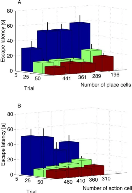
Performance vs number of place and action cells. How does the performance depend on the number of place and action

cells? For place cells, we require that the surface of the water maze will be sufficiently covered by neurons with overlapping receptive fields. This continuous space representation (due to overlapping receptive fields) leads to simultaneous learning of nearby neurons, resulting in no significant change in performance even when doubling the number of neurons in each dimension, see Figure 7 left. Similarly, a minimum number of action cells is required such that the activity profile will be created, but increasing the number of cells beyond 300 cells or so does not change the performance. The reason is that the activity profile has always roughly the same width (about 30 degrees) in action space. Adding more cells just increases the number of cells in the activity bump. In Figure 7 right we plot the average time it takes the rat to reach the hidden platform at the 5th, 25th and 50th trial versus number of action cells. We note that the performance does not significantly change. This is in contrast to standard reinforcement learning in discrete state and action spaces where increasing the number of states or actions increases the number of free parameters, so that learning becomes slower [1].

Discussion

We presented a spike-based reinforcement rule which combines a global reward signal with two local factors available at the site of the synapse. The first local component is a contribution generated by presynaptic spike arrival and enters the update rule in the form of the EPSP. The second local component depends positively on postsynaptic spike firing and negatively on the postsynaptic membrane potential. The relevance of the membrane potential decreases withtc and vanishes fortc??. The third factor of the learning rule is the global reward signal that can be associated with neuromodulators such as dopamine [22]. Thus the eligibility trace which combines the two local factors marks the synapse that can undergo LTP or LTD. The actual weight change is implemented only after confirmation by a global reward signal that may arise with a significant delay. Such a picture has interesting relations to the model of synaptic tagging and capture [27] where synaptic connections undergo preliminary changes into early LTP or LTD that decay unless they are stabilized if plasticity related protein is available. Synthesis of these plasticity related protein can occur with a delay and requires neuromodulators such as dopamine [28,61].

Global factors, neuromodulators, and TD-learning In the introduction we mentioned two classes of theoretical reinforcement learning algorithms, that is, temporal difference

Figure 5. Navigation map of the rat visualized in the water maze by a set of direction vectors, fortc~~~~~~~~~~~~~~~~~5ms.Panel A depicts the map formation after 1 trial, B after 10 trials and C after 50 trials. The simulated animal has developed a rough strategy to reach its goal already within 10 trials. For details on how the navigation map is calculated, see Figure 3. Learning rate decays as a function of mean reward. Preferred directions are plotted as normalized vectors. In D–F we plot the same navigation maps with non normalized vectors. While F seems to contain no information about preferred directions near the wall (due to scaling of arrows), the normalized version C confirms that the simulated animal has developed a strategy for all positions in the maze.

doi:10.1371/journal.pcbi.1000586.g005

Figure 6. Sequential formation of actions.Spiking activity (dots) of

(TD) learning methods on one side [1,43] and policy gradient methods on the other side [39,40]. Our model task and model architecture would allow to test both types of algorithm in the form of a three-factor rule (see [45,52–54] for examples of a TD algorithm for this task). One major difference between the TD algorithms and the algorithm in this paper lies in how the global factor encodes neuromodulatory feedback about the reward. In the case of TD-learning, the global factor expresses the difference between the reward received and the expected reward (where the expected reward is calculated from the temporal difference between reward expectations of subsequent states [1]), whereas in the case of the gradient learning algorithm of this paper the global factor correspond to reward itself, possibly after subtraction of a baseline. Here we used a variant of the idea of a baseline, since we subtracted the mean reward averaged over ordermprevious trials, see also [41]. Subtracting the expected reward should help rapid re-learning in case of the change of the learning task (e.g., by

moving the escape platform to a different location) [67]. Similar to TD learning the global factor can be interpreted in this case as reward minus expected reward. In contrast to TD learning, the expected reward arises from a running average, rather than a difference in reward expectation across different states as in spike-based TD algorithms [37,45]. Experiments on dopaminergic neurons suggest that the phasic dopamine signal indeed encodes a TD-like error signal [22] although other interpretations of the dopamine signal [68] and the involvement of other neuromodu-lators is also possible [69].

Our spike-based navigation model features a continuous description of state and action. Unlike traditional TD models with discrete state and action space, increasing the number of neurons while keeping the width of place fields and the width of lateral interactions between action cells constant) does not change the performance of our model. In addition, the model provides insight in studying decision making in the context of navigation. We hypothesized that activity is modulated at theta frequency. Note that we implemented an extreme situation where the action choice is taken at the end of each theta cycle. However, it is easily possible to have the rat take an action as soon as the activity profile is formed. The time necessary to create an activity profile determines then a minimal time for deciding a new action. If this is so, then our model predicts that the time it takes to choose the next action is much faster after learning than before learning, because activity profiles are more rapidly formed with strong feedforward input - as it would occur after learning.

Morris water maze task

To test the potential of our spike-based reinforcement rule, we have applied it to a biologically relevant navigation problem, i.e., the Morris water maze task with variable start condition [51]. Our model which is based on a simplified model of place cells and action cells reproduces behavioral data of real rats in terms of escape latency versus learning time. The model consists of about 700 spiking neurons, in two layers and includes both feedforward and lateral connections. In the first trial, the model rat moves in a random trajectory and finds the hidden platform by exploration. Across several trials, approach paths towards the platform are reinforced, so that the escape latency is reduced.

A positive reward is delivered when the model rat reaches the target location. In the model, we also use negative reward at the boundaries of the maze so that the simulated rat will learn to avoid the walls. This aspect does not reflect the fact that, normally, during development (or even because of reflexes present at birth) we could assume that the rat already knows how to avoid obstacles prior to the start of the watermaze task. However, since we did not want to include into the model prior knowledge about obstacle avoidance, we let the simulated rat ‘discover’ the effect of the walls. Since our model assumes the existence of place cells, we must assume, however, that the rat has had some pre-exposure to the environment long enough to establish place fields. Experiments have shown that place fields are established during a first exploration of the environment, so that during the learning task, they can be considered as given. Moreover, typical experiments require prior habituation of the animal to the environment, so that place cells may be formed. A model where place cells are learned from visual input and path integration is also possible [53].

While in our model place cells can be easily linked to cells in hippocampus, a direct identification of the action cells with the biological substrate is more problematic. In rodents, navigation in water maze task involves two competing pathways [70–72]. The first one is involved in taxon navigation (e.g., approaching a visible target, which could be achieved with stimulus-response habits [73]

Figure 7. Scaling properties of the network.A: Average time it

takes the rat to reach the hidden platform at the 5th, 25th and 50th trial versus number of place cells. B: Average time it takes the rat to reach the hidden platform at the 5th, 25th and 50th trial versus number of action cells. Error bars show standard error for the mean. Note the improvement as the number of place cells is increased. This is due to the systematic formation of an activity bump in the presence of stronger input. The same parameters were used in producing all sets of these simulations: l~0:0008, tc~5ms, mr~20, te~60s, td~10ms,

also called response learning [71]) and associates visual input directly with motor actions. It is independent of hippocampus and the action choice for this navigation strategy can presumably be linked to the the dorsal striatum of the basal ganglia (caudate-putamen in the rat). The second one is concerned with locale navigation (also called place learning [71] or cognitive map [74]) and this is the relevant pathway in the context of the present model. It relies on hippocampus [51,70,71] where the activity of place cells presumably encodes the location of simulated animal. The choice of motor actions is presumably encoded in the nucleus accumbens (NA) of the ventral striatum where our hypothetical action cells could be located. The Mexican hat connectivity between action cells is a simplification of a more complex wiring scheme, where excitatory neurons project to inhibitory neurons, which in turn inhibit other action cells that encode for ‘‘different’’ directions, see for example a biologically plausible winner-take-all [75]. However, to reduce the connectivity in our network, we chose to simulate the equivalent but simpler Mexican hat scheme. One limitation of the model is that learning only takes place in the presence of a reward signal with the consequence that learning can only occur in a limited radius around a reward. The radius is related to the time scale of the eligibility trace, governed by the time scalete. In a large environment where at a fixed speedv0it takes much longer than te to traverse the environment, information about the target falls off exponentially with a spatial scaler~tev0. In our case we would encounter this limit only if the environment were scaled by a factor significantly larger than two. In a TD framework, the situation would be different: even without an eligibility trace, information about the presence of the reward can slowly diffuse across the landscape of estimated reward expectation valuesV(x)wherexis the position, even beyond the radiusrdiscussed above. This slow diffusion of reward information is possible because the update is not proportional to the reward itself, but to a factor d~RzcV(x’){V(x) where V(x’){V(x) gives the difference between the reward estimation at locationx’ and that of the previous locationxand 0vcv1is the discount factor. An implementation of a TD learning structure in spiking neurons is possible using the actor-critic scheme [37,45]. If a TD algorithm is implemented in discrete time with time stepsD, and if the rat runs as before at a constant speedv0, the distance travelled between two time steps isDx~v0D. After convergence, the value function decreases exponentially with the distance from the target on a lenght scale r’~{v0D=lnc&v0D=(1{c). (In other words, once the exponentially decayingVdependence is reached, thedin the update rule vanishes). A comparison with the result in the previous paragraph shows that the time scale te of the eligibility trace in our model plays a role similar toD=(1{c) in the TD model. The role of the eligibility trace has been extensively discussed in [35]; in our interpretation the eligibility trace is implemented in the synapse and its time constantte corresponds to the decay time of some biochemical substance.

The parametertcis an ad-hoc parameter that allows us to vary the behavior of the learning rule from pure Hebbian to optimal in the sense of policy gradient theory. We do not wish to explicitly associate it with a biological substrate, but in our model it would be closely related to the voltage dependence of LTD.

Recently, the influence of neuromodulators on spike-timing dependent synaptic plasticity has been investigated in a small number of studies [31,76]. These studies show that dopamine acts on the temporal profile of STDP, rather than a simple scaling of STDP. This result is in contrast to some of the assumptions of standard reward-modulated STDP [35,36], but also in disagree-ment with policy gradient rules [33,34,38] and the learning rule discussed in this paper. For plasticity in the cortico-striatal synapse

[31], but not for glutamatergic synapses in hippocampal neurons [76], dopamine is necessary for synaptic plasticity. In other words, learning is gated by the presence of dopamine. The plasticity rule in the cortico-striatal synapse is in that respect similar to the reward-gated plasticity rules in the present paper. Interestingly, the striatum is potentially involved in action selection.

It should be noted that in standard cortical STDP experiments [77,78] the level of dopamine and other neuromodulators is not explicitly controlled and a background level of dopamine cannot be excluded. Therefore, it is unclear whether cortical STDP is unsupervised or shows a, possibly weak, dependence upon neuromodulators.

Limitations of policy gradient methods

An important parameter in our family of learning rules is the parametertc, that tunes the learning rate such that for neurons that fire at high learning rates LTD is reduced. To see this, consider an instantaneous firing rater_i(t)&1=tc. Then the term r_i(t)=½1ztcri(t)converges to1=tcvr_i. Hence, the decrease of the eligibility trace in the absence of spikes is limited. Note that because ofr~g(u)high rates correspond to large depolarizations of the membrane potential. Fortc??, the termri(t)=½1ztcri(t) vanishes, and the membrane potential u no longer enters the update of the eligibility trace. In this case the eligibility trace pick up Hebbian correlationsY(t)e(t{tf_j) between EPSPs caused by presynaptic spike arrival and postsynpatic firing.

The casetc~0corresponds to the learning rule derived from the reward maximization as shown in the methods section, i.e.,

r_i(t)=½1ztcri(t)~ri(t). For tc~0 the two postsynaptic terms, i.e., spike firing and voltage dependence cancel each other on average, because spikes are generated with the stochastic intensity

r_i~g(ui), hence SYi(t){ri(t)T~0 where angular brackets denote expectation values. However, a specific realisation of a spike train (e.g., one with more spikes than expected) may lead to a reward whereas another one (with less spikes than expected) does not. In this case only the rewarded one is learned, making it more likely that the same spike train is reproduced again for the same input [34]. In fact, a large class of learning rules for conditioning can be explained as a reinforcement of the covariance between reward and a noise-induced variation of the output [79].

There are three reasons why the standard policy gradient rule withtc~0derived from reward maximization is not applicable in our scenario.

(i) Large learning rate. The learning rule derived from reward optimization is a batch rule, i.e., it assumes averaging across several realisations and many inputs. For the transition to the online rule we had to assume a very small learning rate so as to make the learning self-averaging. If learning is slow, then thousands of trials are needed before the weights change significantly, so that online and batch have nearly the same effect. In order to explain biological learning paradigms, we need, however, to achieve learning after as few as ten trials. If we work with a large learning ratel, then terms of the formYi(t){ri(t) that average away in the batch rule, can make a big contribution in the eligibility trace of each single trial and can cause weight changes that are not causally linked to the reward. Thus the eligibility trace encodes noise, rather than relevant correlations. With small learning rate, these correlations would average away (and only those systematically linked to the reward would survive), but with a big learning rate these changes act like a diffusion process. Moreover, the effect of the diffusion increases with the number of spikes in the decision window and therefore is highest for neurons having a large firing rate r_i. Large firing rates r_i

bump, because strong lateral input is added to strong feedforward input. Hence the eligibility trace is most noisy in the center of the bump, as shown in Figure 8 B.

(ii) Decision by firing rates, not by spikes. The close relation between reward-maximisation by policy gradient rules and supervised learning shows that the spike-based rule withtc~0is optimal to learn a specific spatio-temporal spike pattern [34]. However, what counts for the action choice in our simulations is the firing rate accumulated over 200ms. To understand the importance of this distinction let us consider two Poisson neurons coding for actions ‘left’ and ‘right’, respectively. The action ‘right’ is the rewarded one. Suppose the neurons receive inputs that drives the neurons coding for ‘left’ at an intensityr_left~5Hzand the other atr_right~50Hz. Suppose, because of intrinsic noise, the neuron coding for ‘left’ fires 2 spikes in a decision interval of T~200ms, while the neuron coding for ‘right’ fires 9 spikes in the same time interval. If actions are chosen according to maximal firing rates, the neuron coding for right wins, the system performs the ‘right’ action and receives reward. However, the term

ÐT

0½Y(t){r(t)dt is negative for the neuron coding for ‘right’ and ‘positive’ for the neuron coding for ‘left’. Hence, after reward is received action ‘right’ is weakened, while action ‘left’ is reinforced, in contradiction to the fact that action ‘right’ is the correct one that should be reinforced. To put it differently, action neurons have to learn that (a) precise spike timing is irrelevant and that (b) even the absolute rates are irrelevant because all that matters is the firing rate relative to those of the other neurons. Since the policy gradient rule is desigend to learn precise spatio-temporal spike patterns, it is not ideally suited for our paradigm. In contrast, reward-modulated Hebbian learning just make the neurons that fired at high rate (and influenced the action) fire at

even higher rates. In the specific task we are considering this happens to be a viable strategy.

(iii) Populations of neurons, not single neurons. Furthermore, because of the formation of an activity bump and the readout by a population vector the decision about actions is taken by apopulation of neurons rather than individual neurons. Learning in popula-tions suffers from the problem that firing of individual neurons may differ from the majority vote that led to the actions, so that giving appropriate feedback is nontrivial [80].

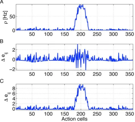
Figure 8 illustrates the detrimental interaction of points (i)–(iii) for the standard policy gradient rule. We focus on a presynaptic neuronjwhich codes for the current location of the rat so that synapses from j to all action neurons i are active. The instantaneous firing rater_irepresents the activity bump (Figure 8 A). Despite the fact that the termYi(t){ri(t)has an expectation value of zero, the term Yi(t){ri(t) gives a non-neglibible contribution in each trial, see also Figure 1 C – as it should be since policy gradient rules need to exploit fluctuations. However, we would like to emphasize two aspects. First, the standard deviation ofjYi(t){ri(t)jgrows with time, similar to a diffusion process. Second the diffusion constant increases with the instantaneous rater. Therefore the deviation from the expected valueSYi(t){r_i(t)T~0increases with the expected number of spikesr_iTthe neuron emits during the decision interval of length T. The eligibility trace is sensitive to this deviation. In the case of our action learning model, the consequence of the above argument is that the set of significantly positive eligibility traceseijfor fixed presynaptic neuronjincludes not just action neurons within the activity bump, but also those representing other directions; see Figure 8 B. Moreover, the variation of eligibility traces between neighboring neurons inside the activity bump is big, because the expected number of spikes is higher for neurons inside the activity bump. In particular, several synapses from a fixed presynaptic neuron onto neurons in the bump have eligibility traces that are significantly negative (corresponding to the fact that some neurons in the bump fire less spikes than expected from the firing rater_i, see point (ii) above). This leads to the problem that eligibility traces of individual neurons do not reflect the action choice represented by the population of active neurons [80]. Simply speaking, neurons inside the bump are those that determine the action even though their eligibity trace can be negative.

The parametertcin our learning rule gives a systematic positive bias of the postsynaptic term for those postsynaptic neurons that have a large firing rate. Thus the eligibity trace is maximal for neurons within the bump of activity, i.e. for those representing the action that is actually chosen; see Figure 8C. Hence, if the sequence of actions leads to a reward later on, the synpatic weights between those presynaptic place cells and postsynaptic action cells that actually led to the sequence of actions are maximally strengthened. Because of the bounds on the weight dynamics, these weights will eventually converge towards a release probability ofqij~1. We note that all neurons outside that activity bump have very low activity, so thatYi(t){½ri(t)=(1ztcri(t))&Yi(t){ri(t) has a zero average and only small fluctuations. Hence, a learning rule withtcw0_is expected to work better in the case of large learning ratesl, and high firing ratesr, and a decision criterion based on a population vector calculated over a long time period.

In a general spike-based learning problem where the aim is to learn a spatio-temporal spike pattern, the high variability of eligibility traces would allow to explore a large space of firing patterns. However, in our case with lateral interactions and decisions based not on detailed firing patterns, but only on population vector data integated over 200ms, the bias towards high activities identifies neurons in the bump that participate in the action choice.

Figure 8. Action cell activity and eligibility trace.A: Snapshot of

mean firing rate of action cells during one of the trials while the simulated rat is in the center of the place field of cellj. The chosen action is a movement in direction200o_{. B and C. At this instance, the} momentary value of the eligibilityeijis plotted as a function ofifor fixedj(fixed presynaptic location). B: For the rule withtc~0the profile of eligibility traces is stochastic with zero mean and maximum variance inside the activity bump. C: Fortc~5msthe profile of eligibility traces reflects the activity profile shown in A.

Indeed, a learning rule withtc~0does work in the situation where (a) there are no lateral interactions between the action cells or (b) decisions are based on less than one spike per neuron on average. In the latter case, every spike is unexpected, and basing a decision on the population vector chooses an action that is indeed caused by a fluctuation.

In principle four action neurons would be sufficient to encode the direction of the next action (e.g., [45,53]). In this case, learning rules based on either policy gradient [45] or naive Hebb [53] work. However, it is likely that in biological brains actions are encoded by large populations of neurons. In order to achieve fast learning despite a large population of action neurons, action neurons must share information during learning – and this can be achieved by the formation of activity bumps. The results of this paper show that in the presence of activity bumps and population vector read-out based on spike counts, the spike based policy gradient rule no longer works, whereas a rule with a bias towards Hebbian correlation does.

From a technical point of view, neither stochastic synapses nor voltage dependent plasticity is critical for the function of the model, however they are both desirable properties for the biophysical plausibility of the rule. In our model, the stochastic release probability of the synapses is hard-bounded in order to maintain reasonable values, for a biophysical implementation of such bounds see [46].

Also a reset it is not necessary to take place exactly every 200msec; in principle may occur at any point that the activity bump is formed. We require to reset the activity in the action neurons layer only (or equivalently we could clamp the AC activity for say 10ms) so that the activity profile will not become ‘‘sticky’’, but in no other way the learning would be affected. Without reset, the rat will end up again learning the position of the platform, but its movements will become more curved. A negative input would be desirable after a decision is formed so that at the beginning of the learning the next action will not depend on the previous one. This negative input may arrive at any point after a decision (activity bump) has been formed. We chose 200ms so that this could coincide with the theta rhythms, but it could have been 150ms or 300ms, or a random interval (as we demonstrate in simulations).

Methods

Policy gradient methods [39,40] have been applied to spiking neurons several times and result in spike-based formulations of reward-based learning [32–34,38]. In the following subsection we derive again the same rule, but with the aim to show that the derivation holds even in a network of spiking neurons with strong lateral connectivity (see also a comment in [40]). In the following two subsection we make the transition to an online formulation with eligibility traces and stochastic synaptic transmission. In subsection we leave the policy gradient framework by introducing the parametertc in order to enable a smooth transition between the standard policy gradient rule and a naive Hebbian rule that measures directly correlations between presynaptic spike arrival and postsynaptic firing on the time scale of the EPSP. The rule used in the main body of the paper is a mixture between policy gradient and naive Hebbian rules.

Derivation of the learning rule

To derive a learning rule for a highly connected network with action cellsiwith lateral connections receiving from input from place cellsj, we shall first consider a restricted scenario where the rat always starts a trial in the same initial location and is left to move around for a fixed durationT. We shall denote byxT (yT) the spatio-temporal spike pattern generated during this time by all place (action) cells. The reward, administered at the end of each trial, depends on the trajectory of the rat in the water maze. Given the fixed initial location, this

trajectory is determined by the firings of the action cells. So we write reward as a functionR(y_T){b, where b is the reinforcement baseline [39], without explictly noting the dependence on the initial position of the rat. Expected reward then is [32,34]

SRT~

ð

dxTdyTðR(yT){bÞPw(xT,yT) , ð17Þ

herewdenote the strengths of the synapses connecting the action to the place cells, and Pw(xT,yT) is the probability that the network generates the total spike pattern(xT,yT).

In our model Pw(xT,yT) can be decomposed as (see also Decomposition of probability):

Pw(xT,yT)~ P

j gj(xT,yT)

P

i hi,wi(xT,yT)

: ð18Þ

Here hi,wi(xT,yT) is the function giving for the action cell ithe single neuron probability that it generates its spike train yi,T~ft1i,t2i,. . .gwith an input consisting of all the other spikes produced by the network. Similarly,gj(xT,yT)is the single neuron probability function for the spike train produced by thej-thplace cell given its input (determined by the other spikes in the network). Note that the above product form does not imply that the spike trains are statistically independent. This is obviously not the case: First, due to the lateral connections between the action cells, and, more importantly, due to the simple fact that the action cells decide on the rats trajectory and thus influence the firing of the place cells. The product form simply represents the fact that the internal stochastic processes which modulate the translation of presynaptic input to postsynaptic output are assumed to be independent between different cells. In other words,giventhe input spikes from all other neurons and its own previous spikes up to timet, the neuronidecides locally whether it fires betweent andtzDt or not (i.e., we activate an independent random process for each neuron in each time step of the simulation), see section Decomposition of probability.

An explicit form forgj(xT,yT)would be rather complicated, due to the involved calculations mapping the action cell firings to the trajectory of the rat. Luckily, we just explicitly needhi,wi(xT,yT). Note, and this is in fact the crucial feature of the decomposition, thathi,wi does not depend on all feed-forward weights, but only on the weight vectorwiof the synapses actually projecting onto neuroni.

To calculate the gradient of the expected reward (17), we first rewrite the probabilityPw(xT,yT)as

Pw(xT,yT)~

Pw(xT,yT) hi,wi(xT,yT)

hi,wi(xT,yT) ð19Þ

and note that in view of (18) the term in square brackets in fact does not depend on wi (even if this is not apparent from the notation). Now, for the synapse connecting place celljto action cellithe gradient calculation is

L LwijSRT~

ð

dxTdyTðR(yT){bÞ L Lwij

Pw(xT,yT) hi,wi(xT,yT)

hi,wi(xT,yT)

~

ð

dxTdyTðR(yT){bÞ

Pw(xT,yT) hi,wi(xT,yT)

_L

Lwijhi,wi(xT,yT)

~

ð

dxTdyTPw(xT,yT)ðR(yT){bÞ L Lwij

loghi,wi(xT,yT)

ð20Þ