Modelling the influence of non-minimum phase zeros on gradient based linear iterative learning control

This is a repository copy of Modelling the influence of non-minimum phase zeros on gradient based linear iterative learning control.

White Rose Research Online URL for this paper: http://eprints.whiterose.ac.uk/74693/

Monograph:

Owens, D.H. and Chu, B. (2009) Modelling the influence of non-minimum phase zeros on gradient based linear iterative learning control. Research Report. ACSE Research Report no. 991 . Automatic Control and Systems Engineering, University of Sheffield

Reuse

Unless indicated otherwise, fulltext items are protected by copyright with all rights reserved. The copyright exception in section 29 of the Copyright, Designs and Patents Act 1988 allows the making of a single copy solely for the purpose of non-commercial research or private study within the limits of fair dealing. The publisher or other rights-holder may allow further reproduction and re-use of this version - refer to the White Rose Research Online record for this item. Where records identify the publisher as the copyright holder, users can verify any specific terms of use on the publisher’s website.

Takedown

If you consider content in White Rose Research Online to be in breach of UK law, please notify us by

Modelling the Influence of Non-minimum Phase Zeros on

Gradient based Linear Iterative Learning Control

David H Owens, Bing Chu

Department of Automatic Control and Systems Engineering,

University of Sheffield,

Mappin Street, Sheffield, S1 3JD, UK

Eric Rogers, Chris T Freeman, Paul L Lewin

School of Electronics and Computer Science,

University of Southampton,

Southampton SO17 1BJ, UK

Research Report No. 991

Department of Automatic Control and Systems Engineering The University of Sheffield

Mappin Street, Sheffield, S1 3JD, UK

Modeling the Influence of Non-minimum

Phase Zeros on Gradient based Linear

Iterative Learning Control

David H Owens, Bing Chu

Department of Automatic Control and Systems Engineering, University of Sheffield, Mappin Street, Sheffield S1 3JD, UK

Eric Rogers, Chris T Freeman, Paul L Lewin

School of Electronics and Computer Science, University of Southampton, Southampton SO17 1BJ, UK

Abstract

The subject of this paper is modeling of the influence of non-minimum phase plant dynamics on the performance possible from gradient based norm optimal iterative learning control algorithms. It is established that performance in the presence of right-half plane plant zeros typically has two phases. These consist of an initial fast monotonic reduction of theL2 error norm followed by a very slow asymptotic

convergence. Although the norm of the tracking error does eventually converge to zero, the practical implications over finite trials is apparent convergence to a non-zero error. The source of this slow convergence is identified and a model of this behavior as a (set of) linear constraint(s) is developed. This is shown to provide a good prediction of the magnitude of error norm where slow convergence begins. Formulae for this norm are obtained for single-input single-output systems with several right half plane zeroes using Lagrangian techniques and experimental results are given that confirm the practical validity of the analysis.

Key words: non-minimum phase plants, iterative learning control, optimization.

1 Introduction

Iterative learning control (ILC) is a technique for controlling systems operat-ing in a repetitive (termed trial-to-trial, iteration-to-iteration or pass-to-pass) mode with the requirement that a reference trajectory r(t) defined over a fi-nite interval (trial or pass length) 0 ≤ t ≤ α is followed to a high precision. Examples of such systems include robotic manipulators that are required to repeat a given task to high levels of accuracy, chemical batch processes or, more generally, the class of tracking systems.

Since the original work [1] in the mid 1980s, the general area of ILC has been the subject of intense research effort. An initial source for the literature here are the survey papers [2], [3] and [7]. A key point here is that many linear model based algorithms have also seen experimental benchmarking.

One class of widely considered algorithms (e.g. [5] and [6]) are “gradient based” i.e. iterate to produce the desirable property of reducing error norm magnitudes from trial-to-trial. One wide class of such algorithms using both function and parameter optimization methods is reviewed in [7]. As in all control algorithms, including the familiar feedback control paradigm, there are limitations as to what ILC can achieve depending on the characteristics of the plant. In particular, the structural properties of the plant are critical to what can be achieved. This paper, motivated by results first given in [4], uses standard tools from functional analysis in a Hilbert space to investigate the effects of non-minimum phase zeros on the convergence behavior of gradient based algorithms using the so-called norm optimal ILC (NOILC) approach [5]. This algorithm has the property of guaranteeing, for a wide class of linear systems, convergence of tracking errors to zero (in norm) but has been observed to exhibit a slow convergence behaviors for non-minimum-phase systems. The aim of the analysis in this paper is to provide a model of this observed behavior with a view to predicting its main parameters. The validity of the theoretical results in predicting observed phenomena is verified by experimental results obtained from an electro-mechanical testbed.

2 Background

Definition 1 Consider a dynamic system with input u and output y. Let Y and U be the output and input function spaces respectively and let r ∈ Y be a desired reference trajectory for the system. An ILC algorithm is successful if, and only if, it constructs a sequence of control inputs {uk}k≥0 which, when

output sequence {yk}k≥0 with the following properties of convergent learning

lim

k→∞yk=r, klim→∞uk=u∞ ∈ U

Here convergence is interpreted in terms of the topologies assumed in Y and U respectively.

Note that this general description of the problem allows a simultaneous de-scription of linear and nonlinear dynamics, continuous or discrete plant with either time-invariant or time varying dynamics.

Let the space of output signals Y be a real Hilbert space andU also be a real (and possibly distinct) Hilbert space of input signals. The respective inner products (denoted byh·,·i) and normsk · k2 _{=h·,·i are indexed in a way that}

reflects the space if it is appropriate to the discussion e.g. kxkY denotes the norm of x∈ Y.

The dynamics of the systems considered here are assumed to be linear and represented in operator form as

y=Gu+d

where G : U → Y is the system input/output operator (assumed to be bounded and typically a convolution operator) and d is a term describing initial condition or other trial independent effects such as disturbances. If r ∈ Y is the reference trajectory or desired output then the tracking error is defined as

e=r−y=r−Gu−d

This paper considers the NOILC algorithm of [5] which, on completion of trial k, calculates the control input signal on trial k+ 1 as the solution of the minimum norm optimization problem

uk+1 = arg min_u

k+1{Jk+1(

uk+1) : ek+1 =r−yk+1, yk+1 =Guk+1+d}

where the performance index, or optimality criterion, is

Jk+1(uk+1) =kek+1k2Y +kuk+1−ukk2U (1)

The initial control u0 ∈ U can be arbitrary in theory but, in practice, will be

This problem can be interpreted as the determination of a sequence of control inputs with the properties that, on trialk+ 1, (i) the tracking error is reduced in an optimal way; and (ii) this new control input does not deviate too much from the control input used on trial k. The relative weighting/importance of these two objectives can be absorbed into the definitions of the norms inY and U.The control input on trialk+ 1 is obtained from the stationarity condition, necessary for a minimum, by Fr´echet differentiation of (1) with respect touk+1

as

uk+1 =uk+G∗ek+1, ∀k ≥0 (2)

whereG∗ _{is the adjoint operator forG. This leads easily, usingy=Gu+dand} e=r−y, to the following formulae for the change in error from trial-to-trial

ek+1−ek =−GG∗ek+1, ∀k ≥0 (3)

and hence

ek+1 = (I +GG∗)−1ek, uk+1 =uk+G∗(I+GG∗)−1ek, ∀k≥0 (4)

Now consider the special case of a differential linear time-invariant plant mod-eled by the state-space triple {A, B, C} operating over a time interval [0, α] (with state, input and output y(t), x(t), and u(t) respectively). In this case, with input and output spaces being L2[0, α] spaces with appropriate norms,

G is defined by the equation

(Gu)(t) =C

t Z

0

eA(t−τ)Bu(τ)dτ, d(t) =CeAtx(0) (5)

and the cost function takes the form

Jk+1= α Z

0

{eT

k+1(t)Qek+1(t) + (uk+1(t)−uk(t))TR(uk+1(t)−uk(t))}dt (6)

where the weighting matrices Q and R are symmetric positive definite.

as a known disturbance on trial k+ 1). If we assume full knowledge of the state vector, the optimal input on trialk+ 1 is then

uk+1(t) = uk(t)−R−1BT[K(t)xk+1(t)−ξk+1(t)] (7)

where the feedback gain matrixK(t) satisfies the Riccati differential equation

˙

K(t) =−AT_{K(t)−K(t)A+K(t)BR}−1_BT_K(t)−CT_QC

K(α) = 0 (8)

and the predictive or feedforward term ξk+1(t) is generated by

˙

ξk+1(t) =−

A−BR−1BTK(t)T ξk+1(t)−ζ CTQ ek(t)

with terminal coniditon

ξk+1(α) = 0

The predictive term in this algorithm driven by a combination of the tracking error and the input on the previous trialkand also the reference signal. This is therefore a causal ILC algorithm consisting of current trial full state feedback combined with feedforward from the previous trial output tracking error data. This representation of the solution is causal in the ILC sense because the costate system can be solved off-line, between trials, by reverse time simulation using available previous trial data. The differential matrix Riccati equation for the feedback matrixK(t) needs to be solved only once before the sequence of trials begin. Also by reducingRto infinitesimally small values, high gain state feedback can be achieved which generates, intuitively, maximum convergence rates whilst satisfying the stability constraint. This is in contrast to high gain output feedback which cannot be used in practice due to instabilities arising from right-half plane zeros.

Norm optimal ILC has been shown ([5]) to have the following convergence properties for the error sequence {ek} and input sequence {uk}:

(1) The change in inputuk+1−uk converges in norm to zero.

(2) If the input {uk} converges, the limit is the input that minimizes the

error norm ||r−Gu−d||2 _{(where for ease of notation we have omitted}

explicit mention of the underlying function space(s)).

(3) The error sequence generated by (1) is monotonically decreasing in norm. (4) The error norm converges monotonically to zero if the reference signal is

The algorithm [5] is hence universally convergent and universally applicable in theory and is known to be capable of excellent convergence properties. This has been seen in extensive simulation work and, most importantly, in experimental benchmarking on a gantry robot [11] and experimental applications including an accelerator based free electron laser [12]. Both applications are minimum-phase. Non-minimum phase properties are the subject of this paper which also provides experimental verification of these results using a non-minimum-phase electro-mechanical system.

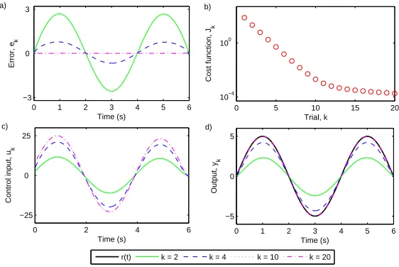
For a simple simulation example, Figure 1 shows the results of applying this ILC algorithm to the minimum-phase plant

G(s) = s+ 1 (s+ 2)(s+ 3)

with r(t) = 5 sin (π

2t) and in the cost function Q = 20, and R = 1. The

good convergence behavior is clearly visible with several orders of magnitude reductions inJ (and hence error norm) in the first 10 trials before convergence rates reduce.

0 1 2 3 4 5 6 −3

0 3

Time (s)

Error, e

k

0 5 10 15 20

10−4 100

Trial, k

Cost function, J

k

0 2 4 6

−25 0 25

Time (s)

Control input, u

k

0 1 2 3 4 5 6 −5

0 5

Time (s)

Output, y

k

r(t) k = 2 k = 4 k = 10 k = 20

a) b)

c) d)

Fig. 1. NOILC performance from a typical minimum phase system: a) error,ek, b)

cost function,Jk, c) control input,uk and d) output,yk.

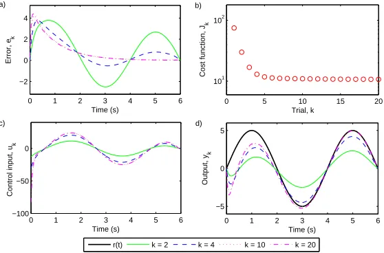
with only very small changes from trial-to-trial. For all practical purposes, (i) the input after the 6th trial barely changes and hence (ii) the error appears to be converging to a non-zero value. The problem is that the non-zero error “achieved” is, in this case, only an improvement of a factor of approximately 10 in norm over the initial error norm, an entirely unsatisfactory outcome. The task undertaken by this paper is to explain why this is happening and to model the behavior with the intention of predicting the stagnated values and signals.

0 1 2 3 4 5 6 −2 0 2 4 Time (s) Error, e k

0 5 10 15 20

101 102

Trial, k

Cost function, J

k

0 1 2 3 4 5 6 −100

−50 0

Time (s)

Control input, u

k

0 1 2 3 4 5 6 −5 0 5 Time (s) Output, y k

r(t) k = 2 k = 4 k = 10 k = 20 a)

c) d)

b)

Fig. 2. Non-minimum phase example with apparent convergence to a non-zero, large error: a) error,ek, b) cost function,Jk, c) control input,uk and d) output,yk.

In the analysis which follows, attention is focussed primarily on the case of single-input single-output systems withmright half-plane zeros{zj :Re(zj)>

0,1≤ j ≤ m}. It will be shown that the NOILC algorithm exhibits two dif-ferent convergence rates characterized by factoring the space of all possible error signals into two subspaces. One of these is associated with the span of functions generated by the signalse−zjt_,1≤_j ≤_m. This subspace will be de-noted here byE+and will be seen to be associated with slow convergence if the

trial length [0, α] is “long”. The other subspace is taken to be its orthogonal complementE⊥

+. The desired input producing zero error normally has

compo-nents in both subspaces. The rate of convergence of the error will be seen to be different for these two subspaces where, in particular, the convergence rate is much higher for components of error signals in E⊥

+ than those in E+.

3 Characterization of E+

Suppose that G has m right-half plane zeros described by the list {zj : 1 ≤

initiated by consideration of the action of the operator GG∗ _{on the signals}

θji(t) =

1 (i−1)!t

i−1_e−zjt_=L−1

"

1 (s+zj)i

#

,1≤i≤nj,1≤j ≤m0 (9)

In this case

E+=span{θji : 1≤i≤nj,1≤j ≤m0}, dim(E+) = m (10)

In the generic case ofnj = 1,∀j, these functions have the notationally simpler

form

θj(t) =e−zjt=L−1 "

1 (s+zj)

#

, 1≤j ≤m (11)

and this case

E+=span{θj : 1≤j ≤ m}, dim(E+) =m (12)

The zeros can be real or complex. In the complex case the functionθji and its

complex conjugate are replaced by the real and imaginary parts. The details are omitted for brevity.

In what follows, it is necessary to have an explicit representation of G∗ _when the input and output vector spaces are L2(0, α) Hilbert spaces with inner

products

< u1, u2 >U= α Z

0

uT₁(t)Ru2(t)dt, < y1, y2 >Y= α Z

0

y₁T(t)Qy2(t)dt (13)

The following theorem (which applies also to multi-input multi-output sys-tems) follows from the definitions

Theorem 1 With the above definitions, the adjoint operator of the linear map y = Gu corresponding to the linear, time-invariant state space model S(A, B, C, D)

˙

x(t) = Ax(t) +Bu(t), y(t) =Cx(t) +Du(t), x(0) = 0 (14)

is the map v =G∗_z

corresponding to the linear system

˙

with a terminal boundary condition p(α) = 0.

For the purposes of this paper, the case of single-input, single-output (SISO) systems will be considered. In this case, the identity QR−1_{C(sI +A)}−1_{B ≡}

R−1_BT_{(sI +A}T₎−1_CT_{Q proves that v =G}∗_z

also has the realization

˙

p(t) =−Ap(t)−Bz(t), v(t) =QR−1(Cp(t) +Dz(t)), p(α) = 0 (16)

Using the notation ˜f(t)≡f(α−t) to denote the time reversed signal, it is a simple matter to show that||f||=||f˜|| and, for SISO systems,

v =G∗z ⇔ ˜v =QR−1Gz˜ (17)

i.e. (in a similar manner to the discrete time gradient methods [6]) the response of G∗

to the inputz is just QR−1 _{times the time reversal of the response ofG}

to the time reversedz. This observation will be used in the following analysis.

The next step is the analysis of asymptotic behaviors of G∗_θ

ji and GG∗θji as

α→ ∞. More precisely, the following theorem can be proved:

Theorem 2 Assume only simple zeros of multiplicity nj = 1. With the above

definitions and constructions and assuming that the operator G is an asymp-totically stable SISO system with transfer function G(s), then

(G∗θj)(t) =e−zjαQR−1(˜yzj)(t), 1≤j ≤m (18)

where yzj is defined as the response of the plant Gfrom zero initial conditions to the input signal ezjt _i.e.

yzj(t) =L−1 "

G(s) 1 s−zj

#

(19)

As a consequence,

lim

α→∞||G ∗

θj||= 0, lim

α→∞||GG

∗

θj||= 0, 1≤j ≤m (20)

It is important to note the following.

(1) The result applies for complex zeros where the appropriate θj functions

are taken as the real and imaginary parts ofe−zjt_.

(2) The result also applies to multiple non-minimum phase zeros with the function{θj}replaced by the set{θji}in a natural way. The proof of this

Proof:The proof follows from the equation

(G∗θ)(t) =QR−1[Ggθ˜](t) =QR−1e−zjα_y˜

zj(t) (21)

so that

||G∗

θ||=QR−1||[Ggθ˜]||=QR−1e−zjα_||y˜

zj|| =QR

−1_e−zjα_||y

zj|| (22)

and, in a similar way,

||GG∗

θ||=QR−1e−zjα_||Gy˜

zj|| ≤QR

−1_||G|| L2[0,α]e

−zjα_||y

zj|| (23)

and is completed by the observation that

supα>0||yzj||L2[0,α]<∞ & supα>0||G||L2[0,α]<∞ (24)

(asG is asymptotically stable) and Re[zj]>0 (by definition).

It is important to interpret this theorem in terms of its implications for algo-rithm performance when Gis non-minimum phase. In norm optimal ILC, the change in error is justek+1−ek=−GG∗ek+1. The theorem hence states clearly

that, when the time interval α is large in the sense that all non-minimum phase zeros satisfy αzj ≫ 1, the change in error due to the component of

ek+1 in the subspace E+ spanned by θj,1 ≤ j ≤ m is extremely small. As a

consequence, the error norm sequence {||ek+1||}k≥0, although monotonic, will

ultimately ”plateau” out in the way seen in the examples of Section 2 and the experimental results seen in Section 5.

The theorem can be summarized in the form

lim

α→∞||GG

∗

θ)||= 0 ⇐ θ ∈ E+ (25)

i.e. θ ∈ E+ is sufficient to produce the required observed property. In what

follows. the following (unproven) hypothesis will be assumed to be true.

The m-dimensional subspace E+ spanned by the functions θj defined above is

both necessary and sufficient to describe the slow convergence behavior. That is,

lim

α→∞||GG

∗

θ||= 0 ⇔ θ ∈ E+ (26)

this paper. It can also be supported by examining the response ofGG∗ _{to the} signal f(t) = e−zt _{where z is any complex number with strictly positive real}

part. Similar calculations to those used in the proof of the theorem then yield the formula

(GG∗f)(t) =f0(t) +G(z)e−zt, _αlim_→∞ezα||f0||<∞ (27)

which does not vanish asα→ ∞unlessz is equal to one of thezj. That is the

right-half plane zeros of Gare the only values of z with the desired property.

4 Modeling Slow Algorithm Convergence using Linear Constraints

The analysis and interpretation of the previous section can be used to mo-tivate the construction of an approximate mathematical model of the slow convergence behavior of NOILC for a non-minimum phase system G under the assumption that the time interval [0, α] is long enough (or, more precisely, zjα≫1 for 1≤j ≤m). Details are given below.

To construct the approximate model, use the identity ek+1−ek =−GG∗ek+1

and write the error signal space asE+LE+⊥whereE+⊥is the orthogonal

comple-ment of E+. The choice of E+⊥ as a complement toE+ is a crucial construction

for what follows and is motivated by the fact thatGG∗

is self adjoint and maps elements ofE+ into points arbitrarily close to {0}. This can be interpreted as

suggesting thatE+ is ”almost a kernel ofGG∗” and hence ”almost invariant”.

As a consequence it is concluded that ek+1−ek evolves predominantly in the

subspace E⊥

+.

Note: To provide additional support for this construction, suppose that a bounded linear operator H is such that HH∗ _{has finite dimensional (and} hence closed) kernel S (i.e. it maps S ”exactly” into the point set {0}), then it is easily proved thatHH∗_S⊥

⊂S⊥

. More precisely, lety∈S⊥

be arbitrary and write HH∗_{y = z+z}⊥ _{with z ∈ S and z}⊥ _{∈ S}⊥_{. Let x ∈ S be arbitrary} and note that< x, HH∗_{y >=< HH}∗_{x, y >=< x, z >= 0 ∀x∈S. It follows} that z = 0 and hence HH∗_S⊥

⊂S⊥

as stated.

Motivated by the above and assuming that, to a good approximation, and for the purposes of our calculations, GG∗_E⊥

+ ⊂ E+⊥, then the error sequence

satisfies the following linear constraint(s) for a large number of iterations

This can be rewritten as the set of linear constraints

< ek+1−ek, θj >= 0, 1≤j ≤m (29)

or, as ek+1−ek =−G(uk+1−uk), as

uk+1 ∈Ωk+1 ={u:< u−uk, ψj >= 0,1≤j ≤m}, ψj =G∗θj (30)

The introduction of these linear constraints as described is the mechanism used below to construct the proposed model of algorithm evolution introduced in this paper to explain and predict the behavior of NOILC applied to plants with open right-half plane zeros. The implications of this are analyzed below.

Note: the approximation will break down as iterations progress as, ultimately, the error does go to zero but the model is proposed as a good approximation over initial and possibly large number of trials where the plateau/stagnation effect is seen in practice.

Proposed Model:The model of NOILC behavior when applied to a non-minimum phase system is that the signal uk+1 computed from NOILC can be

approxi-mated by the solution of the constrained optimization problem

uk+1 = arg min{Jk+1 =||ek+1||2+||uk+1−uk||2 :uk+1 ∈Ωk+1} (31)

and that the limit, ask→ ∞, of these solutions provides a good approximation to behavior on the plateau.

Next the solution to this optimization problem is approached using Lagrange multiplier techniques i.e. by minimizing the Lagrangian

J_kλ₊₁ = 1

2Jk+1+

m X

j=1

λjhψj, uk+1−uki (32)

over all uk+1 ∈ U (the change in input) and all scalars λj (the Lagrange

multipliers). The necessary condition for a minimum is thatJλ

k+1 is stationary

at the optimal uk+1 and λ= [λ1, λ2, ..., λm]T.

Note: The addition of these constraints retains all properties of the NOILC algorithm except that the error sequence{ek}k≥0does not necessarily converge

to zero.

span of m linearly independent vectors ǫ1, .., ǫm. In more detail,

Pǫx= [ǫ1, ǫ2, ...., ǫm]Mǫ−1βǫ(x) (33)

where Mǫ is the symmetric, positive definite (and hence nonsingular) m×m

matrix with (i, j) element < ǫi, ǫj > and βǫ(x) is the m×1 vector with ith

element < ǫi, x >.

Theorem 3 With the above construction, suppose that G is injective. Then the solution of the constrained Norm Optimal ILC algorithm on the (k+ 1)th

iteration takes the form

uk+1−uk= (I−Pψ)G∗ek+1 (34)

and has the monotonicity property

||ek+1|| ≤ ||ek|| ∀k ≥0 (35)

In addition, if ek converges to e∞ (in the norm topology), then it can be

com-puted from the formulae

e∞ =

m X

j=1

γjθj, γ = [γ1, ...., γm]T =Mθ−1βθ(e0) (36)

and the limiting norm is just

||e∞||2 =βθ(e0)TMθ−1βθ(e0) (37)

Proof:Firstly note that the choice u=uk is suboptimal and the

monotonic-ity property is easily proved. Next, the conditions for a stationary point of the Lagrangian consists of the constraint equations and, taking the Fr´echet derivative with respect to uk+1, the equalities

uk+1−uk=G∗ek+1− m X

j=1

λjψj

Taking the inner product withψi and using the constraints,

0 =< ψi, G∗ek+1>− m X

j=1

which is just 0 =βψ(G∗ek+1)−Mψλ. It follows that

uk+1−uk=G∗ek+1− m X

j=1

λjψj = (I −Pψ)G∗ek+1 (38)

Now operate with G to give ek+1−ek = −G(I −Pψ)G∗ek+1. Assuming that

ek →e∞ then gives 0 =G(I−Pψ)G∗e∞ or, as G is injective,

G∗e∞=PψG∗e∞∈span{ψj}1≤j≤m (39)

Write PψG∗e∞ = Pmj=1γjψj = G∗Pmj=1γjθj and note that G being injective

implies that G∗ _{is injective. It follows that}

e∞ =

m X

j=1

γjθj (40)

It is trivially true thate∞ =Pθe∞where Pθ is the orthogonal projection onto

the m-dimensional subspace spanned by{θj}1≤j≤m. It follows therefore that

γ = [γ1, ..., γm]T =Mθ−1βθ(e∞) (41)

The result follows if it is proved that βθ(e∞) = βθ(e0). To do this rewrite

the constraints < uk+1 − uk, ψj >= 0,1 ≤ j ≤ m, k ≥ 0, in the form <

ek+1 − ek, θj >= 0,1 ≤ j ≤ m, k ≥ 0. This is just < ek+1 − e0, θj >=

0,1 ≤ j ≤ m, k ≥ 0. Taking the limit, the conclusion now follows from < e∞, θj >=< e0, θj >, 1≤j ≤m and the definition ofβθ(e).

Finally, the norm ||e∞||2 _{is computed from}

< e∞, e∞ >=<[θ1, .., θm]Mθ−1βθ(e0),[θ1, .., θm]Mθ−1βθ(e0)>

which gives

||e∞||2 = (M_θ−1βθ(e0))TMθ(Mθ−1βθ(e0)) =βθ(e0)TMθ−1βθ(e0) (42)

This completes the proof of the theorem.

The theorem is a precise description of properties of the proposed constrained NOILC model. In what follows, these ideas are interpreted in terms of antici-pated performance of the “real” NOILC algorithm.

plane andzjα ≫0,1≤j ≤m, convergence takes the form of initial reductions

in error norm in E⊥

+ followed by a “plateau” where error norms in E+ reduce

infinitesimally from trial-to-trial. The chosen model of the effect of these zeroes as linear equality constraints on the dynamics of NOILC characterizes and predicts the error e∞ on the plateau component as follows

e∞ =

m X

j=1

γjθj, γ = [γ1, ..., γm]T =Mθ−1βθ(e0) (43)

and the value of error norm along the plateau using

||e∞||2 _=β

θ(e0)TMθ−1βθ(e0) (44)

Note: In the case when the plant has only one right-half plane zero z the equations simplify to produce

e∞ =e−zt 2z 1−e−2zα

α Z

0

e−zte0(t)dt, ||e∞||2 =

2z 1−e−2zα[

α Z

0

e−zte0(t)dt]2

which shows more clearly the interaction between the basis function e−zt _and

the initial error e0. Note also that the experimental system used in the next

section has this property

The above can be used to complete this section. More precisely, it is noted that the error seen on the plateau is small only when βθ(e0) is small. This can

be achieved under two conditions only:

(1) The initial tracking error signal e0 is small in norm or, more generally,

(2) the quantities < θj, e0 >,1 ≤ j ≤ m are all small, which can be true

if e0 is not small but is small in some time interval [0, α0] ⊂ [0, α] with

Re[zj]α0 ≫ 1,1 ≤ j ≤ m. This could be achieved naturally if, for

ex-ample, the plant has zero initial conditions and the reference r is zero in [0, α0]. Choosing u0(t) to be zero in this interval achieves the objective

with no effort.

5 Application to a Physical Example

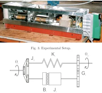
transfer function used in analysis is only an approximation to the actual plant dynamics. Here the (rotary) electro-mechanical, non-minimum phase test fa-cility shown in Figure 3 is used to assess the validity of the methods and results of this paper.

Fig. 3. Experimental Setup.

q

o

q

i

J

B

K

J

G

Fig. 4. Non-minimum phase characteristic.

The experimental test-bed has previously (see, for example, [10]) been used to evaluate a number of ILC schemes and consists of a rotary mechanical system of inertias, dampers, torsional springs, a timing belt, pulleys and gears.

The non-minimum phase characteristic is achieved by using the arrangement shown in Figure 4 where θi and θo are the input and output positions, Jr and

Jg are inertias,Br is a damper, Kr is a spring and Gr represents the gearing.

A further spring-mass-damper system is connected to the input in order to increase the relative degree and complexity of the system. Frequency response test measurements have been used to obtain continuous-time plant transfer-function (including a proportional plus integral plus derivative stabilizer)

G(s) = 165.95(4−s)

s4 _{+ 21.5s}3_{+ 170.28s}2_{+ 368.52s+ 663.82} (45)

hence spanned by the single vector e−4t_{. Choosing a time interval t ∈ [0,6],}

the factor αz= 4×6 = 24 so e−αz _=e−24 _{is extremely small suggesting that}

the theoretical results of this paper should apply with good accuracy.

To show the close agreement existing between predicted and measured results, 40 trials of NOILC, using cost function weights Q = 5, and R = 1, and a sampling frequency of 250Hz, have been performed, using the reference, r(t), shown in Figure 5d). The reference comprises a sinusoidal positional movement (in radians), which is both preceded and followed by periods where it is set at zero. Following the discussion under (1) and (2) at the end of Section 4, there exists a time interval for this case [0,1.5]⊂[0,6] where the referencer is zero and the plant has zero initial conditions. Hence the error e0 will be zero in

this interval leading to a low predicted final error, e∞, and associated norm ke∞k. These predicted values are shown in Figure 5a) and b) respectively, and accurately match the experimental results obtained.

0 1 2 3 4 5 6

−4 −2 0 2 Time (s) Error, e k

Predicted e_∞

0 10 20 30 40

0 2 4 6

Trial, k

Error norm, ||e

k

||

Predicted ||e_∞||

0 1 2 3 4 5 6

−10 −5 0 5 10 Time (s)

Control input, u

k

0 1 2 3 4 5 6

−5 0 5 Time (s) Output, y k

r(t) k = 2 k = 4 k = 10 k = 40

a) b)

c) d)

Fig. 5. Experimental results with initial zero period: a) error, ek, b) error norm,

kekk, c) control input, uk and d) output,yk

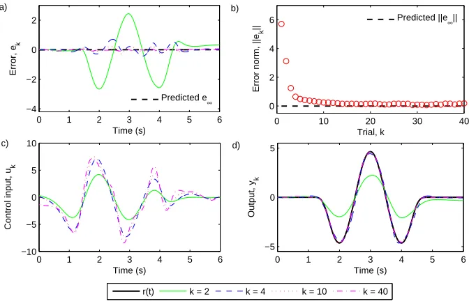
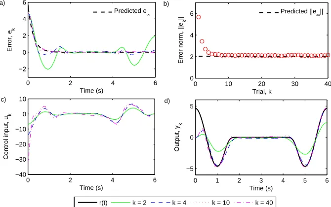
In order to examine a case where a significant non-zero final error is predicted, the reference is now replaced with that shown in Figure 6d). This corresponds to the same movement as the previous reference, however the starting point has now been changed to half way along its length. The initial period of r(t) is now not zero so, recalling again the discussion under (1) and (2) at the end of Section 4, thee0 willnotbe small in this interval, leading to predicted error

values significantly different from zero, as shown in Figure 6 a) and b). Again, 40 trials of NOILC, using cost function weightsQ= 5,and R = 1, have been performed, and the experimental error results, ek and kekk obtained can be

the predicted error is modeled by e∞≈6e−4t _{(plot a) in Figure 6).}

0 2 4 6

−2 0 2 4 6 Time (s) Error, e k

Predicted e_∞

0 10 20 30 40

0 2 4 6

Trial, k

Error norm, ||e

k

||

Predicted ||e_∞||

0 2 4 6

−40 −30 −20 −10 0 10 Time (s)

Control input, u

k

0 1 2 3 4 5 6

−5 0 5 Time (s) Output, y k

r(t) k = 2 k = 4 k = 10 k = 40

a) b)

c) _d)

Fig. 6. Experimental results without initial zero period: a) error,ek, b) error norm,

kekk, c) control input, uk and d) output,yk

6 Conclusions

The paper has modeled observed behavior of norm optimal iterative learning control when the plant has a number of open right-half plane zeros. This ob-served behavior consists of two phases of convergence. The first occurs in the first few iterations where the algorithm normally exhibits good (and poten-tially rapid) error norm reductions. The second phase then sets in and exhibits extremely slow reductions, typically so slow that, to all practical intents and purposes, the algorithm is not converging. The plot of ||ek|| against k

ap-pears to ”plateau” at a constant value that represents the best experimental accuracy that can be achieved.

This phenomenon has been explained by proving that the self-adjoint plant operator GG∗ _{almost annihilates well-defined signals associated with the} ze-ros e.g. one such signal for a zero z is e−zt_{. The span of these signals is an}

m−dimensional subspace E+ of the output signal space where convergence is

inevitably slow. In contrast, convergence of the component in the orthogonal complement E⊥

+ can be rapid.

using Lagrangian methods. The model provides some insight into the effects of initial error e0 and reference signal on the algorithm behavior and suggests

that a small initial error and/or a reference signal with an initial period of inactivity are simple practical ways of improving performance and accuracy. Finally the predictions of the model have been shown to be good in practice using an electro-mechanical benchmarking experiment.

Further work is needed to generalize the ideas to the case of input multi-output systems (where the same phenomenon occurs).

References

[1] Arimoto, S., Kawamura, S. & Miyazaki, F., Bettering operations of robots by learning, 1984, Journal of Robotic Systems, 1, pp. 123–140.

[2] Bristow, D. A., Tharayil, M., & Alleyne, A. G., A survey of iterative learning control, IEEE Control Systems Magazine, 2006, 26(3), pp. 96–114.

[3] Ahn, H.-S., Chen, Y., and Moore, K. L., Iterative learning control: brief survey and categorization, 2007, IEEE Transactions on Systems, Man and Cybernetics, Part. C, 37(6), pp. 1109–1121.

[4] N. Amann & D. H. Owens Non-minimum phase plants in iterative learning control, Proc International Conference on Intelligent Systems Engineering, IEE Conf Publication No 395, pp. 107–112, 1994.

[5] Amann, N., Owens, D. H. & Rogers, E.,Iterative learning control using optimal feedback and feedforward actions, 1996, International Journal of Control, 65(2), pp. 277–293.

[6] Owens, D. H., Hatonen, J.J. & Daley S., Robust monotone gradient-based discrete-time iterative learning control, 2008, International Journal of Robust and Nonlinear Control, 19, pp. 634–661.

[7] Owens, D. H. & Hatonen,Iterative learning control - An optimization paradigm, 2005, IFAC Annual reviews in Control, 29, pp. 57–70.

[8] Daley, S., Owens, D. H. & Hatonen, J,Application of optimal iterative learning control to the dynamic testing of structures, 2007, Special Issue of the Proceedings of the Institution of Mechanical Engineers, Part I (special issue on ”Dynamic Testing), 221, pp. 211–222.

[9] Kwakernakk, H. & Sivan, R. Kwakernaak, H., Sivan, R.,Linear Optimal Control Systems, Willey, New York, 1972.

[11] Ratcliffe, J.D., Lewin, P. L., Rogers, E., Hatonen J.J. & Owens, D.H.,

Norm-optimal iterative learning control applied to gantry robots for automation applications, 2006, IEEE Transactions on Robotics, 22(6), pp. 1303–1307.

[12] Kirchhoff, S., Schmidt, C., Lichtenberg, G. & Werner, H.,An iterative learning algorithm for control of an accelerator based free electron laser, 2008, Proceeding of the 47th_{IEEE Conference on Decision and Control, Cancun, Mexico, Dec 9-11,}