Evaluation of the stress singularities of plane V-notches in bonded dissimilar materials

http://eprints.whiterose.ac.uk/4916/

Article:

Niu, Z., Ge, D., Cheng, C. et al. (2 more authors) (2009) Evaluation of the stress

singularities of plane V-notches in bonded dissimilar materials. Applied Mathematical

Modelling, 33 (3). pp. 1776-1792. ISSN 0307-904X

https://doi.org/10.1016/j.apm.2008.03.007

eprints@whiterose.ac.uk

https://eprints.whiterose.ac.uk/

Reuse

See Attached

Takedown

If you consider content in White Rose Research Online to be in breach of UK law, please notify us by

Other uses, including reproduction and distribution, or selling or

licensing copies, or posting to personal, institutional or third party

websites are prohibited.

In most cases authors are permitted to post their version of the

article (e.g. in Word or Tex form) to their personal website or

institutional repository. Authors requiring further information

regarding Elsevier’s archiving and manuscript policies are

encouraged to visit:

Evaluation of the stress singularities of plane V-notches in bonded

dissimilar materials

Zhongrong Niu

_{, Dali Ge}

_{, Changzheng Cheng}

_{, Jianqiao Ye}

_{, Naman Recho}

a_{School of Civil Engineering, Hefei University of Technology, Hefei 230009, PR China} b_{School of Civil Engineering, The University of Leeds, Leeds LS2 9JT, UK}

c

Institute JLRA – CNRS UMR 7190, University P. and M. Curie-Paris VI, 75005 Paris, France

a r t i c l e i n f o

Article history:

Received 27 July 2007

Received in revised form 16 March 2008 Accepted 25 March 2008

Available online 1 April 2008

Keywords:

Stress singularity orders

Ordinary differential equations (ODEs) The interpolating matrix method V-notch

Bonded dissimilar materials Orthotropic material

a b s t r a c t

According to the linear theory of elasticity, there exists a combination of different orders of stress singularity at a V-notch tip of bonded dissimilar materials. The singularity reflects a strong stress concentration near the sharp V-notches. In this paper, a new way is proposed in order to determine the orders of singularity for two-dimensional V-notch problems. Firstly, on the basis of an asymptotic stress field in terms of radial coordinates at the V-notch tip, the governing equations of the elastic theory are transformed into an eigen-value problem of ordinary differential equations (ODEs) with respect to the circumferential coordinateharound the notch tip. Then the interpolating matrix method established by the first author is further developed to solve the general eigenvalue problem. Hence, the sin-gularity orders of the V-notch problem are determined through solving the corresponding ODEs by means of the interpolating matrix method. Meanwhile, the associated eigenvec-tors of the displacement and stress fields near the V-notches are also obtained. These func-tions are essential in calculating the amplitude of the stress field described as generalized stress intensity factors of the V-notches. The present method is also available to deal with the plane V-notch problems in bonded orthotropic multi-material. Finally, numerical examples are presented to illustrate the accuracy and the effectiveness of the method.

Ó2008 Elsevier Inc. All rights reserved.

1. Introduction

Recently, the development of the theory of fiber reinforced polymer (FRP) composite materials has been further moti-vated from strengthening and repairing various engineering structures. The cases of V-notches of bonded dissimilar mate-rials are frequently encountered in engineering applications. In such cases, there exists strong stress concentration near the sharp notch and interface end. In particular, the peak stress at the notch tip is singular according to the theory of elasticity and depends on the geometrical configuration and material properties of the notch. Fatigue failure of the structures usually occurs starting from a notch tip.

For a V-notch of homogeneous elastic body with opening angle a, as shown in Fig. 1, the singular stress field near

the V-notch tip can be expressed as a series expansion with respect to the radial coordinate in the following form

[1–6]:

rij¼Aqkr~ijðhÞ; ð1Þ

S0307-904X/$ - see front matterÓ_{2008 Elsevier Inc. All rights reserved.}

doi:10.1016/j.apm.2008.03.007

*Corresponding author. Tel.: +86 551 2901437; fax: +86 551 2902066.

E-mail address:niu-zr@hfut.edu.cn(Z. Niu).

Contents lists available atScienceDirect

Applied Mathematical Modelling

where the exponentkis called stress singularity order,r~ijðhÞare the associated eigenfunctions,Ais the coefficient of the asymptopic expansion (called the generalized stress intensity factor). To study the singularity of the isotropic elastic

V-notch, Williams[1]established the characteristic equation by using the Airy stress function method, as follows:

fðkÞ ¼ ksinbþsin_ðkbÞ ¼0; ð2_Þ

whereb= 2pa. It can be seen that the exponentkdepends on the opening anglea. The smallest real position rootsk gen-erally satisfyk2(1, 0) in the casea<p.

The two key aspects of solving a V-notch problem in linear elasticity are to determine stress singularities and then find the associated amplitudes of the stress field that usually denoted as the generalized stress intensity factors of the V-notch

tip. In a general case of V-notch, the exponentkmay be real or complex.

Various methods have been proposed to treat V-notch problems. Gross et al.[7,8]and Carpenter[9]obtained the

general-ized stress intensity factors for plane V-notch problems by a boundary collocation method. Boundary element method was also used to solve the displacement and stress fields of plane V-notch problems[10,11]. In the last decade, significant more work has been done to study V-notch problems because of an increased use of coatings and composite structures. Using Eq.

(2)as a starting point, the sub-region accelerated Müller method[12]was utilized to compute the eigenvalues of the stress field near V-notch tips. The algebraic equation system in terms of unknown parameters in the analytical expression of the stress field was derived by the sub-region mixed energy principle, by which the stress amplitudes were also calculated. Jian

et al.[13]evaluated the stress exponents of V-notches made of bonded bimaterial, using a complex potential theory and

Newton’s iteration method. The stress amplitudes were then obtained in conjunction with the use of hybrid finite element.

Gadi et al. [14] derived the analytical formulations of thermally induced logarithmic stress singularities in a composite

wedge composed of incompressible materials. Through using the state space method for a plane notch formed from several bonded anisotropic materials, Li et al.[15]established a governing eigenequation according to the elasticity theory, which can provide the stress singularity orders of the V-notches by means of an iteration technique for roots finding. By applying the Lekhnitskii formalism and Stroh formalism[16], Ting[17]studied the solutions of the stress fields of general anisotropic elastic materials and composites, in which the explicit expressions of the stress functions of some cases were presented as the form of a sextic equation. With the same way, the study of stress singularities at the tip of a V-notch that consists of an arbitrary number of dissimilar anisotropic elastic wedges was given by Ting[18]. After then, Hwu et al.[19]deduced an ex-plicit closed-form eigenequation for determining the singular order near the anisotropic elastic composite wedge apex. Since the singular orderskappear in the eigenequation as some nonlinear forms, an iteration technique should be needed to search the solutions of the singular orders from the associated determinant of the eigenequation for general V-notch problems.

With the solutions of stress singularities, Labossiere and Dunn[20]and Hwu and Kuo[21] computed the stress intensity

factors through the near tip displacement and stress fields from the conventional finite element analysis as well as the cal-culation of the path-independentH-integral[22]. Chue and Liu[23], Wigger and Becker[24]obtained the eigenequations of the plane anisotropic wedges by using Lekhnitskii’s complex function method, which were used to calculate the stress

sin-gularity orders. Sue et al.[25]used complex potential function and eigenfunction expansion method to determine the stress

singularity order of a magnetoelectroelastic bonded antiplane wedge.

The above mentioned research works are difficult to find the associated eigenfunctions~rijðhÞrelated to multiple singular-ity orders of the V-notches. It is naturally considered that the conventional finite element method and boundary element method can model the singular stress field by increasing the mesh density in the notch tip region. Unfortunately, the improvement on the accuracy of the approaches is very limited in comparison with increasing a large amount of the com-putation time. Recently, a special finite element method was used to deal with some V-notch problems based on the assump-tion of asymptotic expansion of the stress field near V-notch tips. For the V-notch and line crack shown inFig. 1, Seweryn

[26]taken two or three leading terms of the asymptotic expansion in Eq.(1)as the analytical constrains of stress field in the notch tip region. Then the analytical elements are applied in order to model the stress field in the core region around the singular tip. The remaining area of the structure can be modeled using the conventional finite elements. The approach can provide two or three singular exponents and stress amplitudes. It should be noted that the way need to know the ana-lytical constrains like~rijðhÞin Eq.(1)before evaluating the singular exponent and stress field around the notch tip. Three leading terms of the analytical constrains were found only in the case of homogeneous isotropic crack[2]. However, the ana-lytical constrains are difficult to be found prior to the evaluation of the stress singularity order of general V-notch problems of bonded dissimilar multi-material. Hence some approximate constrain functions~rijðhÞare proposed to support the way.

α

ρ

θ

According to the idea, Carpinteri et al.[27]calculated the first leading singular exponent and mode I stress amplitude for the multi-layered beam with a crack or re-entrant corner symmetrically meeting a bimaterial interface with the finite element

method. Chen and Sze[3]proposed a new eigenanalysis method with hybrid finite element and the assumption of

asymp-totic expansion to determine the stress exponents and stress amplitudes of bonded bimaterial V-notches.

The aim of this paper is to study the stress singularities of plane V-notch problems of bonded dissimilar materials. The governing equations of linear elasticity are transformed to eigenvalue problems of ordinary differential equations (ODEs)

based on the assumption that the stress fields are asymptotic near the V-notch tips. The first author[28] established the

interpolating matrix method to solve two-point boundary value problems of ODEs. The method is further developed in the present work to analyze eigenvalue problems of ODEs. As an application, the stress singularity orders and the associated eigenvectors are obtained by applying the interpolating matrix method to the ODEs of V-notches.

2. The eigenvalue problems of ODEs for plane V-notches in linear elasticity

Firstly, let us consider a V-notch of isotropic material with opening angle 2ph1h2as shown inFig. 2. Define a polar

coordinate system (q,h), taking the notch tip as origin. In the linearly elastic analysis, it has been verified that the displace-ment field in the notch tip region can be expressed as a series expansion with respect to the radial coordinateqoriginating from the notch tip[4]. One typical term of the series can be written in the following form:

uqðq;hÞ ¼qkþ1u~qðhÞ; ð3aÞ

uhðq;hÞ ¼qkþ1~uhðhÞ; ð3bÞ

wherek;_u~_qðhÞand~_{uhðhÞare eigenpairs. IntroducingEq. (3)into the strain–displacement relations of linearly elastic theory} yields the strain components as

eqq¼ ð1þkÞqk~uqðhÞ; ð4aÞ

ehh¼qk~uqðhÞ þqk~u0hðhÞ; ð4bÞ

cqh¼qk~u0qðhÞ þkq k_~u

hðhÞ; ð4cÞ

where ( )0_{=d( )/dh. From linearly elastic behavior law (Hooke’s law) of plane stress problems, the plane stresses are}

ex-pressed as

rqq¼

E 1m2q

k_½ð1þkÞ~u

qþmu~qþm~u0h; ð5aÞ

rhh¼

E 1m2q

k

½ð1_þk_Þm~_uqþu~_qþ~_u0

h; ð5bÞ

rqh¼

E 2_ð1_þm_Þq

k

ðk~_uhþ~_u0

qÞ; ð5cÞ

whereEis Young’s modulus andm, Poisson’s ratio. Notice that the eigenpairs inEq. (3)depend on the configurations (wedge angles), material properties and boundary conditions of the V-notches, which are not influenced by any load. Thus the body forces are neglected and then the equilibrium equations are

o_rqq o_q þ

1 q

o_rqh o_h þ

rqqrhh

q ¼0; ð6aÞ

1 q

orhh

o_h þ orqh

o_q þ 2rqh

q ¼0: ð6bÞ

SubstitutingEq. (5)intoEq. (6)gives

~ u00

qþ

1_þm

1mk2

~ u0

hþ

2

1mkðkþ2Þu~q¼0; h2 ðh1;h2Þ; ð7aÞ

~ u00

hþ 2þ

1 2ð1þmÞk

~ u0

qþ

1

2ð1mÞkðkþ2Þu~h¼0; h2 ðh1;h2Þ: ð7bÞ

o

ρ

1

θ

θ

θ

Γ

1

Γ

Assume that all the tractions on the two edges,C1andC2, near the notch tip are zero. That is

rhh

rqh

h¼h1

¼ rhh

rqh

h¼h2

¼ 0₀

: _ð8_Þ

Hence, substitution ofEq. (5)into Eq.(8)yields

~ u0

hþ ð1þmþmkÞ~uq¼0; h¼h1 andh2; ð9aÞ

~ u0

qþk~uh¼0; h¼h1andh2: ð9bÞ

Considering that the appearance ofk2inEq. (7)leads to nonlinear eigenanalysis ifEq. (7)is directly solved, an alternative approach is adopted in this paper to transfer the equation into a linear eigenvalue problem. To this end, two new field vari-ables are introduced as follows:

g_qðh_{Þ ¼}k_u~

qðhÞ; h2 ðh1;h2Þ; ð10aÞ

ghðhÞ ¼k~uhðhÞ; h2 ðh1;h2Þ: ð10bÞ

Thus,Eq. (10),Eq. (7)can been rewritten as

~ u00

qþ

1_þm

1mk2

~ u0

hþ

2

1mðkþ2Þgq¼0; h2 ðh1;h2Þ; ð11aÞ

~ u00

hþ 2þ

1 2ð1þmÞk

~ u0

qþ

1

2ð1mÞðkþ2Þgh¼0; h2 ðh1;h2Þ: ð11bÞ

By following the above procedure, the evaluation of the singularity orders near a V-notch tip is transformed to solving a

lin-ear eigenvalue problem of the ODEs governed byEqs. (10) and (11)subjected to the boundary condition ofEq. (9). In the

solutions the associated eigenfunctions~_uqand~_{uhcan also be obtained and can be used to determine the stresses in the} vicin-ity of the notch tip.

3. Evaluation of the stress singularities of V-notches of bonded dissimilar materials

Consider a V-notch problem of bonded bimaterial, as seen inFig. 3. The body consists of two subdomains of different

materials.E1andm1are, respectively, Young’s modulus and Poisson’s ratio of subdomainX1, andE2andm2are ones of

sub-domainX2. From the above derivation, it is obvious thatEqs. (10) and (11)are valid for each subdomain for analyzing the

stress singularity orders near the interface tip of the dissimilar materials. Thus, the respective governing equations in the two subdomains are written as

~ u00

1qþ

1_þm1

1m1

k2

~ u0

1hþ

2 1m1ð

k_þ2_Þg_1q¼0; h_{2 ð}h1;h2Þ; ð12aÞ

~ u00

1hþ 2þ

1

2ð1þm1Þk

~ u0

1qþ

1

2ð1m1Þðkþ2Þg1h¼0; h2 ðh1;h2Þ; ð12bÞ

g1qðhÞ ¼ku~1qðhÞ; h2 ðh1;h2Þ; ð13aÞ

g₁hðhÞ ¼k~u1hðhÞ; h2 ðh1;h2Þ ð13bÞ

and

~ u00

2qþ

1_þm2

1m2

k2

~ u0

2hþ

2 1m2ð

k_þ2_Þg_2q¼0; h_{2 ð}h2;h3Þ; ð14aÞ

~ u00

2hþ 2þ

1

2ð1þm2Þk

~ u0

2qþ

1

2ð1m2Þðkþ2Þg2h¼0; h2 ðh2;h3Þ; ð14bÞ

o

ρ

θ

θ

θ

Γ

Γ

θ

Ω

Ω

Γ

g₂qðhÞ ¼ku~2qðhÞ; h2 ðh2;h3Þ; ð15aÞ

g_2hðh_{Þ ¼}k~_{u2hðhÞ; h2 ðh2;h3Þ; ð15bÞ}

whereu~1qðhÞ;~u1hðhÞare the eigenfunctions of displacement components in subdomainX1near the notch tip;~u2qðhÞ;u~2hðhÞare

the corresponding functions in subdomainX2. For the bonded bimaterial, the continuity conditions of displacement

compo-nents and the interface tractions must be satisfied onC2, i.e.,

~

u1qðh2Þ ¼~u2qðh2Þ; ð16aÞ

~

u1hðh2Þ ¼u~2hðh2Þ ð16bÞ

and

r1hh

r1qh

h¼h2

¼ r2hh

r2qh

h¼h2

: _ð17Þ

Substitution ofEq. (5)into Eq.(17)gives

E1

1m2 1

½~_u0

1hþ ð1þm1þm1kÞ~u1q

E2

1m2 2

½~_u0

2hþ ð1þm2þm2kÞu~2q ¼0; h¼h2; ð18aÞ

E1

2_ð1_þm1Þð

~ u0

1qþk~u1hÞ

E2

2_ð1_þm2Þð

~ u0

2qþk~u2hÞ ¼0; h¼h2: ð18bÞ

Similar toEq. (9), applying the traction-free boundary conditions onC1andC3yields

~ u0

1hþ ð1þm1þm1kÞu~1q¼0; h¼h1; ð19aÞ

~ u0

1qþk~u1h¼0; h¼h1; ð19bÞ

~ u0

2hþ ð1þm2þm2kÞu~2q¼0; h¼h3; ð20aÞ

~ u0

2qþk~u2h¼0; h¼h3: ð20bÞ

Thus, the evaluation of the singularity ordersknear the V-notch tip of bonded bimaterial has been transformed into solving ODEsEqs. (12)–(15)subjected to boundary conditionsEqs. (16), (18)–(20).

4. Evaluation of the stress singularities of V-notches of orthotropic materials

Consider a plane V-notch problem of orthotropic material, as seen inFig. 4. Two principal axes of the orthotropic material are denoted Axes 1 and 2, respectively.h0is the angle between Axis 1 andx-direction of the Cartesian coordinate systemoxy.

oqhis a polar coordinate system where the notch tip is the pole.E11andE22are the elastic moduli of the orthotropic material

in 1-direction and 2-direction, respectively,G12is the shear modulus, andm12is Poisson’s ratio.

In the same way, the displacement field,Eq. (3), in the notch tip region is also acceptable for the plane V-notch problem of orthotropic material.

In the polar coordinate systemoqh, the strain–stress relationships can be written as

rqq rhh rqh 8 > < > : 9 > = > ; ¼

D11 D12 D16

D12 D22 D26

D16 D26 D66

2 6 4 3 7 5 eqq ehh eqh 8 > < > : 9 > = > ;

; ð21_Þ

o

ρ

θ

θ

θ

Γ

Γ

θ

x

where

D11¼

p₁cos4_{ðhÞ þp}

2sin 4

ðhÞ þ2 cos2_ðhÞsin2

ðhÞð2G12p3þp4Þ

p3

;

D12¼

p_4ðcos4_{ðhÞ þsin}4

ðh_{ÞÞ þ}cos2_ðhÞsin2

ðh_Þðp_1þp₂4G12p3Þ

p₃ ;

D16¼cosðhÞsinðhÞ

p1cos2ðhÞ p2sin 4

ðhÞ þ ðsin2_{ðhÞ cos}2_ðhÞÞð2G

12p3þp4Þ

p₃ ;

D22¼

p2cos4ðhÞ þp1sin 4

ðhÞ þ2 cos2_ðhÞsin2

ðhÞð2G12p3þp4Þ

p3

;

D26¼cosðhÞsinðhÞ

p₁sin2_ðh_Þ p₂cos4_{ðhÞ ðsin}2

ðh_Þ cos2_ðhÞÞð2G

12p3þp4Þ

p₃ ;

D66¼

G12p3ð14 cos2ðhÞsin 2

ðh_{ÞÞ þ}sin2_ðh_Þcos2_ðhÞðp

1þp22p4Þ

p₃ ;

h¼h0h:

ð22Þ

For the plane stress problem, there are

p_1¼ E2

11; p2¼ E11E22; p3¼t212E22E11; p4¼t12E11E22: ð23Þ

Substitution of Eq.(4)into Eq.(21)yields the stress components as

rqq¼qk½D16~u0qðhÞ þD12~u0hðhÞ þ ðD11þD12Þu~qðhÞ þkðD11u~qðhÞ þD16u~hðhÞÞ; ð24aÞ

rhh¼qk½D26~u0qðhÞ þD22~u0hðhÞ þ ðD12þD22Þu~qðhÞ þkðD12u~qðhÞ þD26u~hðhÞÞ; ð24bÞ

rqh¼qk½D66u~0qðhÞ þD26u~0hðhÞ þ ðD16þD26Þ~uqðhÞ þkðD16~uqðhÞ þD66~uhðhÞÞ: ð24cÞ

According to the same derivations as Section2, by substitutingEq. (24)into the equilibrium equationsEq. (6)and introduc-ing the two field variablesgq(h) andgh(h), one can obtain the ODE of the plane V-notch problems of orthotropic material as

follows:

g_q¼k~_{uq; h2 ½h1;h2; ð25aÞ}

g_h¼k~_u

h; h2 ½h1;h2; ð25bÞ

D66~u00qþD26~u00hþ2D16u~0qþ ðD12D22Þu~0hþ ðD11D22Þ~uqþk½2D16~u0qþ ðD12þD66Þ~u0hþ2D11u~q

þ ðD16D26Þ~uh þk½D11gqþD16gh ¼0; h2 ½h1;h2; ð25cÞ

D26~u00qþD22~u00hþ ðD12þD22þ2D66Þu~0qþ2D26~u0hþ2ðD16þD26Þu~qþk½ðD12þD66Þu~0q

þ2D26u~0hþ ð3D16þD26Þ~uqþ2D66~uh þk½D16gqþD66gh ¼0; h2 ½h1;h2: ð25dÞ

If the traction-free surfaces onC1andC2are assumed, introduction ofEq. (24)into Eq.(8)results in the boundary

con-ditions related to the ODEEq. (25)as follows:

D26~u0qþD22~uh0 þ ðD12þD22Þu~qþk½D12~uqþD26u~h ¼0; h¼h1 andh2; ð26aÞ

D66~u0qþD26~uh0 þ ðD16þD26Þu~qþk½D16~uqþD66u~h ¼0; h¼h1 andh2: ð26bÞ

If the V-notch is fixed surface onC1orC2, the boundary condition can easily be expressed as

~

uq¼0; h¼h1orh2; ð26cÞ

~

uh¼0; h¼h1 orh2: ð26dÞ

Hence, the evaluation of the singularity orderskand the associated eigenfunctions~_uqand_u~_hnear the V-notch tip of

ortho-tropic material has been also transformed into solving ODEsEq. (25)subjected to boundary conditionsEq. (26).

Furthermore, for the solutions of plane V-notch problems of bonded dissimilar multi-material, including the orthotropic materials and anisotropic materials, the same deduction process as shown above can be implemented to compute eigenso-lutions of the associated ODEs, by which the stress singularity near the V-notch is then determined. This process will produce a set of ODEs that are similar toEqs. (14)–(16), (18), (20), (25) and (26).

In order to find the solution of the ODEs derived above, in what follows, a numerical method is presented to solve the eigenvalue problems of the ODEs.

5. Interpolating matrix method for solving eigenvalue problems of ODEs

With the development of modern computer techniques, numerical methods have been proposed to solve two-point boundary value problems (BVPs) of ODEs. At present, the most commonly used methods for solving ODEs are the finite dif-ference, shooting and collocation methods. On the basis of the above algorithms, several general-purpose computer routines

have been designed as solvers of the BVPs of ODEs. These solvers include PASVA, BOUNDS, SUPORT[29]and COLSYS[30]. The

the highest derivative appearing in the ODEs is chosen as the unknown parameter of the discrete ODE system. In general, most of the existing methods, including the above mentioned ones, have their own merits and are complementary, depend-ing on the nature of the problems to be solved. However, most of the above solvers deal with two-point BVPs only. To solve the V-notch problems, an efficient method to deal with eigenvalue problems of ODEs is apparently needed. In the present paper, the interpolating matrix method is further developed to solve the above mentioned eigenvalue problems.

Let us consider a set of general linear ODEs, as shown below:

Xr

k_¼1

Xmk

j_¼0

gikjðxÞyð jÞ kðxÞ k

Xr

k_¼1

Xmk

j_¼0

qikjðxÞyð jÞ

k ðxÞ ¼fiðxÞ; i¼1ð1Þr; x2 ½a;b ð27Þ

subjected to the following boundary conditions:

Xr

k¼1

X mk1

j¼0

alkjyð j_Þ

kðnlkjÞ k Xr

k¼1

X mk1

j¼0

blkjyð j_Þ

kðnlkjÞ ¼cl; l¼1ð1Þt; a6nlkj6b; ð28Þ

where the symbol 1(1)rdenotes 1, 2,. . .,r;fi(x),gikj(x) andqikj(x)2c0[a,b] are known functions with respect tox;mkstands for the highest order of the derivative of each undetermined functionyk(x) in Eq.(27);yð

jÞ

k stands for thejth order derivative of the functionyk(x);t¼P

r

k_¼1mkis the number of the boundary conditions Eq.(28);alkj,blkjandclare known real scalars.nlkj can be arbitrary values in the interval [a,b], which express that Eq.(28)can be multi-point boundary conditions. Notice that whenfi(x) andclare identically zero, Eqs.(27) and (28)form an eigenvalue problem of the ODEs, wherekis the associated eigen-parameter.

The interval [a,b] is divided intonsubintervals at divisionsa=x0,x1,. . .,xn=b. Lethi=xixi1be the length of theith

sub-interval. Applying Eq.(27)at each of the divisionsxi, (i= 0, 1,. . .,n), results in

Xr

k_¼1

Xmk

j_¼0

GikjYð jÞ kðxÞ k

Xr

k_¼1

Xmk

j_¼0

QikjYð jÞ

kðxÞ ¼0; i¼1ð1Þr; ð29Þ

where

Gikj¼diagðgikjðx0Þ;gikjðx1Þ;. . .;gikjðxnÞÞ;

Qikj¼diagðqikjðx0Þ;qikjðx1Þ;. . .;qikjðxnÞÞ;

Yð_kjÞ_ðx_{Þ ¼ ð}yj_kðx0Þ;yjkðx1Þ;. . .;y j

kðxnÞÞT; k¼1ð1Þr; j¼0ð1Þmk: Letyðj_Þ

ki denote the approximate values ofyð j_Þ

kðxÞatxi,i= 1(1)n. The well-known finite difference method takesykiat the

divi-sionsxias the basic unknowns of the algebraic equations of the discrete system. Instead, the interpolating matrix method

takesyk0;y0k0;. . .;yð

mk1Þ k0 ;yð

mkÞ k0 ;yð

mkÞ

k1 ;. . .;yð

mkÞ

kn ðk¼1ð1ÞrÞas the basic unknowns after discretization. As a result, the (j1)th or-der or-derivative ofyk(x) can be expressed in terms of itsjth order derivative based on the following integration:

yð_kj1Þ_ðxiÞ yð j1Þ k ðx0Þ ¼

Z x_i

x₀

yð_kjÞ_ðx_Þdx;j_¼1_ð1_Þmk;k¼1ð1Þr;i¼1ð1Þn: ð30Þ

Within interval [a,b],yðj_Þ

k ðxÞcan be approximated with the piecewise polynomial interpolation as

yðj_Þ kðxÞ ¼

Xn

i_¼0

yðj_Þ

kðxiÞLiðxÞ þdð j_Þ

knðxÞ; x2 ½a;b; ð31Þ

where Li(x) are the Lagrangian interpolation polynomials and dðknjÞðxÞ are the residual errors. Introduce the following notations:

xli¼ Z x_l

x₀

LiðxÞdx; i;l¼0ð1Þn; ð32aÞ

Ykðx0Þ ¼ ðykðx0Þ;y0kðx0Þ;. . .;yðkmk1Þðx0ÞÞ

T_{; Y}

k0¼ ðyk0;y0k0;. . .;yð

mk1Þ k0 Þ

T_;

Y_kðjÞ¼ ðyð_kj₀Þ;y_kðj₁Þ;. . .;y_knðjÞÞT; r¼ ð1;1;. . .;1ÞT_ðn_þ1Þ; ð32bÞ

Rð_kljÞ¼

Z x_l

x₀

d_knðjÞðxÞdx; Rð_kjÞ¼ ðR_kðj₀Þ;Rð_kj₁Þ;. . .;Rð_knjÞÞT: ð32cÞ

Substituting Eq.(31)into(30), and calculating the integrals fori= 0, 1,. . .,n, one obtains

Yðj1Þ k ðxÞ ¼yð

j1Þ

k ðx0ÞrþDYðjÞ kðxÞ þRð

j_Þ

k; x2 ½a;b: ð33Þ

In Eq.(33),D= [xli] is an (n+ 1)(n+ 1) matrix whose elements are calculated from the integral in Eq.(32a)and, therefore, calledintegral matrix. For the piecewise linear interpolation, the basis functions in Eq.(31)are

LiðxÞ ¼

ðxxi1Þ=hi; x2 ½xi1;xi;

ðxxiþ1Þ=hiþ1; x2 ½xi;xiþ1;

0; others:

8 > <

> :

Substituting Eq.(34a)into Eq.(32a)and calculating the integralsxli, (i,l= 0(1)n), we gain the integral matrix with the linear interpolation which can be written as

D¼0:5

0 0 0 0

1 1 0 0

.. . .. . . . . .. .

1 1 1 0

1 1 1 1

2 6 6 6 6 6 6 4 3 7 7 7 7 7 7 5

0 0 0 h1 h1 ..

.

0

0 h2 h2 . .

. .. . .. . . . . . . . . . . 0

0 0 hn hn

2 6 6 6 6 6 6 6 6 4 3 7 7 7 7 7 7 7 7 5

ðn_þ1Þðn_þ1Þ

ð34b_Þ

Thus, for an arbitraryj, the recurrence relation of Eq.(33)results in

YðkjÞðxÞ ¼PkjYkðx0Þ þDmkjYðkmkÞðxÞ þrð jÞ

k; k¼1ð1Þr; j¼1ð1Þðmk1Þ; ð35Þ

where

rðj_Þ k ¼

X mk1j

l¼0

½Dl_Rðj_þ1þl_Þ

k ð36Þ

are the local truncated errors ofYð_kjÞ_ðx_Þ, and

Pkj¼ ½0;. . .;0

zfflfflfflffl}|fflfflfflffl{ j

;r;Dr;. . .;Dmk1jr

ðnþ1Þm_k ð37Þ

is an (n+ 1)mkmatrix. Ignoringrð jÞ

k in Eq.(35)yields

Yðj_Þ

k ¼PkjYk0þDmkjYð

m_kÞ

k ; k¼1ð1Þr; j¼1ð1Þðmk1Þ: ð38Þ

It can be seen from Eq.(38)thatYðj_Þ

k have been represented byYk0andYð

m_kÞ

k . Substituting Eq.(38)into Eq.(29)gives the fol-lowing algebraic equations:

Xr

k¼1

½AikYk0þBikYð m_kÞ

k k

Xr

k¼1

½AkikYk0þBkikYð m_kÞ

k ¼0; ð39Þ

whereAikandAkikare (n+ 1)mkmatrices;BikandBkikare (n+ 1)(n+ 1) matrices. They are, respectively

Aik¼ X m_k1

j¼0

GikjPkj; Bik¼ Xmk

j¼0

GikjD m_kj

; Akik¼ X m_k1

j¼0

QikjPkj; Bkik¼ Xmk

j¼0

QikjD m_kj

: ð40_Þ

Without loss of generality, consider that thenlkjin Eq.(28)take the interval divisions atxIlð06Il6nÞwithin [a,b]. In the

case of the so-called two-point BVPs,Iltake 0 andnwherenlkjhave the values ofaandb. Introducing Eq.(38)into Eq.(28) and lettingcl= 0 yield the following eigenvalue problem:

Xr

k¼1

X mk1

j¼0

alkj ðPkjÞIlYk0þ ðD m_kj

ÞIlY ðm_kÞ k

h i

kX

r

k¼1

X mk1

j¼0

blkj ðPkjÞIlYk0þ ðD mkj

ÞIlY ðm_kÞ k

h i

¼0; ð41_Þ

where_ðPkjÞI_landDI_ldenote theIlth row of matricesPkjandD, respectively. Introducing the following notations into Eq.(41)

Valk¼ X mk1

j_¼0

alkjðPkjÞI_l; Walk¼ X mk1

j_¼0

alkjðD m_kj

ÞI_l; ð42aÞ

Vblk¼ X mk1

j¼0

blkjðPkjÞIl; Wblk¼ X mk1

j¼0

blkjðD mkj

ÞIl; l¼1ð1Þt ð42bÞ

and rewriting the equation, one obtains

Xr

k_¼1

ðValkYk0þWalkYð mkÞ k Þ k

Xr

k_¼1

ðVblkYk0þWblkYð m_kÞ

k Þ ¼0: ð43Þ

Using the following notations:

Y0¼ Y10

Y20

.. .

Yr0

8 > > > > < > > > > : 9 > > > > = > > > > ; t

; Y_¼ Yðm_1Þ

1

Yðm_2Þ

2

.. .

Yðm_rÞ r 8 > > > > > < > > > > > : 9 > > > > > = > > > > > ;

r_ðn_þ1Þ

; t_¼X r

k_¼1

Va¼ ½Valktt; Wa¼ ½Walktr_ðn_þ1Þ; Vb¼ ½Vblktt; Wb¼ ½Wblktr_ðn_þ1Þ; k¼1ð1Þr; l¼1ð1Þt; ð45aÞ

A_{¼ ½}Aikr_ðn_þ1Þt; B¼ ½Bikr_ðn_þ1Þr_ðn_þ1Þ; Ak¼ ½Akikr_ðn_þ1Þt; Bk¼ ½Bkikr_ðn_þ1Þr_ðn_þ1Þ; i;k¼1ð1Þr ð45bÞ

and converting Eqs.(39) and (43)into a combined matrix form, we arrive finally at

Va Wa

A B

_Y

0

Y

k Vb Wb Ak Bk

_Y

0

Y

¼0: ð46_Þ

Eq.(46)is a generalized eigenequation system ofr(n+ 1) +torders in the unknowns_ðYT 0;YTÞ

T_{. It can always be converted into}

a standard eigenvalue formulation through the following transformation:

C1 2 C1

Y0

Y

k Y0 Y

¼0 or 1 k

Y0

Y

C1 1 C2

Y0

Y

¼0; ð47_Þ

where

C1¼

Va Wa

A B

; C2¼

Vb Wb

Ak Bk

: ð48_Þ

Numerical methods from various textbooks about numerical analyses are available to solve the algebraic eigenvalue equa-tions like Eq.(47). In general, the solutions of Eq.(47)provide a finite number of eigenvalues,k, and the associated eigen-vectors _ðYT₀;YTÞT. Furthermore the substitution of _ðYT₀;YTÞTinto Eq. (38) gives the eigenvectors of all the derivatives of yk(x), i.e.Yk;Y0k;. . .;Yð

mk1Þ

k ;ðk¼1ð1ÞrÞ.

It can be seen from the above deduction that the formations of the coefficient matrices in Eq.(47)rely on the integral

matrix Dbesides those known functions and parameters in ODEs(27) and (28). In the interpolating matrix method, Eq.

(46)or(47)is used to solve the eigenvalue problems of ODEs(27)with the boundary conditions(28), in which the computed error arises from the local truncated errorsrðj_Þ

k in Eq.(35). Thus the accuracy of the interpolating matrix method depends on

the integral matrix which represents the influence of a piecewise polynomial interpolation to approximateyðkjÞðxÞ. Generally, the integral matrixDwith the piecewise quadratic or spline function interpolation is encouraged because of their higher or-der approximation in comparison with the linear one.

It has been found that for analyzing two-point BVPs of ODEs, in addition to the same some merits as the finite difference and collocation methods, the interpolating matrix method has two distinct advantages as: (1) All functions and their deriv-atives appearing in the BVPs of ODEs are simultaneously obtained with the same degree of accuracy. This feature is partic-ularly beneficial to the calculation of stress field that requires the first derivative of the displacement functions. (2) It can solve the general eigenvalue problems of ODEs and be convenient to write a general-purpose routine, since the implemen-tary procedure has been expressed as the above unified formulations, especially for the boundary conditions Eq.(28). More-over, all the solutions corresponding each eigenpair are also obtained with the same degree of accuracy.

According to the above formulations, a general-purpose routine calledIMMEIis developed in FORTRAN, in which the

interpolating matrix method is adopted to solve two-point eigenvalue problem in ODEs expressed in the form of Eqs.

(27) and (28).

6. Numerical examples

6.1. Numerical example of solving eigenvalue problems

Before applying the above developed method to V-notch problems, a simple example is shown here to illustrate the effec-tiveness of the new approach.

Example 1. Bending vibration of a uniform beam hinged at both ends (Fig. 5). The free vibration equation of the beam is

d4Y_ðx_Þ

dx4 b

4_Y

ðx_{Þ ¼}0; b4_¼x

2_m

EI ; x2 ½0;L; ð49aÞ

y

L

x

whereY(x) is the natural mode of transverse displacement;xis the natural frequency;Lis the length of the beam;EIdenotes

the flexural rigidity andmthe mass per unit length. Here, bothEIandmare constant. At the two ends, the boundary

con-ditions are, respectively,

Yð0_{Þ ¼}0; Y00_{ð0Þ ¼0; YðLÞ ¼0; Y}00_{ðLÞ ¼0: ð49bÞ}

Y(x) andxare determined by solving the eigenvalue problem ofEq. (49), for which exact solutions are available and are

xi¼ ðipÞ2 ffiffiffiffiffiffiffiffiffi

EI mL4 s

; i¼1;2;. . ._{; ð}50aÞ

YiðxÞ ¼Aisin ipx

L ; ð50bÞ

whereAiare amplitudes of the mode shapes.

To assess accuracy of the interpolating matrix method (IMMEI), linear and quadratic interpolation functions are used, respectively, to compute the eigenpairs. Here the interval [0,L] is divided into three uniform meshes with the number of sub-intervals being (n=) 20, 40 and 80, respectively. The solutions of IMMEI in the three meshes are presented to show the con-vergence rate of the interpolating matrix method as the number of the divisions doubly increases.Table 1shows the relative

errors of the computed eigenvaluesxiusing IMMEI in comparison with the exact solutions. The relative errors of the

solu-tionsYiðxÞ;Y0iðxÞ;Yi00ðxÞandY000i ðxÞof the first four modes using IMMEI with the piecewise quadraticDandn= 80 are plotted in Figs. 6–9, in turn. InTable 1andFigs. 6–9, the err% means the relative error defined by below:

err%_¼solutionapproxsolutionexact

solutionexact

100: ð51_Þ

All of the eigenpairs and their derivatives of various orders ofYi(x) are simultaneously computed by IMMEI for each mesh.

Among them, the computational accuracy of the first eigensolution is highest, whose relative error is about 105_{shown in}

Table 1andFig. 6when the quadraticDwithn= 80 is chosen. The accuracy of the solutions is lost gradually for higher modes in the discrete model. Obviously, accuracy can be improved by increasing the number of the divisions of the discrete system.

Comparatively, the accuracy using the quadraticDis very higher than one using the linearDon the same number of the

divisions. Many numerical experiments have illustrated that the convergence rates of the present method are about O(h4₎

for the quadraticDand O(h2_{) for the linearD, respectively, wherehis the length of the subinterval.}

Table 1

The natural frequenciesxið ffiffiffiffiffiffiffiffiffiffiffiffiffiffiffiffi

EI=mL4

q

Þand the relative errors (%) of the IMMEI solutions

Modes Exact solutionsxi err% of IMMEI with the linearD err% of IMMEI with the quadraticD

n= 20 n= 40 n= 80 n= 20 n= 40 n= 80

First p2 _{0.4127 0.1029 0.02571 0.001356 0.0001004 0.0000068}

Second 4p2 _{1.6682 0.4127 0.1029 0.02183 0.001607 0.000108}

Third 9p2 3.8210 0.9326 0.2318 0.1116 0.008139 0.000548

Fourth 16p2 6.9676 1.6682 0.4127 0.3575 0.02574 0.001733

Fifth 25p2 11.257 2.6275 0.6461 0.8873 0.06288 0.004229

Sixth 36p2 3.8210 0.9326 1.8773 0.13050 0.008767

Seventh 49p2 5.2621 1.2730 3.5648 0.24205 0.01624

0.0 0.2 0.4 0.6 0.8 1.0

-0.000002 0.000000 0.000002 0.000004 0.000006 0.000008 0.000010 0.000012 0.000014 0.000016 0.000018

Relative errors of 1st mode

X/L Y'''(X) Y''(X) Y'(X) Y(X)

In addition, as an advantage of the present method, it can be seen inTable 1 and Figs. 6–9 that all of the solutions YiðxÞ;Y0iðxÞ;Y00iðxÞandY000iðxÞfor each mode have the same degree of accuracy as the associated natural frequency in terms of their maximum relative errors as comparisons. However, in the finite element and finite difference approaches, the accu-racy of the derivatives of higher orders of the modes is lost rapidly because of using the difference.

0.0 0.2 0.4 0.6 0.8 1.0

-0.00002 0.00000 0.00002 0.00004 0.00006 0.00008 0.00010 0.00012 0.00014 0.00016 0.00018 0.00020 0.00022 0.00024 0.00026 0.00028

Relative errors of 2nd mode

X/L Y'''(X) Y''(X) Y'(X) Y(X)

Fig. 7.The computational errors of second mode and its derivatives of higher orders,n= 80.

0.0 0.2 0.4 0.6 0.8 1.0

-0.0002 0.0000 0.0002 0.0004 0.0006 0.0008 0.0010 0.0012 0.0014 0.0016 0.0018

Relative errors of 3rd mode

X/L Y'''(X) Y''(X) Y'(X) Y(X)

Fig. 8. The computational errors of third mode and its derivatives of higher orders,n= 80.

0.0 0.2 0.4 0.6 0.8 1.0

0.000 0.001 0.002 0.003 0.004 0.005

Relative errors of 4th mode

X/L Y'''(X) Y''(X) Y'(X) Y(X)

6.2. Numerical examples of the V-notch problems

This section is concerned with the application of the interpolating matrix method (IMMEI) to the evaluation of the

sin-gularity orders of two-dimensional V-notched problems. In the following examples, the integral matrixDwith quadratic

interpolation and uniform division is used in the routine IMMEI.

Example 2. A V-notch of isotropic material as shown inFig. 2.

The study of the single isotropic V-notch is for the purpose of comparison. Using the sub-region accelerated Müller

meth-od, Fu and Long[12]computed a number of eigenvalues of the stress singularity orders of the V-notch problem. Here the

routine IMMEI (ab. IMM) is performed to solve the ODEs,(11), (10) and (9)wherem= 0.3 and the opening angleavaries from

0° to 170°. In fact, the computed eigenvalues for the V-notch of a homogeneous isotropic material are independent to

Poisson’s ratio, while the displacement eigenfunctions andmare related. For each givena, interval [h1,h2] are divided into

three uniform meshes withn= 20, 40 and 80, respectively, where the interval implies a circle arc fromh1toh2with a radius

qat the V-notch tip. The newly computed results are given inTables 2 and 3, wherenis the number of the divisions within interval [h1,h2]. The eigenvalueskare usually complex and are expressed bykk=nk+ igkwhere i¼

ffiffiffiffiffiffiffi

1

p

. Obviously, if the imaginary partgkis equal to zero,kkis real. One of the useful features of IMMEI is that all the small eigenvalues beyond

nkP1 and their eigenvectors are determined simultaneously. Notice thatkk=1 is always a four-time repeated eigenvalue for all of the two-dimensional V-notch problems. There are two different eigenvectors associated withkk=1. When the two eigenpairs associated withkk=1 are introduced intoEq. (3), it can be found that the corresponding terms inEq. (3)

rep-resent two components of the rigid translation of the structures. Thus, this special eigenvalue is not included in Tables 2

and 3. In addition, another component of the rigid translation is referred to the term ofkk= 0 inEq. (3). Table 2lists the eigenvalues related to the symmetrical displacement (mode I) eigenfunction ~_uqðhÞand Table 3lists those related to the anti-symmetrical displacement (mode II) eigenfunction~_uqðhÞ. In the casea= 60°, the results of Ref.[26]were obtained using the special FEM by means of three leading terms of the analytical constrains of the stress field, where the half of the notch structure, due to symmetry conditions, was discretized with 152 six-node triangular elements.

Table 2

The eigenvalues corresponding to the symmetrical displacement eigenfunctionu~qðhÞ

a Methods n1 g1 n2 g2 n3 g3 n4 g4

170° Ref.[12] 0.099956 0 1.001795 0 1.695232 0 3.022680 0

IMM,n= 20 0.0997671 0 1.000629 0 1.706359 0 2.972986 0 IMM,n= 40 0.099949 0 1.001733 0 1.695693 0 3.020562 0 IMM,n= 80 0.099955 0 1.001789 0 1.695286 0 3.022390 0 150° _{Ref.[12] 0.248025 0 1.106286 0.096100 2.828294 0.347177 4.547288 0.459268}

IMM,n= 20 0.247871 0 1.109776 0.087307 2.859206 0.321400 4.705928 0.308320 IMM,n= 40 0.248019 0 1.106531 0.095588 2.830449 0.345590 4.556639 0.452879 IMM,n= 80 0.248025 0 1.106303 0.0960594 2.828434 0.347070 4.547904 0.458893 120° Ref.[12] 0.384269 0 0.833549 0.252251 2.343717 0.414037 3.849458 0.506015 IMM,n= 20 0.384138 0 0.836062 0.252153 2.365450 0.414282 3.957761 0.498516 IMM,n= 40 0.384259 0 0.833734 0.252249 2.345190 0.414126 3.856164 0.506382 IMM,n= 80 0.384268 0 0.833561 0.252251 2.343817 0.414042 3.849910 0.506043 90° _{Ref.[12] 0.455516 0 0.629257 0.231251 1.971844 0.373931 3.310377 0.455494}

IMM,n= 20 0.455395 0 0.631172 0.232519 1.988336 0.383516 3.394304 0.488602 IMM,n= 40 0.455511 0 0.629323 0.231332 1.972392 0.374414 3.313047 0.457263 IMM,n= 80 0.455516 0 0.629267 0.231257 1.971920 0.373979 3.310732 0.455687 60° _{Ref.[12] 0.487779 0 0.471028 0.141853 1.677615 0.284901 2.881487 0.360496}

Ref.[26] 0.4878 0 0.4710 0.1418 1.6776 0.2849

IMM,n= 20 0.487717 0 0.471813 0.143640 1.684805 0.296623 2.924016 0.408020 IMM,n= 40 0.487775 0 0.471073 0.141991 1.678017 0.285650 2.883292 0.363632 IMM,n= 80 0.487778 0 0.471035 0.141869 1.677673 0.284994 2.881766 0.360853 30° _{Ref.[12] 0.498547 0 0.202957 0 0.490378 0 1.440492 0.114207}

IMM,n= 20 0.498472 0 0.205806 0 0.488633 0 1.445210 0.147248 IMM,n= 40 0.498540 0 0.205806 0 0.490268 0 1.440740 0.116222 IMM,n= 80 0.498546 0 0.202983 0 0.490363 0 1.440530 0.114502

10° _{Ref.[12] 0.499947 0 0.058843 0 0.499728 0 1.118823 0}

IMM,n= 20 0.499856 0 0.060933 0 0.498345 0 1.151176 0

IMM,n= 40 0.499934 0 0.059126 0 0.499521 0 1.122380 0

IMM,n= 80 0.499946 0 0.058862 0 0.499716 0 1.119061 0

0° Exact solutions 0.50000 0 0 0 0.50000 0 1.00000 0

IMM,n= 20 .499794 0 0.003578 0 0.497325 0 1.043821 0

Tables 2 and 3show that the eigenvalues obtained using the present method approach the results of Ref.[12]asn in-creases. In the tables, the two eigenvalues in the range of1 <kk< 0 forn= 40 have converged up to the fourth significant figure. It is found that there exists either one or two real eigenvalues when 06a< 180°_{for the V-notch of isotropic material.} In this study, the eigenvalues whose real parts are between1 and 0, i.e. Re(k)₂(1, 0), are the important parameters that are directly related to the singularity order of the stress field at the V-notch tip. In addition, some eigenvalues when Re(k)P0 should be also considered if the near tip stress field is determined.

The highest order of singularity is0.5 for both mode I and mode II occurring ata= 0, i.e. for a line crack. For the crack problem, all the exact eigenvalues can be predicted to be real and take1 + 0.5k,k= 0, 1, 2,. . .It is well known in the finite element analysis that the ‘‘quarter-point” element[31,32]at crack tip can efficiently model the singular stress field near the crack tip, in which the mid-side nodes near the crack tip are placed at the quarter point. In fact, the element at crack tip assumes the following stress mode:

rij¼ aij

ffiffiffi

q

p þbijþcijpffiffiffiq; ð52Þ

which coincides with the stress field related to the first three eigenvalues0.5, 0 and 0.5. However, it can be seen inTables 2 and 3that shape function Eq.(52)of the quarter-point element is no longer available to modeling the stress field near the V-notch tips of the casesa> 10°, at least, because the singularity orders here are not0.5 and 0.5.

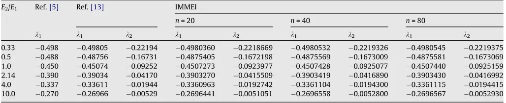
Example 3. A V-notch of bonded dissimilar bimaterial as shown inFig. 3.

The V-notch consists of two different isotropic materials and is a plane strain problem. The bonded interface lies ath=h2.

The opining angle is (h3h1). Poisson’s ratios of the materials arem1= 0.167 andm2= 0.210, respectively. In the parametric

study,E2/E1is variable. Refs.[13,5]used Newton’s iteration to calculate the stress singularities through an eigenequation

derived by using complex functions. The two intervals [h1,h2] and [h2,h3] are divided into the same number of subintervals

with equal segment in each interval. In the tables,nis the number of the divisions within each interval andkk=nk+ igkis the

same meaning toExample 2. Due to the lack of exact solutions for comparisons, very fine divisions are adopted for the

V-notch withE2/E1= 0.5,h1= 0°, h2= 90° andh3= 270°. The results using IMMEI with finer mesh of n= 160 are acted as Table 3

The eigenvalues corresponding to the anti-symmetrical displacement eigenfunction_u~ qðhÞ

a Methods n1 g1 n2 g2 n3 g3 n4 g4 n5 g5

170° _{Ref.[12] 0.798933 0 0 0 2.007826 0 2.586721 0 4.060480 0}

IMM,n= 20 0.800916 0 0 0 1.997193 0 2.631530 0 3.902388 0

IMM,n= 40 0.799004 0 0 0 2.007389 0 2.588412 0 4.048878 0

IMM,n= 80 0.798942 0 0 0 2.007772 0 2.586934 0 4.058970 0

150° _{Ref.[12] 0.485814 0 0 0 1.967836 0.261186 3.688038 0.409575 5.406179 0.500793}

IMM,n= 20 0.487279 0 0 0 1.979418 0.249763 3.760510 0.349527 5.467941 0 IMM,n= 40 0.485919 0 0 0 1.968624 0.260421 3.692685 0.406489 5.422865 0.490318 IMM,n= 80 0.485819 0 0 0 1.967891 0.261135 3.688348 0.409368 5.407307 0.500164 120° _{Ref.[12] 0.148913 0 0 0 1.589479 0.348375 3.090928 0.464641 4.601514 0.541087}

IMM,n= 20 0.150009 0 0 0 1.597549 0.348528 3.147310 0.463943 4.820487 0.503578 IMM,n= 40 0.148992 0 0 0 1.590100 0.348397 3.100330 0.464789 4.614583 0.541504 IMM,n= 80 0.148918 0 0 0 1.589517 0.348376 3.097151 0.464653 4.602357 0.541143 90° Ref.[12] 0.091471 0 0 0 1.301327 0.315838 2.641420 0.418787 3.978902 0.486625 IMM,n= 20 0.090574 0 0 0 1.307470 0.319829 2.680315 0.437987 4.148389 0.532426 IMM,n= 40 0.091436 0 0 0 1.301562 0.315956 2.642884 0.419538 3.984719 0.489385 IMM,n= 80 0.091466 0 0 0 1.301356 0.315856 2.641593 0.418888 3.979574 0.486968 60° _{Ref.[12] 0.269099 0 0 0 1.074826 0.229426 2.279767 0.326690 3.482900 0.388984}

Ref.[26] 0.2691 0 0 0 1.0749 0.2294

IMM,n= 20 0.268710 0 0 0 1.077382 0.234207 2.297998 0.351998 3.574251 0.469510 IMM,n= 40 0.269070 0 0 0 1.075014 0.229741 2.280884 0.328306 3.487289 0.394444 IMM,n= 80 0.269095 0 0 0 1.074848 0.229466 2.279900 0.326881 3.483436 0.389603 30° Ref.[12] 0.401808 0 0 0 0.838934 0 0.948560 0 1.987005 0.166741 IMM,n= 20 0.401460 0 0 0 0.881197 0 0.909578 0 1.999550 0.222443 IMM,n= 40 0.401781 0 0 0 0.840591 0 0.947180 0 1.987897 0.170364 IMM,n= 80 0.401805 0 0 0 0.839163 0 0.948357 0 1.987095 0.167222 10° _{Ref.[12] 0.470645 0 0 0 0.588609 0 0.999107 0 1.649700 0}

IMM,n= 20 0.470319 0 0 0 0.597760 0 0.991337 0 1.770116 0 IMM,n= 40 0.470599 0 0 0 0.589736 0 0.998226 0 1.659348 0

IMM,n= 80 0.470642 0 0 0 0.588685 0 0.999045 0 1.650330 0

0° _{Exact solutions 0.50000 0 0 0 0.500000 0 1.000000 0 1.50000 0}

IMM,n= 20 0.499373 0 0 0 0.513993 0 0.987129 0 1.62522 0

IMM,n= 40 0.499954 0 0 0 0.500983 0 0.999039 0 1.50741 0

the standard solution shown inTable 4. It is seen inTable 4that the first six eigenvalues yielded by takingn= 80 andn= 160

agree with each other up to the sixth significant figure. Thus, the computed results using IMMEI inTable 5are obtained by

taking up ton= 80 only. In general cases of the bimaterial V-notch of isotropic material, there exist two real eigenvalues in the range of1 <kk< 0. It can be seen inTables 4 and 5that the IMMEI solutions converge and agree well with the

alter-native numerical results. Thus, in Tables 4 and 5, the solutions of IMMEI are always given to show convergence rate of

the algorithm with respect to the division refinement and comparisons with the results from Refs.[13,5]. In general,Tables 4 and 5show that IMMEI can provide very accurate results. For instance, apart from the very small imaginary components, all the results inTable 5obtained using IMMEI withn= 40 are converged up to the fifth significant figure. Furthermore all the associated eigenvectors are computed with the same degree of accuracy.

Example 4. A plane V-notch of orthotropic material as shown inFig. 10.

The V-notch of orthotropic material is a plane stress problem. The opining angle isa. Two principal axes of the material are alongq-direction andh-direction related to the polar coordinate system, respectively.Ehh,Eqqare the hoop and radial

elas-tic moduli, respectively,lqhthe Poisson’s ratio,Gqhthe shear modulus. LetEhh/Eqq= 0.0375,Gqh/Eqq= 0.1,lqh= 0.187.

Evidently, the stress singularity orders and the stress fields near the notch roots vary as the change ofa. Delale et al.[33]

given an analytic solution for the stress singularity orders. Pageau et al.[6]used the finite element method to achieve the

numerical results for it. Here IMMEI is employed to solve the ODEsEqs. (31) and (32)in order to determine the stress

sin-gularity orders for several different opening angles. The computed results ofk1are shown inTables 6 and 7, wherenis the

number of the divisions. Notice that even if a> 180°, there exist the stress singularity orders withinki2(1, 0) for the orthotropic material. In fact, the number of the stress singularity orders within ki2(1, 0) increases as the decrease of the opening anglea. Whena= 0, the number ofkiwithin (1, 0) is maximum, where there are five stress singularity orders for the above values of the material parameters. And the first five stress singularity orders,ki, are all real roots in the case as Table 4

The eigenvalues of the V-notch withh1= 0°,h2= 90°,h3= 270°,E1/E2= 2

Methods n1 g1 n2 g2 n4 g4 n5 g5 n6 g6

Ref.[5] 0.488 0

Ref.[13] 0.48756 0 0.16731 0

IMM,n= 10 0.4873683 0 0.1663428 0 0.5784164 0.1962388 1.4616128 0.2663404 1.8648616 0.6727592 IMM,n= 20 0.4875405 0 0.1672198 0 0.5752737 0.1949118 1.4440259 0.2566424 1.8589506 0.6695227 IMM,n= 40 0.4875569 0 0.1673009 0 0.5750053 0.1948013 1.4426988 0.2558552 1.8585303 0.6692342 IMM,n= 80 0.4875581 0 0.1673069 0 0.5749855 0.1947932 1.4426019 0.2557975 1.8584998 0.6692129 IMM,n= 160 0.4875582 0 0.1673073 0 0.5749842 0.1947926 1.4425954 0.2557936 1.8584977 0.6692115

Note:n3= 0,g3= 0 for all of the above models.

Table 5

The eigenvalues of the V-notch withh1= 0°,h2= 90°,h3= 270°

E2/E1 Ref.[5] Ref.[13] IMMEI

n= 20 n= 40 n= 80

k1 k1 k2 k1 k2 k1 k2 k1 k2

0.33 0.498 0.49805 0.22194 0.4980360 0.2218669 0.4980532 0.2219326 0.4980545 0.2219375 0.5 0.488 0.48756 0.16731 0.4875405 0.1672198 0.4875569 0.1673009 0.4875581 0.1673069 1.0 0.450 0.45074 0.09252 0.4507273 0.0923977 0.4507428 0.0925077 0.4507440 0.0925159 2.14 0.390 0.39034 0.04170 0.3903270 0.0415509 0.3903419 0.0416890 0.3903430 0.0416992 4.0 0.337 0.33611 0.01944 0.3360963 0.0192742 0.3361104 0.0194300 0.3361115 0.0194415 10.0 0.270 0.26966 0.00529 0.2696441 0.0051051 0.2696558 0.0052800 0.2696567 0.0052930

θθ

E

ρρ

E

O

α

θ

shown inTable 7. InTable 6, it is seen that the computedk1using IMMEI withn= 80 are converged up to the sixth significant

figure in contrast to the results of IMMEI with n= 160 and Refs. [33,6]. In addition, all the associated eigenvectors are

achieved with the same degree of accuracy. As a result, the angular distribution functions_u~_qðhÞ,u~_hðhÞ, ~rqqðhÞ,r~hhðhÞ and ~

rqhðhÞassociated withk1whena= 180°and takingn= 80 are plotted inFigs. 11 and 12, respectively. It is seen inFig. 12that

the stress angular distribution functions using IMMEI are in good agreement with ones from Ref.[33].

Table 6

k1of the V-notch of the orthotropic material in several differenta

a IMMEI,n= 20 IMMEI,n= 40 IMMEI,n= 80 IMMEI,n= 160 Ref.[6], FEM Ref.[33], Analytic solution 240° _{0.2848977 0.2850110 0.2850194 0.2850200 0.284846 0.285032}

180° 0.6897694 0.6898106 0.6898137 0.6898139 0.689715 0.689816 120° 0.8129647 0.8129932 0.8129953 0.8129954 0.812902 0.812996 60° 0.8492186 0.8492432 0.8492450 0.8492452 0.849159 0.849246 0° 0.8555746 0.8556059 0.8556082 0.8556084 0.855492 0.855608

Table 7

The first fivekifor the V-notch of the orthotropic material whena= 0°

IMMEI,n= 20 IMMEI,n= 40 IMMEI,n= 80 IMMEI,n= 160 Ref.[6], FEM Ref.[33], Analytic solution k1 0.8555746 0.8556059 0.8556082 0.8556084 0.855607 0.855608

k2 0.8348093 0.8349901 0.8350034 0.8350043 0.834996 0.835006

k3 0.6646219 0.6655667 0.6656353 0.6656399 0.665614 0.665643

k4 0.4545949 0.4581610 0.4584159 0.4584331 0.458360 0.458441

k5 0.2141988 0.2251511 0.2259155 0.2259670 0.225788 0.225985

-1.5 -1.0 -0.5 0.0 0.5 1.0 1.5

ρ

u~

θ

u~

θ 689814

0 1=−. λ

0 30 60 90 120 150 180

Fig. 11.Displacement eigenvectors of the V-notch whena= 180°_,n= 80.

0 30 60 90 120 150 180

-1.5 -1.0 -0.5 0.0 0.5 1.0 1.5

Ref. [32] IMMEI

689814 0

1=− . λ

θ

θθ

σ~

ρρ

σ~

ρθ

σ

~