Predicting “Springback” Using 3D Surface Representation Techniques: A
Case Study in Sheet Metal Forming
S. El Salhi, F. Coenen, C. Dixon, M. S. Khan
University of Liverpool, Department of Computer Science, Ashton Building, Ashton Street, Liverpool L693BX, United Kingdom.
Abstract
Three different mechanisms are presented to allow for the representation of 3D surfaces in such a way that key features are retained while at the same time ensuring compatibility with prediction (classification) techniques. The application domain is sheet metal forming. The representations are designed to capture the nature of the surface to be manufactured and predict deformations, known as “springback”, that will occur across a surface (in a non-uniform manner) as a result of the application of a sheet steel forming process. The three representation techniques are: (i) Local Geometry Matrices (LGMs) founded on the concept of local binary patterns, (ii) Local Distance Measure (LDM) founded on the observation that the springback magnitude is affected by distance from edges and (iii) Point Series (PS) whereby local geometries are represented in terms of a linearisation. The evaluation of each of the techniques, and variations thereof, using parts that have been manufactured especially for the purpose, is fully described. The paper also reports on a statistical significance test concerning the results.
Keywords: 3D surface representation, Classification, Springback prediction
1. Introduction
The phenomena ofspringbackis a significant is-sue with respect to the sheet metal forming industry (Cafuta et al., 2012; Jeswiet et al., 2005). Spring-back is the deformation introduced into some man-ufactured part as a result of applying some forming process. As a consequence the desired shape, some prescribed 3D surface (T), is not the same as the gen-erated surface (T0), hence the quality of the manufac-tured part is compromised. The nature (magnitude and direction) of springback is related to the local geometries describing the 3D surface to be manufac-tured. If we can predict springback we can apply correcting measures to T to produce T00 so that the generated surface T0 will approximate much more closely toT. Thus given a previously manufactured
Email addresses:[email protected](S. El Salhi),[email protected](F. Coenen),
[email protected](C. Dixon),
[email protected](M. S. Khan)
part, with known springback, we wish to produce a classifier that can predict springback with respect to a particular manufacturing process (such as Asymmet-ric Incremental Sheet Forming or AISF). The chal-lenge is how best to represent the 3D surfaces of in-terest so as to facilitate the effective capture of local geometries to which individual springback dimen-sions can be related. The work presented in this pa-per is directed at exploring a number of alternative techniques for capturing the nature of 3D surfaces so as to support the effective generation of springback predictors (classifiers).
of representing local geometries in terms of a point series curve (linearisation).
The main contributions of this paper are as fol-lows.
1. A generic framework for springback predic-tion.
2. The LGM technique to represent 3D surfaces in terms oflocal geometries.
3. The LDM technique to represent 3D surfaces local geometries in terms of distances to the nearest critical features (edges or corners). 4. The PS technique to represent 3D surfaces
lo-cal geometries in terms of linearisations of points to form point series (curves).
5. Extensive comparison of the three proposed tech-niques in terms of accuracy and AUC measure-ments.
6. A statistical evaluation to identify the signifi-cant difference in operation between the use of LGM, LDM and PS in the context of 3D sur-face classification.
The operation of the three proposed techniques are compared in this paper using two flat-topped pyra-mid surfaces (shapes) which were specially manu-factured with respect to the work described (hence the degree of springback is known).
The rest of this paper is organised as follows. Section 2 presents a literature review of related work to that presented in the rest of this paper. Section 3 starts by introducing a generic framework for spring-back prediction. The three different representation techniques (LGM, LDM and PS) are then described in Sections 4, 5 and 6 respectively. The evaluation of the proposed representations, in the context of clas-sifier generation, using the two flat topped pyramid shapes is presented in Section 7. Some conclusions are presented in Section 8.
2. Related Work
In the field of 3D representation many different techniques have been proposed directed at a vari-ety of goals and objectives in the context of a range
of application domains. Example applications in-clude: (i) the translation of physical 3D surfaces into Computer Aided Graphics (CAG) formats (Hsiao & Chen, 2013; Jahanshahi & Masri, 2012), and (ii) ren-dering in the context of computer vision (Ayache, 1995; Izquierdo & Ohm, 2000) and with respect to many medical image analysis domains (Ayache, 1995; Ghanei et al., 1998; Fresno et al., 2009). Existing 3D representation techniques can be categorised accord-ing to the objective associated with the representa-tion. High level examples of such 3D object repre-sentation techniques include:
• Point Clouds: The simplest representation is a point cloud representation whereby a 3D sur-face is defined in terms of an unordered col-lection of points defined in terms of x, y, and z coordinates typically generated using either CAD software or some optical measuring tool (Alexa et al., 2001; Hoppe et al., 1992; Roth & Wibowoo, 1997).
• Range Images: Range images are 2D images depicting the distance of points in a 3D envi-ronment from a specific point, normally asso-ciated with some type of sensor device (Soucy & Laurendeau, 1995).
• Surface Representation: For 3D surface rep-resentation commonly advocated techniques in-clude: (i) mathematical techniques (implicit and parametric) (Farin et al., 2002; Munkberg et al., 2010) and (ii) mesh representations (Adams, 2013).
• Volume Representations: For volumetric data the idea of Constructive Solid Geometries (CSG) can be adopted whereby a hierarchy of boolean operations (union, difference and intersection) are applied to a collection of basic volumes so as to define more complex 3D volumes (Gold-feather et al., 1986).
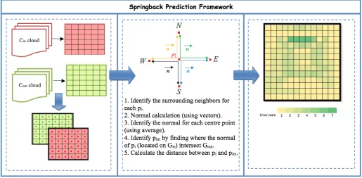
Figure 1: The process for obtaining theCin andCout 3D surface specifications.
For a more detailed discussion concerning 3D rep-resentation techniques interested readers are referred to (Hubeli & Gross, 2000) where the authors present a taxonomy of various 3D representation techniques. Classification (prediction) is the branch of ma-chine learning (knowledge discovery in data) con-cerned with the automated generation of software sys-tems that can be used to label previously unseen data. Classification is a supervised learning technique in the sense that it requires pre-labelled data to be used to “train” the desired classifier. Many different clas-sifier generation techniques have been proposed, to date no single general-purpose “best” technique has been identified. Two particular techniques have been used with respect to the work described in this pa-per: (i) Decision Trees (Breiman et al., 1984; Quin-lan, 1986, 1993) and (ii) k-Nearest Neighbour (k-NN) (Dasarathy, 1991; Wettschereck, 1994). Decis-sion trees were selected because: (i) they are one of the top ten most popularly used classification tech-niques (Wu et al., 2007), (ii) they are easily inter-preted, and (iii) it is straight forward to extract rules from the generated trees (rules that can be used to furnish explanations). In addition, in previous work published by the authors (El-Salhi et al., 2012; Khan et al., 2012) it has been shown that in the context of 3D representations for springback prediction there is no significant differences in operation between deci-sion trees and other popular classification techniques (Na¨ıve Bayes and classification association rule gen-erators such as CMAR, CPAR and TFPC). However, the use of decision trees was only appropriate with
respect to the LGM and LDM representations which leant themselves to the use of a feature vectors. For the PS representation the local geometries contained within a given 3D surface are represented in terms of individual point series (linerisations) and hence a k-NN technique was used to label new curves (curve matching was conducted using Dynamic Time Warp-ing).
Dynamic Time Warping (DTW) is a well estab-lished technique originally used to define the simi-larity between two time series, although it is equally applicable to point series. It was first proposed in (Sakoe & Chiba, 1990) in the context of speech recog-nition. DTW has since been applied with respect to a wide range of applications (Keogh & Pazzani, 2001; Wei & Keogh, 2006). Given two point seriesA and Bof lengthna andnb respectively, such thatna does not necessarily equal nb, DTW is used to produce a distance measure describing the similarity between the two curves regardless of the individual lengths of AandB.
elastic deformation that occurs as a result of the ap-plication of a sheet metal forming process. Generally speaking springback is related to both manufactur-ing parameters (the 3D geometry of the shape to be manufactured) and material properties (Firat et al., 2008; Nasrollahi & Arezoo, 2012; Liu et al., 2008). There has been substantial reported work on spring-back characterisation and analysis. Of note are the Finite Element Method (FEM) and Artificial Intel-ligent methods that have been proposed to predict springback (Chatti & Hermi, 2011; Narasimhan & Lovell, 1999; Yoon et al., 2002). Although FEM provides a flexible simulation environment (parame-ters can be easily modified), FEM is a time consum-ing option (Hao & Duncan, 2011; Tisza, 2004; Firat et al., 2008). Furthermore, FEM has been found to be not as accurate as originally expected because of the use of simplification assumptions with respect to the required integration calculation (Chatti, 2010; Chatti & Hermi, 2011; Nasrollahi & Arezoo, 2012). Artifi-cial Neural Network (ANNs) are often quoted as be-ing a good alternative to FEM. However, the compu-tational resource requirement is a significant limita-tion to the use of ANNs in the context of springback characterisation (Liu et al., 2007; Fu et al., 2010). To the best knowledge of the authors there has been no reported work on the application of classification techniques (or data mining techniques in general) for the purpose of predicting springback in the context of AISF in particular, and sheet metal forming in gen-eral.
3. Springback Prediction Framework
This section presents the general Springback Pre-diction Framework developed by the authors. The three proposed 3D surface representation techniques are presented in the following three sections, Sec-tions 4, 5 and 6. The framework encompasses both the generation of the desired classifier and its us-age. Note that the first requires a training set. To generate a training set the framework requires in-put of two point cloudsCin andCout associated with some 3D surface T obtained as shown in Figure 2. TheCin cloud describes the desired surface (design specification) typically obtained using some form of Computer-Aided Design (CAD) Software. TheCout
cloud describes the surface that was actually manu-factured (T0) and is typically obtained by using some form of optical measuring tool1.
The points in both theCin andCoutclouds are
de-fined in terms of a x, y and z coordinate system and are translated into two 2D grids,GinandGout respec-tively, of grid sized. Each grid square is referenced by its centre point defined in terms of a x and y co-ordinate pair with an associated z-value (the average of the z coordinate for all the points located within the grid square). The main advantages for the grid representation are: (i) it minimise the density of the point clouds, (ii) it minimise the computation time required to process the point clouds, (iii) it permits straightforward further processing, (iv) it provides for an integrated and unified framework for bothCin
andCout, (v) it provide a simple referencing system between corresponding grid squares inCin andCout and (vi) its supports an efficient identification of the local neighbouring grid points (Jain et al., 1995; Lu & Sajjanhar, 1999; Pinto et al., 2012). Note that once a classifier has been generated, the framework only requires aCin cloud.
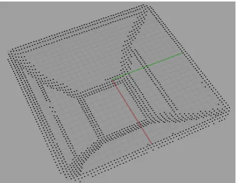
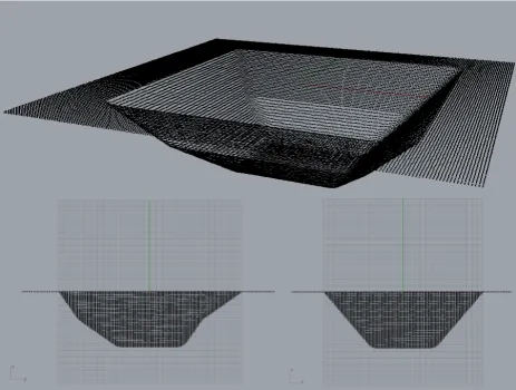
Examples of aGin and a correspondingGout grid (d=1mm) for a flat topped pyramid shape, made out of sheet steel using the AISF process, are presented in Figure 3 and 4 respectively. By inspecting the fig-ures the differences betweenGinandGout can be ob-served, especially with respect to: (i) the degree of concavity on the side walls and (ii) the deformation in the flat area around the edge of the pyramids.
In the case of training set derivation, onceGinand Gout have been derived the next stage is to determine the degree of springback (the error valuee) to be as-sociated with each grid square in Gin. The process
for this is as follows, for each grid square inGin: 1. Find the normal of the centre grid point~n
us-ing vector products. In this manner four nor-mals can be found from the dot products of pairs of 90◦ separated vectors connecting the current grid square centre to its north, south, east and west neighbours.
1The GOM (Gesellschaft f ¨ur Optische Messtechnik mbH)
Figure 2: Springback Calculation.
Figure 3: ExampleGin grid for a flat topped pyramid 3D surface (d=1mm).
Figure 4: ExampleGout grid for a flat topped pyramid 3D surface (d=1mm), corresponding to theGin grid given in Figure 3.
2. Identify the intersection point pint located on Gout by extending each normal~n from Gin to
where they cutsGout.
3. Determine the distance along each normal~n
[image:5.595.39.558.526.628.2]4. The average of the four calculated distances then defines the magnitude of the springback errorei at centre pi, the sign (+or−) defines the direction.
The process is illustrated in Figure 2. Referring to the figure we commence withCin andCout point clo-uds (left hand panel), we the calculate the spring back error for each gird square centre point using vector geometry (middle panel), which is then associated withy each grid square (right hand panel).
ei=
|a(xi−xint) +b(yi−yint) +c(zi−zint)|
p
(a2+b2+c2) (1)
4. Local Geometry Matrix (LGM) Representation
The first 3D surface representation mechanism considered is the Local Geometry Matrix (LGM) me-chanism. The concept of LGMs is founded on the idea of Local Binary Patterns (LBPs) as frequently used with respect to image texture analysis. A local geometry matrix is a n×ngrid describing the loca-tions surrounding an individual point (the point of interest is at the centre of the matrix). Three varia-tion of the LGM representavaria-tion were considered: (i) level one LGMs where the eight closest surround-ing neighbours are considered as shown in Figure 5a (this variation is described in previous work (El-Salhi et al., 2012)), (ii) level two LGMs where the eight surrounding neighbours “one step away” are consid-ered as shown in Figure 5b and (iii) composite LGMs produced by combing level one and two LGMs as shown in Figure 5c. Two different options for gen-erating the values to be stored in the LGM were also considered. The first option was to use the difference in height (δz) between the centre pointpiand each of
itsnneighbouring pointspj(1≤ j≤n). The second was to use the angle, above or below the horizontal, between piand each point pj. Experimentation, de-scribed in (El-Salhi et al., 2012), indicated that com-posite LGMs coupled with δz values proved to be the most effective representation. Whatever the case at the end of the process we have a LGM for each grid point. In the case of the training set this is aug-mented with an error value (calculated as described above). With respect to the LGM representation we
(a) Level one neighbourhood
(b) level two neighbourhood
[image:6.595.314.556.80.175.2](c) Composite neighbourhood
Figure 5: LGM configurations
opted for classifiers that operate using binary valued data, we therefore needed to discretise the data. To this end ranges of possible LGM values was replaced by one of a set of qualitative labels L used to de-scribes the nature of the slope in each of the eight di-rections. An example set of qualitative labels might be{n,l,p}wherenindicates “negative”, l indicates “level” and pindicates “positive”. In the case of the training data required to generate a classifier, ranges of error values were used in a similar manner. Using this labelling, and by ordering the matrix elements (grid points) in a clockwise direction from the top left, a training set record might be described as fol-lows:
hp,p,p,l,n,n,n,l,ei
whereeis the associated springback. In this manner a dataset comprising a collection of LGM “feature vectors” could be constructed to which any one of a number of classifiers could be applied.
5. Local Distance Measure (LDM) Representation
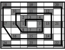
The second 3D surface representation mechanism presented in this paper is the Local Distance Measure (LDM) mechanisms. This is founded on the obser-vation that springback is greater further from edges (Behera et al., 2013). The idea is therefore to de-scribe each grid square in terms of the distance from its centre to the nearest “critical feature point”, where a critical feature point is a grid square that represents an edge of some kind. Thus the LDM process com-mences with the identification of the critical feature points in the input. This was achieved by identifying the eight angular differences α1,α2, ...,α8 between
SE}. If one or more of the angular differenceαiwas
found to be greater than some tolerance measure,ξ, then the centre grid point was considered to be a criti-cal feature point. Once the criticriti-cal feature points had been detected the closest critical point to each grid centre point was determined by adopting a “region growing” process.
The grid sized The tolerance valueξ
2.5 9
5 9
10 15
15 18
[image:7.595.62.265.192.290.2]20 20
Table 1: The most appropriate tolerance value ξ for different grid sizes (d) in the context of critical fea-ture point detection
Equation 2 was used to calculate the minimum distance between the centre grid pointp1= (x1,y1,z1)
and the closest critical point p2= (x2,y2,z2).
d(p1,p2) =
q
(x1−x2)2+ (y
1−y2)2+ (z1−z2)2
(2)
The result is a set of records each describing a grid square location in terms of its critical distance (and, in the case of a training set, its associated springback vale E). Clearly, there are two main factors that af-fect the process of edge detection: (i) the tolerance value ξ and (ii) the grid size d. As the value for ξ increases the number of identified critical feature points will decrease. As the grid size d increases the number of identified critical feature points is also likely to increase because the angular differences be-tween normals is more likely to be large. Conse-quently, in the context of the LDM representation, theξ andd values are related and should be chosen carefully. An additional set of experiments, not re-ported in this paper (but see El-Salhi et al. (2012)), was conducted to identify the most appropriate value of ξ to be associated with each d value. Table 1 presents the main findings of these experiments, these are then the ξ values used with respect to the eval-uation reported later in this paper. The outcomes
when usingd=2.5mm and a number of differentξ values ({15,12,9,5}) to detect critical feature points (edges) in a flat-topped pyramid shape are presented in Figures 6, 7, 8 and 9. From the figures it can be seenξ =9 produces the best performance, when ξ >9 critical feature points remain undiscovered, whenξ <9 the system become too sensitive and too many points are identified.
Whatever the case, as in the case of the LGM rep-resentation, at the end of the process a dataset com-prising a collection of LDM “feature vectors” is ob-tained to which a number of different possible clas-sifiers can be applied.
6. Point Series Representation (PS)
This section presents the PS technique whereby a 3D surface is defined in terms of the local geome-tries surrounding individual grid square neighbour-hoods based on the idea of linearising the key ele-ments of the volume to form a sequence (series) of points. Thus the local,geometry for each grid square will be defined in terms of a point series. The de-sired linearisation can be conducted using a horizon-tal, vertical, “zig-zag” or a spiral linearisation so as to pass through each “key” grid point within an×n neighbourhood centred on the grid square of interest as shown in Figure 10. With respect to the work de-scribed in this paper a spiral linearisation was used as also shown in Figure 10, the numbering indicate the ordering of the linearisation. This linearisation is translated to a curve representation where the x-axis gives the grid square number and the y-axis the δz value associated with this grid square. In this manner we can generate a point series for each centre point pj located in gridGin. In the context of training data each point series was also have associated with it an error label indicating the associated springback value ei.
Figure 6: Critical feature point detection in a flat topped pyramid shape (d=2.5 mm andξ =15).
Figure 7: Critical feature point detection in a flat topped pyramid shape (d=2.5 mm andξ =12).
Figure 8: Critical feature point detection in a flat topped pyramid shape (d=2.5 mm andξ =9).
[image:8.595.38.273.419.600.2] [image:8.595.319.557.426.593.2](DTW) was adopted (Figure 11). DTW operates as follows. Given two point series A={a1,a2,· · ·,an}
and B={b1,b2,· · ·,bm}, a matrix T that has a di-mension of|A| × |B|=n×mis generated, where the value of the (ith,jth) element is obtained according to the Euclidean distance measure (absolute value of distance between two points) d(ith,jth) =|ai−bj|.
After the matrix elements are computed, the simi-larity between two time series (curves) is defined in terms of the length of the “minimum path” across the matrixT from the bottom-left to the top-right corner as shown in Figure 11. Thus the minimum DTW path betweenAandBis defined as follows:
min DTW path(A,B) =min
v u u t
K
∑
k=1wk
(3)
wherewk=d(ith,jth)andmax(n,m)≤K<m+n−
1 (Keogh & Pazzani, 2001; Xi et al., 2006). Note that given two identical curves the shortest path will be along the diagonal and the accumulated distance will be zero.
7. Evaluation
The comparison of the proposed methods was con-ducted using two flat-topped pyramid surfaces (shapes) referred to as the Gonzalo and Modified pyramids (see Figures 12 and 13). From the figures it can be observed that the two surfaces are similar although not identical (one side of the Gonzalo pyramid fea-tures a “bulge”). Some statistical characteristics for theGin grid, with respect to the two shapes, are pre-sented in Table 2. Note that the Modified pyramid features many more points (although both pyramids are similar in size). Each surface was manufactured four times, twice in Steel and twice in Titanium. Hence, we have eightGout grids: (i) Gonzalo steel 1 (GS1),
(ii) Gonzalo Steel 2 (GS2), (iii) Gonzalo titanium 1 (GT1), (iv) Gonzalo titanium 2 (GT2), (v) Modi-fied steel 1 (MS1), (vi) ModiModi-fied Steel 2 (MS2), (vii) Modified titanium 1 (MT1) and (viii) Modified tita-nium 2 (MT2). Some statistics concerning the Gout grids are presented in Table 3.
The evaluation was conducted using a range of grid sizesd={2.5,5,10,15,20}(mm). Consequently
[image:9.595.360.487.125.223.2]Figure 10: Spiral linearisation process for 7×7 patterns.
Figure 11: The minimum path betweenA andB series shown in by the bold diagonal line.
Table 2: Statistical characteristics for the Gin point clouds for the Gonzalo and Modified pyramids:W =
widthmm,L=lengthmm,H=heightmm,A=area of grid (W×L)mm2,N=number of points andD=
density of points permm2(N/A).
Cin W L H A N D
Gonzalo 195 195 43 38025 250847 7.00
[image:9.595.308.535.275.444.2]Figure 12: TheGincloud for Gonzalo steel pyra-mid.
Figure 13: TheGincloud for Modified steel
[image:10.595.38.270.81.256.2]pyra-mid.
Table 3: Statistical characteristics for the Cout point clouds for the Gonzalo and Modified pyramids.
Cout W L H A N D
GS1 194 194 45 37636 421214 11.00
GS2 194 194 44 37636 233480 6.00
GT1 199 189 46 37611 430900 11.00
GT2 195 194 46 37830 185526 5.00
MS1 196 195 45 38220 257436 7.00
MS2 196 195 44 38220 269031 7.00
MT1 195 195 47 38025 394895 10.00
MT2 195 194 46 37830 401186 11.00
the number of generated records (recall that one record represents one grid square) varied for each data set according to the value ofd, as shown in Table 4. For the PS representation a “tolerance” of 0.08 mm, as suggested by BS EN ISO 1101:2005 (BS ISO 1101), was used2. Recall also that a Decision Tree (DT) classifier was adopted with respect to the LGM and LDM techniques (although any other compatible clas-sifier would have been equally appropriate), while k-NN coupled with DTW was used with respect to the PS technique. The results obtained are presented, in terms of both accuracy and Area Under ROC Curve (AUC), in Section 7.1 below.
2BS EN ISO 1101 is a geometrical Product Specification
(GPS) standards. The maximum variation between the techni-cal design and actual (true) geometry is specified according to tolerancevalues included in the specification.
The first two objectives of the experiments were as follows: (i) to identify the most appropriate grid size with respect to each proposed technique and (ii) to identify the most appropriate 3D representation technique for springback prediction. Both these two objectives are discussed, with respect to the results reported in Sections 7.1, 7.2 and 7.3. Additional experiments were conducted to determine w-hether it was possible to generate a generic classifier, one trained on some suitable shape that could be used to predict the springback associated with other shapes. This is discussed further in Section 7.4. Further anal-ysis is presented in Section 7.5, with respect to the second objective, to determine whether the results obtained are indeed statistically significant.
Table 4: Number of records generated for the Gon-zalo and Modified pyramids using different values of d(mm).
d GS1 GS2 GT1 GT2 MS1 MS2 MT1 MT2
2.5 6086 6086 5928 6086 5853 5853 5853 5853
5 1523 1523 1483 1523 1483 1483 1483 1483
10 402 402 381 402 381 381 381 381
15 171 171 171 171 171 171 171 171
20 102 102 102 102 102 102 102 102
7.1. Results
[image:10.595.47.280.366.482.2]a range of grid sizesd={2.5,5,10,15,20}(mm). In the case of the LGM technique a label size of|L|=3 was used as earlier experiments (not reported here) demonstrated that this produced good results. The accuracy and AUC results obtained using the three LGM variations (Level 1 LGM, Level 2 LGM and the Composite LGM) are presented in Tables 5 and 6 respectively, best results are indicated in bold font. With respect to the LDM technique and the consid-ered combinations of the LDM technique with the LGM technique (LDM+Level 1 LGM, LDM+Level 2 LGM and LDM+Composite LGM) Table 7 presents the accuracy results while Table 8 the AUC results (again best results are indicated using a bold font). For the Point Series (PS) technique a range ofn val-ues, describing different n×n neighbourhood con-figurations (n={3,5,7}), were considered. Recall that the PS technique was used in conjunction with k-NN classification and that a tolerance value of 0.08 mm was used when determining the DTW similar-ity between surfaces. Table 9 presents the accuracy results obtained while Table 10 presents the AUC re-sults. The relevance of these results, with respect to the first two evaluation objectives, are presented in the following two sections; Section 7.2 and Section 7.3 respectively.
7.2. Best grid size
This section considers the results presented in the foregoing sections with respect to the identification of the most appropriate grid size, in the context of prediction effectiveness (AUC), with respect to each proposed techniques. The AUC measure was used for this purpose because it takes into account class priors, whilst the accuracy metric does not, AUC is therefore argued to be a better indicator of classifica-tion effectiveness. The three LGM variaclassifica-tions (Level 1 LGM, Level 2 LGM and the Composite LGM) are considered in Section 7.2.1, the LDM technique and combinations of the LDM and LGM techniques (LDM + Level 1 LGM, LDM + Level 2 LGM, LDM + Composite LGM ) are discussed in Section 7.2.2 and the Point Series (PS) technique in Section 7.2.3.
7.2.1. The Best Grid size for LGM Technique
[image:11.595.312.553.272.625.2]Considering the LGM technique and its varia-tions first, from Table 5 it can be observed that high
Table 5: Accuracy results obtained using variations of the LGM representation using a range of values for grid size (d={2.5,5,10,15,20}mm and|L|=3.
Data 3D Proposed Grid size (d) mm
Set Technique 2.5 5 10 15 20
GS1
Level 1 LGM 0.60 0.61 0.62 0.62 0.70 Level 2 LGM 0.60 0.61 0.70 0.65 0.54 Composite LGM 0.60 0.61 0.69 0.69 0.65
GS2
Level 1 LGM 0.83 0.84 0.85 0.88 0.94 Level 2 LGM 0.83 0.84 0.88 0.87 0.84 Composite LGM 0.83 0.84 0.89 0.89 0.93
GT1
Level 1 LGM 0.70 0.70 0.63 0.83 0.78 Level 2 LGM 0.70 0.70 0.65 0.75 0.78 Composite LGM 0.70 0.70 0.66 0.77 0.81
GT2
Level 1 LGM 0.74 0.76 0.73 0.76 0.75 Level 2 LGM 0.74 0.76 0.76 0.79 0.73 Composite LGM 0.74 0.76 0.76 0.85 0.78
MS1
Level 1 LGM 0.65 0.68 0.68 0.83 0.89 Level 2 LGM 0.65 0.68 0.73 0.78 0.75 Composite LGM 0.65 0.68 0.73 0.86 0.86
MS2
Level 1 LGM 0.62 0.67 0.74 0.83 0.93 Level 2 LGM 0.62 0.67 0.78 0.79 0.78 Composite LGM 0.62 0.67 0.78 0.88 0.95
MT1
Level 1 LGM 0.49 0.55 0.62 0.54 0.64 Level 2 LGM 0.49 0.55 0.72 0.61 0.51 Composite LGM 0.49 0.55 0.72 0.68 0.62
MT2
Level 1 LGM 0.54 0.54 0.59 0.64 0.73 Level 2 LGM 0.54 0.54 0.67 0.71 0.69 Composite LGM 0.54 0.54 0.66 0.67 0.71
Average
Table 6: AUC results obtained using variations of the LGM representation using a range of values for ford size (d={2.5,5,10,15,20}mm) and|L|=3.
Data 3D Proposed Grid size (d) mm
Set Technique 2.5 5 10 15 20
GS1
Level 1 LGM 0.66 0.67 0.62 0.73 0.78 Level 2 LGM 0.66 0.67 0.73 0.69 0.71 Composite LGM 0.66 0.67 0.73 0.75 0.76
GS2
Level 1 LGM 0.82 0.83 0.83 0.88 0.94 Level 2 LGM 0.82 0.83 0.96 0.86 0.84 Composite LGM 0.82 0.83 0.96 0.93 0.92
GT1
Level 1 LGM 0.74 0.74 0.69 0.81 0.81 Level 2 LGM 0.74 0.74 0.79 0.79 0.83 Composite LGM 0.74 0.74 0.80 0.83 0.83
GT2
Level 1 LGM 0.76 0.77 0.73 0.82 0.84 Level 2 LGM 0.76 0.77 0.82 0.80 0.80 Composite LGM 0.76 0.77 0.82 0.89 0.87
MS1
Level 1 LGM 0.69 0.70 0.66 0.84 0.86 Level 2 LGM 0.69 0.70 0.78 0.84 0.82 Composite LGM 0.69 0.70 0.78 0.88 0.85
MS2
Level 1 LGM 0.68 0.70 0.76 0.86 0.95 Level 2 LGM 0.68 0.70 0.91 0.87 0.84 Composite LGM 0.68 0.70 0.91 0.88 0.94
MT1
Level 1 LGM 0.50 0.64 0.67 0.71 0.68 Level 2 LGM 0.50 0.64 0.75 0.80 0.64 Composite LGM 0.50 0.64 0.75 0.84 0.72
MT2
Level 1 LGM 0.64 0.63 0.64 0.69 0.76 Level 2 LGM 0.64 0.63 0.74 0.84 0.76 Composite LGM 0.64 0.63 0.73 0.84 0.81
Average
Level 1 LGM 0.69 0.71 0.70 0.79 0.83 Level 2 LGM 0.69 0.71 0.81 0.81 0.78 Composite LGM 0.69 0.71 0.81 0.86 0.84
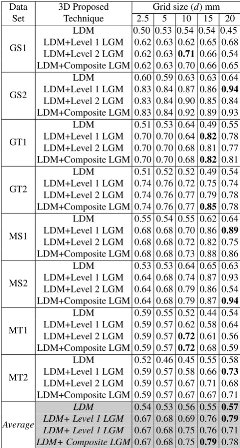
Table 7: Accuracy results obtained using variations of the LDM representation using a range of values for grid size (d={2.5,5,10,15,20}mm).
Data 3D Proposed Grid size (d) mm
Set Technique 2.5 5 10 15 20
GS1
LDM 0.50 0.53 0.54 0.54 0.45
LDM+Level 1 LGM 0.62 0.63 0.62 0.65 0.68 LDM+Level 2 LGM 0.62 0.63 0.71 0.66 0.54 LDM+Composite LGM 0.62 0.63 0.70 0.66 0.65
GS2
LDM 0.60 0.59 0.63 0.63 0.64
LDM+Level 1 LGM 0.83 0.84 0.87 0.86 0.94 LDM+Level 2 LGM 0.83 0.84 0.90 0.85 0.84 LDM+Composite LGM 0.83 0.84 0.92 0.89 0.93
GT1
LDM 0.51 0.53 0.64 0.49 0.55
LDM+Level 1 LGM 0.70 0.70 0.64 0.82 0.78 LDM+Level 2 LGM 0.70 0.70 0.68 0.81 0.77 LDM+Composite LGM 0.70 0.70 0.68 0.82 0.81
GT2
LDM 0.51 0.52 0.52 0.49 0.54
LDM+Level 1 LGM 0.74 0.76 0.72 0.75 0.74 LDM+Level 2 LGM 0.74 0.76 0.77 0.79 0.78 LDM+Composite LGM 0.74 0.76 0.77 0.85 0.78
MS1
LDM 0.55 0.54 0.55 0.62 0.64
LDM+Level 1 LGM 0.68 0.68 0.70 0.86 0.89 LDM+Level 2 LGM 0.68 0.68 0.72 0.82 0.75 LDM+Composite LGM 0.68 0.68 0.73 0.88 0.86
MS2
LDM 0.53 0.53 0.64 0.65 0.63
LDM+Level 1 LGM 0.64 0.68 0.74 0.87 0.93 LDM+Level 2 LGM 0.64 0.68 0.79 0.86 0.54 LDM+Composite LGM 0.64 0.68 0.79 0.87 0.94
MT1
LDM 0.59 0.55 0.52 0.44 0.54
LDM+Level 1 LGM 0.59 0.57 0.62 0.58 0.64 LDM+Level 2 LGM 0.59 0.57 0.72 0.61 0.56 LDM+Composite LGM 0.59 0.57 0.72 0.68 0.59
MT2
LDM 0.52 0.46 0.45 0.55 0.58
LDM+Level 1 LGM 0.59 0.57 0.58 0.66 0.73 LDM+Level 2 LGM 0.59 0.57 0.67 0.71 0.68 LDM+Composite LGM 0.59 0.57 0.67 0.67 0.71
Average
LDM 0.54 0.53 0.56 0.55 0.57
[image:12.595.43.284.271.626.2]Table 8: AUC results obtained using variations of the LDM representation using a range of values for grid size (d={2.5,5,10,15,20}mm).
Data 3D Proposed Grid size (d) mm
Set Technique 2.5 5 10 15 20
GS1
LDM 0.50 0.51 0.50 0.49 0.46
LDM+Level 1 LGM 0.69 0.68 0.65 0.73 0.76 LDM+Level 2 LGM 0.69 0.68 0.75 0.72 0.71 LDM+Composite LGM 0.69 0.68 0.74 0.75 0.75
GS2
LDM 0.50 0.50 0.47 0.47 0.45
LDM+Level 1 LGM 0.82 0.83 0.84 0.90 0.94 LDM+Level 2 LGM 0.82 0.83 0.95 0.86 0.84 LDM+Composite LGM 0.82 0.83 0.96 0.93 0.92
GT1
LDM 0.53 0.54 0.45 0.49 0.61
LDM+Level 1 LGM 0.74 0.74 0.71 0.82 0.80 LDM+Level 2 LGM 0.74 0.74 0.79 0.81 0.84 LDM+Composite LGM 0.74 0.74 0.80 0.85 0.83
GT2
LDM 0.50 0.50 0.45 0.53 0.45
LDM+Level 1 LGM 0.76 0.77 0.72 0.81 0.84 LDM+Level 2 LGM 0.76 0.77 0.81 0.80 0.80 LDM+Composite LGM 0.76 0.77 0.81 0.88 0.87
MS1
LDM 0.57 0.50 0.54 0.47 0.45
LDM+Level 1 LGM 0.71 0.70 0.74 0.85 0.86 LDM+Level 2 LGM 0.71 0.70 0.80 0.87 0.82 LDM+Composite LGM 0.71 0.70 0.80 0.88 0.85
MS2
LDM 0.58 0.50 0.49 0.48 0.45
LDM+Level 1 LGM 0.71 0.71 0.75 0.87 0.96 LDM+Level 2 LGM 0.71 0.71 0.92 0.90 0.84 LDM+Composite LGM 0.71 0.71 0.92 0.87 0.97
MT1
LDM 0.50 0.52 0.50 0.49 0.55
LDM+Level 1 LGM 0.68 0.67 0.67 0.75 0.68 LDM+Level 2 LGM 0.68 0.67 0.75 0.80 0.68 LDM+Composite LGM 0.68 0.67 0.75 0.84 0.71
MT2
LDM 0.59 0.50 0.49 0.58 0.57
LDM+Level 1 LGM 0.68 0.67 0.64 0.73 0.76 LDM+Level 2 LGM 0.68 0.67 0.75 0.86 0.77 LDM+Composite LGM 0.68 0.67 0.75 0.85 0.80
Average
LDM 0.53 0.51 0.49 0.50 0.50
[image:13.595.327.538.277.631.2]LDM+ Level 1 LGM 0.72 0.72 0.72 0.81 0.83 LDM+ Level 2 LGM 0.72 0.72 0.82 0.83 0.79 LDM+ Composite LGM 0.72 0.72 0.82 0.86 0.84
Table 9: The Accuracy results obtained using vari-ations of the the PS representation and a range of values for grid size (d={2.5,5,10,15,20}mm) and neighbourhood size (n={3,5,7}).
Data set n×nPS Grid size (d) mm
2.5 5 10 15 20
GS1
3×3 PS 0.97 0.98 0.98 0.97 0.90
5×5 PS 0.97 0.97 0.98 1.00 0.84 7×7 PS 0.98 0.99 0.94 0.87 0.78
GS2
3×3 PS 0.99 0.98 0.97 0.96 0.96 5×5 PS 0.99 0.97 0.96 0.94 0.92 7×7 PS 0.99 0.98 0.94 0.89 0.67
GT1
3×3 PS 0.99 1.00 0.99 0.94 0.93
5×5 PS 0.99 0.99 0.94 0.94 0.91
7×7 PS 0.98 0.99 0.87 0.79 0.81
GT2
3×3 PS 0.99 0.99 0.99 0.98 0.96
5×5 PS 0.99 0.99 0.96 0.95 0.99 7×7 PS 0.99 0.98 0.88 0.83 0.48
MS1
3×3 PS 0.97 0.97 0.98 0.97 0.97 5×5 PS 0.96 0.96 0.96 0.98 0.91 7×7 PS 0.96 0.97 0.99 0.89 0.75
MS2
3×3 PS 0.96 0.98 0.98 0.97 0.92
5×5 PS 0.96 0.96 0.97 0.97 0.92
7×7 PS 0.97 0.97 0.96 0.92 0.67
MT1
3×3 PS 0.98 0.98 0.98 0.97 0.90
5×5 PS 0.98 0.98 0.96 0.97 0.84
7×7 PS 0.98 0.98 0.92 0.97 0.70
MT2
3×3 PS 0.97 0.96 0.93 0.98 0.82 5×5 PS 0.97 0.96 0.93 0.96 0.99 7×7 PS 0.97 0.96 0.97 0.92 0.56
Avergae
3×3 PS 0.98 0.98 0.98 0.97 0.92
5×5 PS 0.98 0.98 0.96 0.96 0.92
Table 10: The AUC results obtained using variations of the the PS representation and a range of values for grid size (d={2.5,5,10,15,20}mm) and neigh-bourhood size (n={3,5,7}).
Data set n×nPS Grid size (d) mm
2.5 5 10 15 20
GS1
3×3 PS 0.96 0.97 0.96 0.95 0.82 5×5 PS 0.96 0.95 0.97 1.00 0.80 7×7 PS 0.97 0.98 0.92 0.70 0.33
GS2
3×3 PS 0.94 0.89 0.84 0.64 0.78 5×5 PS 0.94 0.89 0.75 0.64 0.73 7×7 PS 0.96 0.93 0.85 0.65 0.50
GT1
3×3 PS 0.97 1.00 0.98 0.76 0.72 5×5 PS 0.96 0.99 0.89 0.70 0.74 7×7 PS 0.93 0.99 0.77 0.57 0.89
GT2
3×3 PS 0.96 0.99 0.97 0.93 0.96 5×5 PS 0.96 0.98 0.85 0.90 0.99 7×7 PS 0.95 0.96 0.72 0.75 0.19
MS1
3×3 PS 0.92 0.92 0.97 0.94 0.87 5×5 PS 0.91 0.92 0.92 0.97 0.62 7×7 PS 0.92 0.95 0.99 0.81 0.67
MS2
3×3 PS 0.94 0.97 0.93 0.92 0.71
5×5 PS 0.94 0.94 0.91 0.93 0.64
7×7 PS 0.95 0.97 0.95 0.86 0.50
MT1
3×3 PS 0.96 0.97 0.94 0.96 0.81
5×5 PS 0.96 0.96 0.89 0.95 0.70
7×7 PS 0.95 0.97 0.72 1.00 0.47
MT2
3×3 PS 0.96 0.94 0.90 0.94 0.73 5×5 PS 0.96 0.94 0.92 0.93 0.98 7×7 PS 0.94 0.93 0.95 0.74 0.25
Avergae
3×3 PS 0.95 0.96 0.94 0.88 0.95
5×5 PS 0.95 0.95 0.89 0.88 0.78
7×7 PS 0.95 0.96 0.86 0.76 0.48
grid sizes tended to produces better accuracy results (best accuracy of 0.95% whend=20), although when d is large the data sets comprise fewer records than when d is small. Similarly, from Table 6 it can be seen that most of the best AUC results were obtained using higher values ofd(best AUC of 0.96 whend=
10). A better understanding of the effect of grid size can be obtained by considering the number of occa-sions that a best AUC result was produced with re-spect to eachd value and each LGM variation. This is presented in Table 11. Note that because we have eightCout clouds (test sets) each row adds up to 8. From this table, it can be seen that the Level 1 LGM technique was able to represent effectively 3D sur-faces using a large grid sizes (d = 20), while the Level 2 LGM technique required smaller grid size (d = 10) to be effective. However, the composite LGM operated best at a compromise d value of 15 mm (recall that the composite LGM technique uses both Level 1 and Level 2 LGMs, a combination of the two).
Table 11: Number of times each grid size (d =
{2.5,5,10,15,20} mm) produced the best perfor-mance, in terms of AUC, with respect to each of the three LGM techniques considered and each of the eight data sets.
Proposed TechniquesGrid size (d) mmBestdvalue 2.5 5 10 15 20
Level 1 LGM 0 0 0 1.5 6.5 20
Level 2 LGM 0 0 4 3 1 10
Composite LGM 0 0 1 5.5 1.5 15
[image:14.595.327.536.491.553.2]best results are obtained using low values of d (al-though the results are not conclusive). When comb-ing the LDM technique with LGM the best d val-ues are comparable with those obtained when using LGMs on their own.
Table 12: Number of times each grid size (d =
{2.5,5,10,15,20} mm) produced the best perfor-mance (in terms of AUC) with respect to each of the four LDM techniques considered and each of the eight data sets.
Proposed Techniques Grid size (d) mmBestdvalue 2.5 5 10 15 20
LDM 3.51.5 0 1 2 2.5
LDM+Level 1 LGM 0 0 0 2 6 20
LDM+Level 2 LGM 0 0 4 3 1 10
LDM+Composite LGM 0 0 1 5 2 15
7.2.3. The Best Grid size for PS Technique
In the case of the Point Series (PS) technique Ta-bles 9 and 10 indicate, although not entirely conclu-sively, that a grid size of d =5 is the most appro-priate. The number of occasions that each grid size produced the best AUC value, with respect to each PS variation and each data set considered, is shown in Table 13. The table confirms that the most appro-priate grid size is d =5. There is little to choose between the PS variations when d is small; it is not until we get to d =20 that some significant differ-ence between the PS variations can be noted. With reference to Table 10 and when d =20 the 3×3 configuration produced the best results (AUC=0.99) while the 7×7 configuration produced the worst re-sults (AUC=0.19). Of course there is a relationship betweennandd, as either is increased a greater area of the surface of interest is “covered”, increasing one and decreasing the other has a neutralising effect. Fi-nally, all three techniques considered operate using different values of d because in each casedis being used in a different manner. With respect to LGMs we wish to setdto a value which optimizes the area cov-ered in terms of the description of the local geometry. With respect to LDMs we wish to setdso as to opti-mize the discovery of edges. With respect to PS we
wish to setd so that the nature of the point series is optimized with respect to classification performance.
Table 13: The occurrences of the best AUC results obtained by 3×3, 5×5 and 7×7 PS for a range of grid sized={2.5,5,10,15,20}.
PS TechniqueGrid size (d) mmBestdvalue 2.5 5 10 15 20
3×3 PS 2 5 1 0 0 5
5×5 PS 2 2 0 2 2 5
[image:15.595.52.275.259.336.2]7×7 PS 1 4 2 1 0 5
Table 14: Some statistics concerning the AUC re-sults obtained from the application of the LGM tech-niques.
LGM Techniques Max Min Median Average SD Level 1 LGM 0.95 0.50 0.74 0.74 0.09 Level 2 LGM 0.96 0.50 0.77 0.76 0.09 Composite LGM 0.96 0.50 0.78 0.78 0.10
Table 15: Some statistics concerning the AUC results obtained from the application of the LDM technique (and its variations).
LDM Techniques Max Min Median Average SD
LDM 0.61 0.45 0.50 0.51 0.04
LDM+Level 1 LGM 0.96 0.64 0.74 0.76 0.08 LDM+Level 2 LGM 0.95 0.67 0.77 0.78 0.07 LDM+Composite LGM 0.97 0.67 0.79 0.79 0.09
7.3. Best Surface Representation Technique
Table 16: Some statistics concerning the AUC results obtained from the application of the PS technique.
PS Techniques Max Min Median Average SD 3×3 PS 1.00 0.64 0.94 0.90 0.09 5×5 PS 1.00 0.62 0.93 0.89 0.10 7×7 PS 1.00 0.19 0.92 0.92 0.22
respect to the LDM technique, from Table 15, it can be noted that the LDM technique on its own did not produce an effective performance compared to its us-age when combined with the LGM technique. The best performance was obtained when LDM was com-bined with the Composite LGM representation (best average AUC value of 0.79). In the case of the PS technique Table 16 demonstrates that this technique produced excellent results, regardless of the size of the neighbourhood the PS technique outperformed the best performing variations of both the LGM and LDM techniques. Overall the most consistent PS technique (that with the smaller standard deviation) was when it was coupled with a 3×3 neighbourhood. Table 17 summarises the best variation for each cat-egory of representation technique (LDM is included in isolation and in combination with the Composite LGM technique).
Table 17: Summary best variation, with respect to AUC, for each representation technique (LDM is in-cluded in isolation and in combination with the Com-posite LGM technique).
Max Min Mode Median Average SD
Composite LGM 0.93 0.75 0.88 0.84 0.86 0.06
LDM 0.59 0.50 0.50 0.57 1.03 1.04
LDM+Composite LGM 0.93 0.75 0.85 0.85 0.86 0.07
3×3 PS 1.00 0.96 0.98 0.98 0.98 0.01
7.4. Generalisation
This section presents the results obtained from training a classifier on one shape and testing it on an-other. The main goal was to determine whether it was possible to generate a generally applicable classifier if it was provided with a suitable shape to train on.
[image:16.595.324.536.432.569.2]The 3×3 neighbourhood PS representation was used for this purpose (withd=5 mm) because earlier ex-periments had indicated that this technique was the most effective (recall that the PS technique was used in conjunction with k-NN classification and that a tolerance value of 0.08 mm was used in the context of DTW similarity). Table 18 presents the results ob-tained in terms of accuracy values, while Table 19 presents the results obtained in terms of AUC val-ues (best results are in bold). From the tables it can be observed again that using the proposed represen-tation a best accuracy and AUC value of 100% and 1.00 could be obtained (when the classifier is trained using GS2). However, the best overall accuracy av-erage was 0.99 while the best overall AUC avav-erage was 0.98. These are excellent results. The results obtained in terms of both AUC and accuracy also in-dicated that, no matter the nature of the 3D surface to be manufactured or the material from which it is to be manufactured, an effective generic classifier can be produced using the proposed PS technique. Table 18: Accuracy results for the generic classifier based on 3×3 PS.
Train
GS1 GS2 GT1 GT2 MS1 MS2 MT1 MT2
Test
GS1 0.960.990.98 0.95 0.89 0.99 0.99 GS2 0.98 1.000.99 0.97 0.91 1.00 0.99 GT1 0.95 0.95 0.970.88 0.89 0.97 0.97 GT2 0.95 0.98 0.98 0.93 0.88 0.99 0.98 MS1 0.980.99 0.99 0.99 0.95 0.98 0.98 MS2 0.96 0.970.99 0.990.98 0.98 0.98 MT1 0.96 0.970.990.98 0.90 0.88 0.98 MT2 0.96 0.980.990.97 0.90 0.87 0.99 Average 0.96 0.970.990.98 0.93 0.90 0.99 0.98
7.5. Statistical Analysis
Table 19: AUC results for the generic classifier based on 3×3 PS.
Train
GS1 GS2 GT1 GT2 MS1 MS2 MT1 MT2
Test
GS1 0.97 0.94 0.93 0.96 0.91 0.96 0.98 GS2 0.99 0.99 0.921.00 0.96 1.00 0.99 GT1 0.84 0.87 0.95 0.64 0.66 0.94 0.94 GT2 0.81 0.91 0.98 0.65 0.61 0.99 0.95 MS1 0.980.99 0.990.98 0.95 0.98 0.97 MS2 0.95 0.96 0.991.00 0.98 0.97 0.97 MT1 0.85 0.880.960.94 0.62 0.59 0.95 MT2 0.901.000.98 0.93 0.65 0.63 0.99 Average 0.90 0.940.980.95 0.79 0.76 0.98 0.96
of the techniques to determine whether the results produced were truly significant or not with respect to the AUC measure. On completion of the Fried-man test, the Nemenyi test was used to identify the Critical Distance (CD) between the techniques where the techniques are significantly different from each other. Broadly, CD is normally used to examine where the significant differences are actually occured be-tweenindividualtechniques. This kind of statistical analysis is increasingly being used in the field of data mining and more specifically in the context of clas-sification (Han, 2005; Tan et al., 2005). A number of different approaches have been proposed to con-duct such comparisons. With respect to classification techniques the following are of note: (i) the paired t-test, (ii) the Wilcoxon Signed-Rank Test, (iii) the ANOVA test and (iv) the Friedman test3. The Fried-man test offers two advantages over the other tech-niques: (i) ease of computation and interpretation and (ii) its ability to demonstrate the classification performance in terms of a ranking rather than vague averages (Garc´ıa et al., 2009b)). The Friedman test was thus chosen to evaluate the performance of the different proposed techniques with respect to this pa-per. In addition to the practical advantages offered by the Friedman test, it was also chosen because:
• There is no guarantee that the data (AUC re-sults obtained from the proposed techniques) follow the normal (Gaussian) distribution.
3For more detail on these tests (Garc´ıa et al., 2009a,b;
Tsumoto, 2009).
• It is recommended (Demˇsar, 2006) for use with “matched” (related) data sets while the ANOVA test is recommended for use with “unrelated” data sets.
With respect to the work described in this paper, the Gonzalo and Modified data sets were considered to be related data sets given that both describe flat-topped pyramids. Therefore, the Friedman test was consid-ered to be the most suitable statistical test. Therefore, The followingNull hypothesis(H0) and the
Alterna-tive hypothesis(H1) were established.
H 0. There is no significant difference between the proposed classifiers.
H 1. There is a significant difference between the proposed classifiers.
The Friedman statistical test is commenced by rankingthe classification techniques with respect to each data set separately. Then, the average rank for each classification techniques is obtained from across the data sets. The Friedman test statistic is then cal-culated as follows (Demˇsar, 2006; Friedman, 1940; Fisher & Yates, 1970):
χF2 = 12n k(k+1)
"
k
∑
i=1µi2−k(k+1)
2
4 #
(4)
where: (i) n is the number of data sets, (ii) k is the number of classification techniques and (iii)µiis the
average rank for classification technique i which in turn is calculated as follows:
µi=
1 n
n
∑
j=1Rj (5)
hypothesis can be rejected and the Nemenyi test (Ne-menyi, 1963) applied. The Nemenyi test operates us-ing the “distance” between the average rankus-ings of the individual techniques. If this distance is greater than a Critical Difference (CD), calculated using Equa-tion 6, then the performance is considered to be dis-tinct. To qualify the strength of evidences against the null hypothesis, ap-valueis calculated. Thep-value is defined as the probability of obtaining a result that is at least as extreme as the one we actually obtained assuming that the null hypothesis is true. Therefore, if the p-value is not smaller than α, the test is in-conclusive and more evidences will be required to support the alternative hypothesis (H1).
CD=qα,∞,k r
k(k+1)
12n (6)
Where the critical value for qα,∞,k is based on the Studentized range statistic (Demˇsar, 2006). The per-formance of individual techniques is considered to be distinct if the difference between their average rank-ings differs by at least the CD.
The Friedman test was applied with respect to the proposed techniques in the context of the evaluation data sets. Two different cases were considered: (i) where the classification techniques was trained and tested on the same data set and (ii) where the clas-sification techniques was trained on one data set and tested on another. Each is considered in further detail in the following two sections.
7.5.1. Testing and training on the same dataset The Friedman statistical test was first applied to our four different technique with respect to then=8 Gonzalo and Modified data sets (GS1, GS2, GT1, GT2, MS1, MS2, MT1 and MT2). Table 20 presents the rankings (indicated in parentheses) and the aver-age ranks µ for thek =4 proposed techniques (ac-cording to the best AUC values). From the table, it can be seen that the best average rank, 1.25, was achieved by the PS technique. The Friedman statis-tic, calculated using Equation 4 with k−1=3 de-grees of freedom, is then:
χF2 = 12×8 4×(5)
28.91−4×(5) 2
4
=4.80×3.91
=18.77
The χ2 threshold value withα =0.05 and 3 de-gree of freedom (null distribution) is 14.07. Given that: (i) the calculated Friedman test value of χF2 = 18.77 is greater than the critical value 14.07, and (ii) p-value = 0.009 which is less than the α value of 0.05 (Abramowitz & I.A. Stegun, 1964; Johnson et al., 1995); the Null Hypothesis (H0), which states
that there is no significant differences in the average ranks, can be rejected to confirm that the operation of thek=4 proposed classifiers generated on the same data sets are significantly different from each other. According to the Nemenyi test the operation of the individual classifiers is also significantly different if the difference between their average ranks is more than or equalCD=1.17, calculated as follows:
CD=2.57×
r 4(5)
12×8
=2.57×0.46
[image:18.595.351.511.96.165.2]=1.17
Figure 14 shows the ranked performance for the k=4 proposed techniques along with Nemenyis crit-ical difference (CD) measure to highlight the tech-niques which are significantly different to each other. In the figure, the head is the average rank while the tail indicates the CD value. From the figure, it can be seen that the PS technique was ranked first and that its operation is significantly different with respect to both the LDM and the composite LGM techniques because as they are overlapped. However, there is no significant difference between the operation of PS and LDM + composite LGM as the difference be-tween their average ranks is 0.88 < 1.17 (the CD value).
Table 20: The best AUC results for the proposed techniques (variations) with respect to each 3D representation technique using the same data set to train and test the classifier.
GS1 GS2 GT1 GT2 MS1 MS2 MT1 MT2 µi
Composite LGM 0.73 (3)0.96 (1.5)0.80 (2.5) 0.82 (2) 0.78 (3) 0.91 (3) 0.75 (2.5) 0.73 (3) 2.56 LDM 0.50 (4) 0.50 (4) 0.53 (4) 0.50 (4) 0.57 (4) 0.58 (4) 0.50 (4) 0.59(4) 4.00 LDM+ Composite LGM 0.74 (2)0.96 (1.5)0.80 (2.5) 0.81 (3) 0.80 (2) 0.92 (2) 0.75 (2.5) 0.75 (2) 2.19 Point Series 0.96 (1)0.95 (3) 0.90 (1) 0.95 (1) 0.97 (1) 0.95 (1) 0.92 (1) 0.91 (1) 1.25
∑kj=1µ2j = 28.91
[image:19.595.308.556.231.285.2]Friedman test statistic = 18.77 (p-value=0.009)
Figure 14: The average rank (µi) associated with CD
value for the classifiers generated using same data sets.
presents the average AUC values obtained in each case. The calculated Friedman statistic with its asso-ciated p-value(as shown in the table) strongly con-firmed again that the PS technique produces the best performance according to its average ranking. Again we can also observe that there is a significant statisti-cal difference between the operation of PS and both the LDM and Composite LGM techniques. In sum-mary, when considering the AUC performance mea-sures, it can be concluded that PS technique yields the best performance while the LDM technique per-forms significantly worse than the other proposed tech-niques. However, the operation of two individual classification techniques (in some cases) yielded clas-sification performances whose differences are not sta-tistically significant such as in the case of (i) Com-posite LGM and the combined LDM + ComCom-posite LGM, (ii) PS and the combined LDM + Composite LGM and (iii) LDM and Composite LGM as shown in Figure 15.
8. Conclusion
This paper has presented three different techniques (LGM, LDM and PS) to represent 3D surfaces for the purpose of building classifiers to predict a phe-nomena known as “springback”. The novelty of the proposed techniques is their ability to capture the
na-Figure 15: The average rank (µi) associated with CD
value for the classifiers generated using different data sets.
ture of the local geometries associated with the 3D surfaces of interest. A Springback Prediction Frame-work was also proposed to generate springback pre-dictors (classifiers) and to apply them. The LGM technique represented the points on a 3D surface us-ing a concept similar to local binary patterns. The LDM technique represented the points in terms of their proximity to the nearest critical feature (edges). The PS technique represented the surface in terms of spiral linearisation curves. Two flat-topped pyramid shapes (Gonzalo and Modified) were used for evalu-ation purposes.
The main findings were as follows:
• The proposed techniques could be effectively used to represent 3D surfaces in a format suited to classifier generation.
• The PS technique outperforms the other tech-niques in terms of both AUC and accuracy, some excellent results were obtained.
Table 21: The best AUC results for the proposed techniques (variations) with respect to each 3D representation technique using different data set to train and test the classifier.
GS1 GS2 GT1 GT2 MS1 MS2 MT1 MT2 µi
Composite LGM 0.70 (3) 0.74 (3) 0.75 (3) 0.81 (3) 0.82 (3) 0.80 (3) 0.76 (3) 0.76 (3) 3.00 LDM 0.52 (4) 0.50 (4) 0.61 (4) 0.50 (4) 0.60 (4) 0.60 (4) 0.50 (4) 0.60(4) 4.00 LDM+ Composite LGM 0.94 (2) 0.90 (2) 0.89 (2) 0.97 (2) 0.92 (2) 0.95 (1.5) 0.93 (2) 0.86 (2) 1.94 Point Series 0.99 (1) 1.00 (1) 0.99 (1) 1.00 (1) 1.00 (1)0.95 (1.5)1.00 (1) 0.99 (1) 1.06
∑kj=1µ2j = 29.88
Friedman test statistic = 23.42 (p-value=0.001)
• Similarly the application of the Friedman test demonstrated that there isno significant differ-ence between the PS and the combined LDM + composite LGM technique (using either the same/different data set), although the PS tech-nique produced some very good results.
Overall these were very encouraging results indicat-ing that the proposed techniques, especially the PS technique, could be effectively used for springback prediction and consequent mitigation with respect to sheet metal forming processes such as AISF. For fu-ture work the research team intend to investigate mech-anisms to propose corrections to the input cloud for a given shape so as to produced a corrected input cloud Ccorr in order to compensate for the springback in-troduced during manufacturing in the context of pro-cesses such as AISF process. This will also require a suitable format for theCcorr cloud to facilitate manu-facturing. The authors are also interested in produc-ing an “intelligent process model” where the Ccorr cloud is iteratively refined until the predicted shape (generated from Ccorr using classification processes of the form described in this paper) is equivalent to Cin (the desired shape).
9. Acknowledgement
The research leading to the results presented in this paper has received funding from the European Union Seventh Framework Programme (FP7/2007-2013) under grant agreement number 266208 and par-tially by Hashemite University in Zarqa, Jordan.
References
Abramowitz, M., & I.A. Stegun, I. (1964). Handbook of Math-ematical Functions: With Formulars, Graphs, and
Mathe-matical Tables. Applied mathematics series. New York : Dover Publications.
Adams, D. (2013). A highly-effective Incremental/Decremental Delaunay Mesh-Generation Strategy for Image Representa-tion. Signal Process.,93, 749–764.
Alexa, M., Behr, J., Cohen, D., Fleishman, S., Levin, D., & Silva, C. (2001). Point Set Surfaces. InProceedings of the conference on Visualization ’01VIS ’01 (pp. 21–28). Wash-ington, DC, USA: IEEE Computer Society.
Ayache, N. (1995). Medical computer vision, virtual reality and robotics. Image and Vision Computing,13, 295 – 313. Behera, A. K., Verbert, J., Lauwers, B., & Duflou, J. (2013).
Tool Path Compensation Strategies for Single Point Incre-mental Sheet Forming using Multivariate Adaptive Regres-sion Splines. Computer-Aided Design,45, 575 – 590. Berger, H., Klein, M., & Mller, T. (2011). Deformation and
vi-bration measurement and data evaluation on large structures employing optical measurement techniques. In T. Proulx (Ed.), Rotating Machinery, Structural Health Monitoring, Shock and Vibration, Volume 5Conference Proceedings of the Society for Experimental Mechanics Series (pp. 547– 554). Springer New York.
Biasotti, S., Giorgi, D., Spagnuolo, M., & Falcidieno, B. (2008). Reeb Graphs for Shape Analysis and Applications. Theoretical Computer Science,392, 5 – 22.
Breiman, L., Friedman, J., Stone, C., & Olshen, R. (1984). Classification and Regression Trees. (1st ed.). Chapman and Hall/CRC.
BS ISO 1101 (2005). BS ISO 1101:2005 Geometrical Product Specifications (GPS) - Geometrical tolerancing - Tolerances of form, orientation, location and run-out- Generalities, def-initions, symbols, indications on drawings.
Cafuta, G., Mole, N., & Łtok, B. (2012). An enhanced displace-ment adjustdisplace-ment method: Springback and thinning compen-sation. Materials and Design,40, 476 – 487.
Chatti, S. (2010). Effect of the Elasticity Formulation in Finite Strain on Springback Prediction.Computers and Structures, 88, 796 – 805.
Chatti, S., & Hermi, N. (2011). The Effect of Non-linear Re-covery on Springback Prediction.Computers and Structures, 89, 1367 – 1377.
Demoly, F., Toussaint, L., Eynard, B., Kiritsis, D., & Gomes, S. (2011). Geometric Skeleton Computation Enabling Concur-rent Product Engineering and Assembly Sequence Planning. Computer-Aided Design,43, 1654 – 1673.
Demˇsar, J. (2006). Statistical comparisons of classifiers over multiple data sets. J. Mach. Learn. Res.,7, 1–30.
El-Salhi, S., Coenen, F., Dixon, C., & Khan, M. (2012). Identi-fication of correlations between 3d surfaces using data min-ing techniques: Predictmin-ing sprmin-ingback in sheet metal form-ing. In M. Bramer, & M. Petridis (Eds.), Research and Development in Intelligent Systems XXIX (pp. 391–404). Springer London.
Farin, G., Hoschek, J., & Kim, M. (2002). Handbook of Com-puter Aided Geometric Design [electronic resource]. Else-vier Science & Technology.
Firat, M., Kaftanoglu, B., & Eser, O. (2008). Sheet Metal Form-ing Analyses With An Emphasis On the SprForm-ingback Defor-mation. Journal of Materials Processing Technology,196, 135 – 148.
Fisher, R., & Yates, F. (1970). Statistical Tables for Biologi-cal,Agricultural,and Medical Research: 6th Ed Rev and Enl. Hafoor.
Fresno, M., Vnere, M., & Clausse, A. (2009). A combined re-gion growing and deformable model method for extraction of closed surfaces in 3d{CT}and{MRI}scans. Computer-ized Medical Imaging and Graphics,33, 369 – 376. Friedman, M. (1940). A Comparison of Alternative Tests of
Significance for the Problem of m Rankings. The Annals of Mathematical Statistics,11, 86–92.
Fu, Z., Mo, J., Chen, L., & Chen, W. (2010). Using Ge-netic Algorithm-Back Propagation Neural Network Predic-tion and Finite-Element Model SimulaPredic-tion to Optimize the Process of Multiple-Step Incremental Air-Bending Forming of Sheet Metal.Materials and Design,31, 267 – 277. Garc´ıa, S., Fern´andez, A., Luengo, J., & Herrera, F. (2009a).
A study of statistical techniques and performance measures for genetics-based machine learning: Accuracy and inter-pretability. Soft Comput.,13, 959–977.
Garc´ıa, S., Molina, D., Lozano, M., & Herrera, F. (2009b). A study on the use of non-parametric tests for analysing the evolutionary algorithms’ behaviour: A case study on the cec’2005 special session on real parameter optimisation. Journal of Heuristics,15, 617–644.
Ghanei, A., Soltanian-Zadeh, H., & Windham, J. (1998). A 3d deformable surface model for segmentation of objects from volumetric data in medical images. Computers in Biology and Medicine,28, 239 – 253.
Goldfeather, J., Hultquist, J. P., & Fuchs, H. (1986). Fast Constructive-Solid Geometry Display in the Pixel-Powers Graphics System. SIGGRAPH Comput. Graph., 20, 107– 116.
Guo, Z., Zhang, L., & Zhang, D. (2010). A Completed Mod-eling of Local Binary Pattern Operator for Texture Classifi-cation. IEEE Transactions on Image Processing,19, 1657– 1663.
GW, B. (1983). Errors, types i and ii. American Journal of
Diseases of Children,137, 586–591.
Han, J. (2005). Data Mining: Concepts and Techniques. San Francisco, CA, USA: Morgan Kaufmann Publishers Inc. Hao, W., & Duncan, S. (2011). Optimization of Tool Trajectory
for Incremental Sheet Forming Using Closed Loop Control. InAutomation Science and Engineering (CASE), 2011 IEEE Conference on(pp. 779 –784).
Hoppe, H., DeRose, T., Duchamp, T., McDonald, J., & Stuet-zle, W. (1992). Surface reconstruction from unorganized points. SIGGRAPH Comput. Graph.,26, 71–78.
Hsiao, S., & Chen, R. (2013). A study of surface reconstruction for 3d mannequins based on feature curves.Computer-Aided Design, .
Hubeli, A., & Gross, M. (2000).A survey of Surface Represen-tations for Geometric Modeling. Technical Report.
Izquierdo, E., & Ohm, J. (2000). Image-based rendering and 3d modeling: A complete framework. Signal Processing: Image Communication,15, 817 – 858.
Jahanshahi, M., & Masri, S. (2012). Adaptive vision-based crack detection using 3d scene reconstruction for condition assessment of structures. Automation in Construction, 22, 567 – 576.
Jain, R., Kasturi, R., & B.G.Schunck (1995). Machine Vision. McGraw-Hill series in computer science. McGraw-Hill. Jeswiet, J., Micari, F., Hirt, G., Bramley, A., Duflou, J., &
Allwood, J. (2005). Asymmetric Single Point Incremen-tal Forming of Sheet MeIncremen-tal. CIRP Annals - Manufacturing Technology,54, 88 – 114.
Johnson, N., Kotz, S., & Balakrishnan, N. (1995). Continu-ous univariate distributions. Number v. 2 in Wiley series in probability and mathematical statistics: Applied probability and statistics. Wiley & Sons.
Keogh, E. J., & Pazzani, M. J. (2001). Derivative Dynamic Time Warping. In In SIAM International Conference on Data Mining.
Khan, M., Coenen, F., Dixon, C., & El-Salhi, S. (2012). Finding Correlations Between 3-d Surfaces: A study in Asymmetric Incremental Sheet Forming. InProc. Machine Learning and Data Mining in Pattern Recognition (MLDM’12), Springer LNAI 7376(pp. 336–379).
Liu, W., Liang, Z., Huang, T., Chen, Y., & Lian, J. (2008). Process Optimal Ccontrol of Sheet Metal Forming Spring-back Based on Evolutionary Strategy. InIntelligent Control and Automation, 2008. WCICA 2008. 7th World Congress on(pp. 7940 –7945).
Liu, W., Liu, Q., Ruan, F., Liang, Z., & Qiu, H. (2007). Spring-back Prediction for Sheet Metal Forming Based on GA-ANN Technology. Journal of Materials Processing Tech-nology,187-188, 227 – 231.
Lu, G., & Sajjanhar, A. (1999). Region-based Shape Repre-sentation and Similarity Measure Suitable for Content-based Image Retrieval. Multimedia Syst.,7, 165–174.
Switzerland: Eurographics Association.
Narasimhan, N., & Lovell, M. (1999). Predicting Springback in Sheet Metal Forming: An Explicit to Implicit Sequential Solution Procedure.Finite Elements in Analysis and Design, 33, 29 – 42.
Nasrollahi, V., & Arezoo, B. (2012). Prediction of Spring-back in Sheet Metal Components With Holes on the Bending Area, Using Experiments, Finite Element and Neural Net-works.Materials and Design,36, 331 – 336.
Nemenyi, P. (1963). Distribution-free multiple comparisons. Ph.D. thesis New Jersey, USA.
Pinto, T., Kohler, C., & Albertazzi, A. (2012). Regular Mesh Measurement of Large Free Form Surfaces Using Stereo Vi-sion and Fringe Projection. Optics and Lasers in Engineer-ing,50, 910 – 916.
Quinlan, J. (1986). Induction of Decision Trees. Machine Learning,1, 81–106.
Quinlan, R. (1993). C4.5: Programs for Machine Learning. San Mateo, CA: Morgan Kaufmann Publishers.
Roth, G., & Wibowoo, E. (1997). An Efficient Volumetric Method for Building Closed Triangular Meshes from 3D Im-age and Point Data. InIn Graphics Interface 97(pp. 173– 180).
Sakoe, H., & Chiba, S. (1990). Readings in speech recognition. chapter Dynamic Programming Algorithm Optimization for Spoken Word Recognition. (pp. 159–165). San Francisco, CA, USA: Morgan Kaufmann Publishers Inc.
Song, I., & Yang, J. (2011). A scene Graph Based Visualiza-tion Method for Representing Continuous SimulaVisualiza-tion Data. Computers in Industry,62, 301 – 310.
Soucy, M., & Laurendeau, D. (1995). A general surface ap-proach to the integration of a set of range views. Pattern Analysis and Machine Intelligence, IEEE Transactions on, 17, 344–358.
Strano, M. (2005). Technological representation of forming limits for negative incremental forming of thin aluminum sheets. Journal of Manufacturing Processes,7, 122 – 129. Tan, P., Steinbach, M., & Kumar, V. (2005). Introduction to
Data Mining, (First Edition). Boston, MA, USA: Addison-Wesley Longman Publishing Co., Inc.
Tisza, M. (2004). Numerical Modelling and Simulation in Sheet Metal Forming.Journal of Materials Processing Tech-nology,151, 58 – 62.
Tsumoto, S. (2009). Contingency matrix theory: Statistical de-pendence in a contingency table.Information Sciences,179, 1615 – 1627.
Wei, L., & Keogh, E. (2006). Semi-supervised time series clas-sification. InProceedings of the 12th ACM SIGKDD interna-tional conference on Knowledge discovery and data mining KDD ’06 (pp. 748–753). New York, NY, USA: ACM. Wettschereck, D. (1994). A study of Distance-based Machine
Learning Algorithms. Ph.D. thesis Corvallis, OR, USA. Wu, X., Kumar, V., Quinlan, J. R., Ghosh, J., Yang, Q.,
Mo-todai, H., McLachlan, G., Ng, A., Liu, B., Yu, P., Zhou, Z., Steinbach, M., Hand, D., & Steinberg, D. (2007). Top 10 Algorithms in Data Mining.Knowl. Inf. Syst.,14, 1–37.
Xi, X., Keogh, E., Shelton, C., Wei, L., & Ratanamahatana, C. (2006). Fast time series classification using numerosity reduction. InProceedings of the 23rd international confer-ence on Machine learningICML ’06 (pp. 1033–1040). New York, NY, USA: ACM.