rsif.royalsocietypublishing.org
Research
Cite this article:
Davis S, Abbasi B, Shah S,
Telfer S, Begon M. 2015 Spatial analyses of
wildlife contact networks.
J. R. Soc. Interface
12
: 20141004.
http://dx.doi.org/10.1098/rsif.2014.1004
Received: 7 September 2014
Accepted: 27 October 2014
Subject Areas:
environmental science, biomathematics
Keywords:
epidemiology, mathematical model, field vole,
Microtus agrestis
, graph, dissimilarity measure
Author for correspondence:
Stephen Davis
e-mail: stephen.davis@rmit.edu.au
Electronic supplementary material is available
at http://dx.doi.org/10.1098/rsif.2014.1004 or
via http://rsif.royalsocietypublishing.org.
Spatial analyses of wildlife contact
networks
Stephen Davis
1, Babak Abbasi
1, Shrupa Shah
1, Sandra Telfer
2and Mike Begon
31School of Mathematical and Geospatial Sciences, RMIT University, Melbourne, Victoria 3001, Australia 2School of Biological Sciences, University of Aberdeen, Zoology Building, Tillydrone Avenue,
Aberdeen AB24 2TZ, UK
3Department of Evolution, Ecology and Behaviour, University of Liverpool, Crown Street, Liverpool L69 7ZB, UK
Datasets from which wildlife contact networks of epidemiological importance can be inferred are becoming increasingly common. A largely unexplored facet of these data is finding evidence of spatial constraints on who has contact with whom, despite theoretical epidemiologists having long realized spatial constraints can play a critical role in infectious disease dynamics. A graph dissimilarity measure is proposed to quantify how close an observed contact network is to being purely spatial whereby its edges are completely deter-mined by the spatial arrangement of its nodes. Statistical techniques are also used to fit a series of mechanistic models for contact rates between individuals to the binary edge data representing presence or absence of observed contact. These are the basis for a second measure that quantifies the extent to which contacts are being mediated by distance. We apply these methods to a set of 128 contact networks of field voles (Microtus agrestis) inferred from mark– recapture data collected over 7 years and from four sites. Large fluctuations in vole abundance allow us to demonstrate that the networks become increas-ingly similar to spatial proximity graphs as vole density increases. The average number of contacts,kkl, was (i) positively correlated with vole density across the range of observed densities and (ii) for two of the four sites a saturating function of density. The implications for pathogen persistence in wildlife may be that persistence is relatively unaffected by fluctuations in host density because at low density kkl is low but hosts move more freely, and at high densitykklis high but transmission is hampered by local build-up of infected or recovered animals.
1. Introduction
There is growing interest among disease ecologists in elaborating contact net-works in wildlife populations and the likely consequences for the spread of pathogens or parasites [1–8]. Theoretical studies have, in particular, shown that (i) pathogens tend to spread rapidly and easily on networks containing small numbers of highly connected individuals and (ii) if those highly connected indi-viduals can be targeted for either vaccination or removal then it becomes easier to prevent an outbreak or mitigate its effects [9]. Hence, a focus of recent studies has often been the detection of high individual heterogeneity in numbers of contacts, and whether characteristics such as age, sex or size might be used to predict which individuals have the highest numbers of contacts. By contrast, analyses that quan-tify spatial constraints on who has contact with whom have largely been absent, even though spatial constraints are capable of critically affecting infectious disease dynamics [10,11]. Craftet al.’s [3] study of contacts between prides of Serengeti lions is an exception, but the approach is highly tailored to the unique datasets arising from the Serengeti Lion Project. Here we propose two approaches: (i) graph dissimilarity measures that quantify how close an observed network is to being a proximity graph (i.e. one in which the edges of a network are
purely determined by the spatial arrangement of the nodes) and (ii) maximum-likelihood approaches to quantify spatial constraints and judge between competing network models. Finally, we fit a class of good-get-richer network models [12,13] that incorporate and quantify both spatial constraints and individual heterogeneity. We apply all of these approaches to a set of 128 contact networks constructed from a large mark– recapture dataset on field voles (Microtus agrestis) collected over a 7-year period.
The role of spatial constraints in determining the dynamics of infectious disease is particularly pertinent for territorial animal populations, where the question arises as to whether territoriality offers a level of protection from disease outbreaks. In territorial populations, two animals may normally have con-tact only if their home ranges overlap, with exceptions arising from rare long distance dispersal events or nomadic individ-uals. Infectious diseases of such populations must overcome what is effectively a spatial barrier if they are to spread and persist; transmission must occur frequently enough to escape local build-up of infected and recovered animals and avoid fade-out. Such spatial effects can be understood to slow an epidemic down in the same way as clustered contact patterns, or the presence of short loops in networks [14]. The effect is that infectious individuals are more likely to have neighbours that are in the recovered state, and also neighbours that are infected, which they may then ‘compete’ with for the few remaining sus-ceptibles. In such circumstances, the use of epidemiological theory based on random mixing of hosts overestimates the abil-ity of the pathogen to spread, undermining, for example, the use of the basic reproduction number,R0, to predict threshold
conditions for outbreaks. This has been well illustrated for the occurrence of epizootics of sylvatic plague (Yersinia pestis infection) in populations of great gerbils (Rhombomys opimus) in Central Asia [15,16].
More generally, the concern of epidemiologists with con-tact networks can be interpreted as an acknowledgement that the transmission of infection occurs at the individual level but its epidemiological consequences are played out at the popu-lation level, and that it is important to understand how the two are related [17]. In particular, it would be valuable to understand whether certain contact structures translate into the canonical density- and frequency-dependent transmission functions or into variants of these and intermediates between them that have been proposed (e.g. [18,19]). Here, therefore, we also explore these connections, as data from the same field vole system have previously been analysed to identify and interpret the transmission function for cowpox virus transmission that best fits population-level data [18].
2. Material and methods
2.1. Trapping data and field sites
The study took place in Kielder Forest, a man-made spruce forest occupying 620 km2, situated on the English–Scottish border (558130N, 28330W). Field voles inhabit grassy clear-cuts that
rep-resent 16–17% of the total area, but are completely absent from forested areas that isolate the clear-cuts. Clear-cuts range in size from 5 to 100 ha. Field vole populations at Kielder fluctuate cyclically with a 3–4 year period [20]. Voles were trapped in four similar-sized clear-cuts, in two areas of the forest approximately 12 km apart, between May 2001 and March 2007. In the Kielder catchment, Kielder Central Site (KCS) and Plashett’s Jetty (PLJ) are situated
4 km apart. In the Redesdale catchment, Black Blake Hope (BHP) and Rob’s Wood (ROB) are 3.5 km apart. Thus, these four popu-lations were far enough apart, with sufficient forest between them, to be considered as effectively independent replicates.
Populations were trapped in ‘primary’ sessions every 28 days from March to November, and every 56 days from November to March. Each site had a permanent 0.3 ha live-trapping grid con-sisting of 100 Ugglan Special Mousetraps (Grahnab, Marieholm, Sweden), in optimal habitat dominated byDeschampsia cespitosa,
Agrostis tenuisandJuncus effusus. Traps were set at 5 m intervals and baited with wheat and carrots. Traps were pre-baited with a slice of carrot and a few grams of oats 3 days before each trap-ping session, set at approximately 18.00 on the first day and checked five times (referred to ‘secondary’ sessions; a ‘primary session’ thus refers to a cluster of five ‘secondary’ sessions) at roughly 12 h intervals starting and ending at dawn and dusk, respectively. Individual animals were identified using subcu-taneous microchip transponders (AVID plc, East Sussex, UK) injected under the skin at the back of the neck. Mass, sex and reproductive status (assigned according to the external appear-ance of reproductive organs) were recorded at the time of first capture in each primary session. Estimates of total population size were derived in program MARK using Huggin’s closed capture model within a robust design [21].
We formed networks from the mark–recapture data by sup-posing each vole trapped was a node of a spatial network. A spatial location for each node was determined as the average position of the traps it was caught in, with trap location weighted by the number of times the vole was caught in that trap. This follows the practice of other wildlife epidemiologists working with similar data [1–8]. An edge was inserted into the network whenever two voles were caught in at least one common trap over the primary trapping sessions being considered. Thus, multiple edges are avoided and the degree of a node (the number of edges connected to it) can be interpreted as the number of unique contacts a vole has over the period of obser-vation. There is potentially an important difference between the rate of contact that includes repeated contacts between the same individuals and the rate at which new contacts are made, and we note that it is also possible to form networks that do include repeated contacts and hence multiple edges. We note that there are a number of other constructions possible from these data that would form slightly different sets of networks. One could be more ‘strict’ about what constitutes indirect contact by having weighted edges (number of traps in common) and then thresholding on the weights to produce simple networks. There are also many ways to define the spatial location of the node set, using either a subset of the trap locations or a different measure of central tendency.
Exploratory work indicated that the contact networks based on a single primary trapping session have no, or very few, edges when the vole densities are low. So that we could consider how the net-works varied with population density we considered combining trapping sessions to form the networks. Voles are sometimes seen in only one trapping session and then never again, but for much of the time a vole is seen in two or more consecutive trapping sessions. Two trapping sessions hence provided a better basis to define a geographical location for each vole (more trap locations) and defined more edges so that even at the lowest vole densities the networks had a reasonable number of edges. When three (or more) trapping sessions are combined (see the electronic sup-plementary material for a comparison) an edge can represent anything from a vole visiting a trap two months after another did, or a vole visiting a trap the next night. We therefore chose to form networks from pairs of consecutive trapping sessions. At each site, there were 64 trapping sessions, and hence 32 networks were formed for each of the four sites, with each network derived from a consecutive pair of primary trapping sessions and each
rsif.r
oy
alsocietypublishing.org
J.
R.
Soc.
Interfa
ce
12
:
20141004
trapping session appearing in only one network. This set of 128 networks represents a range of contact patterns, occurring at different times of the year and at different vole densities.
2.2. Basic graph measures
For each of the 128 contact networks, we calculated the mean degree, kkl to estimate the average rate of contact, and the coefficient of variation (CV) of the degree distribution. We tested whether there was more support from the data for a linear, aþbN, versus a power relationship, aþcN1/a (a.1),
betweenkkland vole density to see if there was evidence that contact rate was a saturating function of density. We used adjusted R2 to account for the difference in the number of parameters between the competing models.
2.3. Proximity graph dissimilarity measures
The networks inferred from the mark –recapture data consist of a point pattern of nodes, and a set of undirected edges. As a measure of how spatially constrained a contact network is, we propose below two normalized measures of dissimilarity. They are both counts of the edge differences between the observed contact network and a proximity graph constructed from the point pattern of nodes of the observed contact network [22]. A proximity graph has an edge between two nodes if particular geometric requirements are met, and hence are entirely induced by the underlying point pattern. Here we consider proximity graphs based on the geometric requirement that two nodes are within some set distance,1. Varying this threshold distance pro-duces a family of graphs, indexed by1. Low dissimilarity values then indicate that the observed graph is close to what would be expected if contacts between individuals were made purely on the basis of proximity, as measured by Euclidean distance.
More formally, letP1be the proximity graphP1¼fV,L,fg
whereVis the set of nodes,Lthe set of edges and a mapping
f:L!VV, where f: vivj if sij1, and where sij is the
Euclidean distance between nodesi and j belonging to V. We next denote the adjacency matrix forP1byA*, having elements a
ijwhich take a value of 1 when an edge exists between nodei
and nodejand 0 otherwise. Also, we denote the observed net-work of interest by G, having adjacency matrix A with elementsaijand distance matrixS(the matrix of distances,sij).
We can then define
d1(G)¼
X
i,j
jaijaijjjsij1j, (2:1)
wherej.jdenotes absolute value. The formula counts differences between the adjacency matrix of the observed graph and the adjacency matrix of the proximity graphP1. A difference
indi-cates either that an edge inGis missing fromP1or an edge in P1 is missing from G. Edge differences are weighted by the
linear factorjsij21jso that an edge missing from between two
nodes that are very close together contributes more to the dissim-ilarity measure than an edge missing from two nodes that are about1 distance away. Similarly, edges longer than1 that are inGbut not inP1contribute more the longer they are. That is,
as long edges are (by definition) not a feature of this type of proximity graph, their presence in the observed graph represents a strong dissimilarity.
Next, we normalize the weighted sum of differences, because such a sum will be affected by the size of the network (the number of elements of the adjacency matrix increases as n2) and we would like to make comparisons between graphs of unequal size. We do so by dividing by the sum of weights, the
jsij21j, for all possible pairs of nodes. This is equivalent to
counting up the weighted differences between the proximity graph and its complement (which has the same set of nodes as
Gwith the same spatial arrangement and has an edge between
two nodes if and only if the corresponding edge is missing in
G). This gives
d1(G)¼
P
i,jjaijaijjjsij1j P
i,jjsij1j
: (2:2)
Let the value of 1 that minimizes d1(G) be 1*. This gives
0d1(G)1 as a simple measure of dissimilarity between the
observed spatial graph,G, and the family of proximity graphs induced by the observed point pattern ofG. For simplicity of exposition, we refer tod1(G) asD.
There are clearly other possible choices for the weighting used in equation (2.1), the determination of1* and the normali-zation. For example, an unweighted version of D, which we will denoteDu, is given by finding the value of1that minimizes
d1(G)¼
P
i,jjaijaijj
1 2n(n1)
, (2:3)
where the denominator in equation (2.2) becomes the number ofpossibleedges in the graph. Duhas the advantage of having
a very simple interpretation. It is the fraction of entries in the adjacency matrix that are ‘wrong’ in the sense of being dif-ferent to the corresponding entry for the closest proximity graph (closest being defined by the value of1 that minimizes equation (2.3)). In either case, weighted or unweighted, a value of 0 indicates that G is in fact a proximity graph where the topology is entirely determined by the spatial arrangement of the nodes.
As a non-network measure of how spatially restricted the voles were, we used trap locations to calculate a distance devi-ation for each node (vole) in each network (see the electronic supplementary material for details), representing the observed spatial variance of an individual vole over the two trapping ses-sions. We investigated how the distribution of distance deviation changes with population density, and how the average distance deviation for three categories of voles (large male, small male and female; see below) changes with population density.
2.4. Model fitting
The second approach we propose is to fit simple models for the rate of contact between two voles given the distance between them to the observed binary edge data ( presence or absence of an edge). The simplest model (herein referred to as model 0) pro-poses that the rate of contact,kij, between any two voles in the
network (node labels iand j) is constant; this is equivalent to the random-mixing assumption where every vole is equally likely to make contact with every other vole:
kij¼c: (2:4)
We set the time unit to be the time period over which the data used to construct the network was collected, socis to be inter-preted as the number of contacts per sampling period.
To quantify whether and to what degree spatial constraints play a role in determining the contact rates of voles, we also considered the model
kij¼celSij, (2:5)
wheresijis the Euclidean distance between nodesiandj, andc
andlare constants. We will subsequently refer to the model rep-resented by equation (2.5) as model 1. The magnitude of l
determines the scale over which the spatial constraints operate, such that for positive values the contact rate between two voles will decline in a negative exponential manner as the distance between them increases. A value oflclose to 0 indicates support for a random network. By contrast, high values oflindicate that the probability of an edge (contact) declines sharply with the dis-tance between nodes. For example, recalling that traps are spaced 5 m apart, a l value of 2 indicates that each additional 5 m
rsif.r
oy
alsocietypublishing.org
J.
R.
Soc.
Interfa
ce
12
:
20141004
between the locations of two voles decreases the rate of contact by an order of magnitude (approx. exp(22)).
Finally, to investigate whether there was support for individual heterogeneity in our data, we considered two additional models (referred to as model 2 and model 3, respectively) that belong to the class of good-get-richer network models proposed by Caldarelli
et al. [12]. The first of these models incorporates both spatial constraints and individual heterogeneity in the rate of contact by allocating each individual a ‘fitness’ value (denotedxi). In this
context, these values represent the tendency for an individual to apparently seek out or avoid contact. Rather than estimating indi-vidual ‘fitness’ values, we defined subgroups of animals based on size and sex (these were large males, small males and females) and allocated a value to each subgroup, respectively, denoted by subscripts M, m and F. We hence considered the model
kij¼celSij(xiþxj)¼(ciþcj)elSij, (2:6)
whereci[{cM, cm, cF}. This model, referred to as model 2, allows the different groups to behave differently with respect to an overall propensity for contact, i.e. for a fixed distancekij/(ciþcj).
How-ever, the inhibiting effect of distance on this propensity for contact is the same for all possible pairings fi,jg since l is a constant. We hence also considered
kij¼ce(liþlj)Sij, (2:7)
where li[{lM, lm, lF}, as model 3. This model allows the groups to vary in how inhibited contacts are by distance.
For all four models, the probability of observing an edge between hostsi andj, denoted bypij, can be related to the rate
of contact by assuming that the number of contacts betweeni
andjover the period of observation has a Poisson distribution with intensitykij. The probability of observing at least one contact
is then 1 minus the zero term in the Poisson distribution, giving,
pij¼1ekij: (2:8)
We fitted model 0 and model 1 in R [23] using a binary generalized linear model (GLM) with a ‘complementary log–log’ link (having functional form log(2log(12p))). In the case of models 2 and 3, these cannot be fitted using GLM although a roughly equivalent model is possible (see the electronic supplementary material).
To fit models 2 and 3, we further defineaijas an element of
the adjacency matrix for the contact network of interest,nas the size of the network, V¼f(i,j)jaij¼1g, and V0 as the
comple-ment of V. Model parameters can then be estimated using maximum-likelihood where the likelihood is
L¼ Y
(i,j)eV
(1ekij) Y
(i,j)eV0
(ekij): (2:9)
We used the simulated annealing algorithm that is included in the functionoptim in R [23] to maximize the log likelihood [24]. We note that when comparing model 1 with model 2, it can be seen that model 2 degenerates to model 1 whencM ¼
cm ¼cF¼1/2c, and similarly model 3 degenerates to model 1 when lM ¼lm ¼lF ¼1/2l. We took advantage of this by using the optimal parameter values from model 1 to set initial values for the simulated annealing algorithm (when fitting model 2 and model 3). For some networks with low numbers of individuals, the algorithm used by the functionoptim failed to converge to a lower likelihood or the model was a worse fit. We fitted models 0–3 to each of the 128 networks separately. We also pooled the data and combined the 128 networks to test for effects of vole density and site on the slope and intercept of a binary GLM. In all cases and all statistical fitting methods, we used Akaike’s Information Criterion corrected for small sample sizes (AICc) to judge the relative performance of the models. All analyses were conducted using the statistical software package R [23].
Finally, model 1 was fitted to equivalent random networks to better understand how estimates ofcandl, and especiallyl, might
be affected by the way the networks were constructed. This is a concern because the spatial location of each vertex and the edges drawn between the nodes are derived from the same data (the location is the average of the trap locations a vole was caught in; edges are inferred when two voles are caught in the same trap). This was done for only one of the observed networks, KCS, September–October 2003 (a medium-sized network having 73 nodes). To generate ‘equivalent’ random networks comparable to an observed network consisting ofnnodes andmedges, we generated equivalent random trap data fornvoles. The actual trap data take the form of an incidence matrix, with 100 columns corresponding to the 100 trap locations, and the number of rows equal ton. It was not unusual for individual voles to be found in the same trap more than once and so the entries of the incidence matrix are the number of times a particular vole was caught in a particular trap. In generating equivalent random trap data, the sum of each row (the number of voles) was conserved but the trap locations for the voles were randomized. The equiva-lent random networks were generated from the equivaequiva-lent random trap data in the same way as the observed networks were generated from the actual trapping data.
3. Results
3.1. Vole contact networks
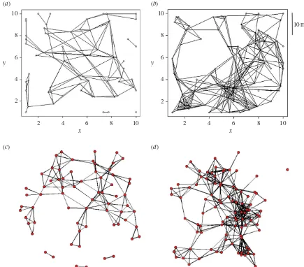
The 128 networks varied dramatically in size from 11 to 264 nodes. The networks were typically well connected in the sense that there was usually a single large component and a small number of isolated nodes or very small components (see electronic supplementary material, figure S1). Two examples, both from KCS, are shown in figure 1, one derived from trapping in winter from 13 November 2001 to 20 January 2002 and the other from trapping in summer from 28 June 2002 to 26 July 2002 when vole density was higher. The same data are displayed as spatial graphs (figure 1a,b, each node has coor-dinates) and non-spatial graphs (figure 1c,d, spatial locations are ignored).
3.2. Basic graph measures
Scatter plots of the mean degree and the CV of the degree dis-tribution, versus estimated vole density, are shown for all sites in figures 2 and 3. Mean degree (figure 2) was positively corre-lated with estimated population size. For two of the four sites, a power relationship (wherekklis a saturating function of den-sity) performed better (as measured by adjustedR2) than a
linear relationship. The scatterplots of the CV at sites BHP and ROB (figure 3a,b) show that for vole densities larger than approximately 50 voles per hectare, the CV drops to values not much larger than 1. For the other two sites, PLJ and KCS, the scatterplots show an absence of points in the upper right triangle of the axes, indicating high values of the CV are not observed at high densities. For all sites, the scatterplots indicate there is more heterogeneity in numbers of contacts at lower densities than at higher densities (figure 3).
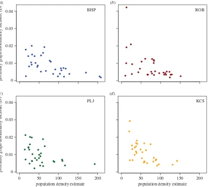
3.3. Proximity graph dissimilarity measures
Figure 4 and electronic supplementary material, figure S9, show that for all four sites the dissimilarity measures, D
andDu, tend to take lower values at higher vole population
densities, indicating that the networks tended to become closer to proximity graphs. All four scatterplots have an absence of points in the upper right triangle of the axes,
rsif.r
oy
alsocietypublishing.org
J.
R.
Soc.
Interfa
ce
12
:
20141004
indicating that at higher densities vole contacts tended to be more like what would be expected on the basis of proximity alone: voles were more likely to interact with others closest to them, rather than being ‘selective’ in their contacts. However, while there was an absence of high values at high densities, there was no such absence of low values at low densities, indicating that at low population density some contact net-works were very similar to proximity graphs and others were relatively dissimilar. The results for spatial variance quantified as distance deviation, a non-network measure of spatial restriction (see the electronic supplementary material), also show that voles reduce the spatial extent of their move-ments at higher densities (electronic supplementary material, figures S5 and S6). This is also consistent with the relation-ship between 1* and population density (see electronic supplementary material, figure S10) where again there is an absence of high values of1* at high population densities.
3.4. Model fitting
The values ofl—obtained when the model given by equation (2.5) was fitted to each of the 128 networks—were positively correlated with vole population density, indicating once again that the spatial scale over which voles were likely to interact with others decreased with density (see figure 5).
The relationship betweenlandDis shown in electronic sup-plementary material, figure S8. The values of l when the same statistical model that was fitted for the observed net-works was fitted to 100 equivalent random netnet-works were substantially less than the estimatedlvalue for the observed network: the average estimatedlfor the equivalent random networks was 0.36 (s.d. 0.022) while the l for the actual network was 1.69.
The results of the model fitting for the set of networks derived from site KCS and having at least 50 nodes are shown in table 1. The relative performance of the four models is measured using AICc. There is a uniformly sharp drop in AICc for model 1 compared with model 0, indicating strong support from the data for spatial proximity of nodes determining edges in these networks. For the majority of the networks, there was support for model 2 or 3 over model 1, and more often support for model 3 over model 2. Of the nine networks where model 1 had the greatest support, seven provided near-equivalent support for a more complex model (DAICc,2): five for model 3 and two for model 2. Over-all, therefore, there was support for the good-get-richer models that allowed large males, small males and females to differ in their overall propensity for contact (model 2) or in the degree to which distance discouraged contact (model 3). More often it was the latter. This overall picture was consistent across the 10
8
6
4
2
2 4 6 8 10
y
10
8
6
4
2 y
x
2 4 6 8 10
x
10 m (b)
(a)
[image:5.595.78.513.42.424.2](c) (d)
Figure 1.
Spatial and non-spatial plots of two of the 32 contact networks inferred from trapping sessions conducted at the Kielder Site (KSC) during (
a
) winter
(from 13 November 2001 to 20 January 2002) and (
b
) summer (from 28 June 2002 to 26 July 2002). The non-spatial versions of these networks, (
c
) and (
d
),
respectively, are produced in the software package R where there is an attempt to more clearly display the structure of the networks by minimizing the number of
edge-crossings. (Online version in colour.)
rsif.r
oy
alsocietypublishing.org
J.
R.
Soc.
Interfa
ce
12
:
20141004
four sites. When the data were pooled at the site level and a GLM similar to models 2 and 3 (see the electronic supplemen-tary material) was fitted to the data all factors were highly significant, providing further evidence that the three categories of voles that we identified (female, small male and large male) are behaving differently and these behavioural differences do further explain the absence or presence of edges in the networks.
When the edge data of all 128 networks was pooled the effect of density on the slope of the model and the effect of site on the intercept were both highly significant (see the electronic supplementary material). The results also show that the vole populations at two of the sites, ROB and BHP, perceive distance in more similar ways than any other pair-ing. Interestingly, the two similar sites are also those for which there was evidence that mean degree was a saturating function of population density.
Finally, the fitted good-get-richer model 3 indicated that for 19 of the networks large males were less discouraged by distance than either small males or females, and for the remaining four networks the small male class was the least discouraged by distance. On these same four occasions, the results for model 2 indicated that the small males had an overall greater propensity for contact. The female class was always the most discouraged by distance and almost
always had the lowest propensity for contact (there were two exceptions).
4. Discussion
Overall, the results for our field vole system suggest that as population density increases, the mean numbers of contacts, kkl, increases, and also that for at least two of the sites this increasing function saturates at the highest densities. In par-allel with this, as density increases, voles are more likely to interact simply with those closest to them (lower values of
D and Du) and the scale of spatial constraint increases
(higher values of l). We emphasize that l and the graph dissimilarities measure different things—the parameter l
indicates the degree to which distance between voles acts as a deterrent for contact whileDandDuindicate the similarity to a proximity graph without specifying that1be small or large—though in this datasetl andDare tightly related at higher densities and more loosely related for lower densities (see electronic supplementary material, figure S8). There was an absence of high values oflat low values of vole density, indicating voles always took advantage of the ‘extra’ space, but this spreading out sometimes meant low values of D and sometimes not. At high vole densities though, the contact (a)
(d) (c)
(b) BHP
5
4
3
2
1
0
ROB
PLJ KCS
mean degree
5
4
3
2
1
0
0 50 100 150 200
mean degree
–0.7025 + 0.3825x0.4604
–0.458 + 0.2136x0.5513
population density estimate
0 50 100 150 200
population density estimate 0.4264 + 0.0222x
[image:6.595.84.516.41.425.2]0.5802 + 0.0232x
Figure 2.
The mean degree of each of the 32 networks, from each of the four sites, plotted against estimated population density. A linear function and a power
function were fitted to the data separately for each site. In (
a
,
b
), for BHP and ROB, a power function was a better fit (adjusted
R
2values were, respectively, 0.669
versus 0.427 and 0.778 versus 0.642), while in (
c
,
d
), for PLJ and KCS, a linear function was the better fit (adjusted
R
2values were, respectively, 0.783 versus 0.6689
and 0.7308 versus 0.6907). (Online version in colour.)
rsif.r
oy
alsocietypublishing.org
J.
R.
Soc.
Interfa
ce
12
:
20141004
networksalwaysbecame close to proximity graphs. They also became ‘tighter’ proximity graphs (lower values of1*), with average distance deviation displaying much the same pattern as the other measures of spatial constraint.
The consistency of the relationships between the measures of spatial constraint and population density together paint a convincing picture that vole territories are shrinking with population density and becoming more strictly adhered to. The two dissimilarity measuresD andDuboth capture this effect. For this dataset, there in fact appears to be little difference between the two. Hence, while the underlying logic for the weighted version of the dissimilarity measure might be attractive, the additional complexity introduced by the weighting may be unnecessary.
The results here on contact rates increasing with density, but saturating at higher densities, are consistent with the find-ings of Smithet al. [18], and later Huet al. [19], who worked with infection data from the same four natural populations of field voles over the same time period for cowpox virus, a patho-gen transmitted by direct contact. We note that the contact networks we analyse are derived from trapping data and hence edges between individuals do not indicate direct contact, only that they shared the same trap at least once. The networks, therefore, are arguably most relevant to indirectly transmitted pathogens rather than directly transmitted pathogens such as cowpox. The correlation between indirect and direct contacts
between voles is hard to predict and may depend on the age and sex of the animals involved. While two voles that share the same space are more likely to come into direct contact, behaviour will play an important role and some animals may actively avoid each other. However, the similarity between the results here and from studies of cowpox transmission may suggest that in this system there is a broad positive corre-lation between indirect and direct contacts, with both showing a similar relationship with density. Smithet al. [18] estimated the relationship between density and direct host contact rate by fitting the output of differential equation models to time-series data on cowpox virus infection. They concluded that the contact rate over the year as a whole is a saturating function of field vole density, best modelled as intermediate between density- and frequency-dependence.
Smith et al. [18] further noted that such nonlinearity is consistent with a variety of plausible mechanisms, such as heterogeneity in the host–contact network (with a higher pro-portion of low-contact hosts at higher densities), or the limiting time available for contacts to be made (such that contact rate cannot keep pace with increasing density), or simply changes in the behaviour of individuals with population density (e.g. with individuals becoming more territorial at higher densities, and only contacting those on territory borders). One key benefit of studies such as those conducted here is that they may shed light on the mechanistic (individual-level) basis for (a)
(d) (c)
(b)
BHP 4
3
2
1
ROB
PLJ KCS
0 50 100 150 200
population density estimate
0 50 100 150 200
population density estimate
coefficient of variation
4
3
2
1
[image:7.595.91.513.40.425.2]coefficient of variation
Figure 3.
The CV (the standard deviation of the degree sequence scaled by the average degree) of each of the 32 networks, from each of the four sites, plotted
against estimated population density. The CV tends to drop as population density increases. Consistent with the plots of mean degree shown in figure 2, the results
for sites BHP and ROB appear to show a similar pattern to each other, as does the pairing PLJ and KCS. (Online version in colour.)
rsif.r
oy
alsocietypublishing.org
J.
R.
Soc.
Interfa
ce
12
:
20141004
these population-level phenomena. In the present case, hetero-geneity in contact rate decreased rather than increased at higher densities and so is unlikely to have contributed to the saturating curve. Our analysis adds nothing to considera-tions of time limitation, but we believe that the nature of vole contacts, passing one another in shared runways in the grass, itself makes it unlikely that they ever reach a position where there is simply no more time for further contact with con-specifics. The tendency, however, for voles to make contacts throughout the population at lower densities does indeed make it likely, when density is low, that contact rate will increase with density: the classic basis for density-dependent trans-mission [25]. Whereas space-constrained contacts at higher densities are akin to territorial behaviour and the consequent tendency to contact only territorial neighbours, whose numbers are relatively independent of density overall (classic frequency-dependence). Our results therefore suggest that the transmission function lying ‘between’ density- and frequency-dependence selected by the analysis in Smithet al. [18] is generated by con-tacts being closer to density-dependence at low densities and closer to frequency-dependence at high densities.
Even so, while a transition to frequency-dependence might be a good description of how thenumbersof contacts changes with density, the tendency to contact only territorial neighbours implies that thespatial distributionof contacts also changes with density. At higher densities then, there is a more severe departure
from the random-mixing assumption that underpins the dif-ferential equation models used by Smithet al. [18]. As spatial constraints on contacts increase there will be a stronger local saturation effect: infected individuals will be more often surrounded by recovered or already infected individuals. Hence, part of the explanation for the ‘transitioning’ phenomena at the population level may be that the fitted differential equation models underestimate the contact rate (as a function of density) in order to avoid overestimating the force of infection on the remaining susceptible portion of the population.
As well as the mean number of contacts increasing with population density, we observed that the level of individual variation in contact rate also decreases. It is well known that the variance of the degree distribution of a contact net-work enters calculations for the basic reproduction number in a nonlinear way, and that
R0¼r0 1þkk
2l
kkl2
,
wherer0is defined to be the basic reproduction number if there
was no heterogeneity in the numbers of contacts, and where the sharp brackets represent averages over the degree distri-bution,P(k) [9]. Note that this equation does not take into account the effects of any clustering in the network and the quantitykk2l=kkl2is the CV of the degree distribution. For the field vole populations, the data show thatr0increases with
(a) (b)
(c) (d)
BHP 0.04
0.03
0.02
0.01
0
ROB
PLJ KCS
proximity graph dissimilarity measure (
D
)
0.04
0.03
0.02
0.01
0
proximity graph dissimilarity measure (
D
)
0 50 100 150 200
population density estimate
0 50 100 150 200
[image:8.595.89.512.42.422.2]population density estimate
Figure 4.
The results for the dissimilarity measure,
D
, quantifying the difference between an observed spatial graph and the family of proximity graphs based on
the underlying point pattern. The values of
D
for the 32 networks from each site are plotted against estimated population density. The same pattern, that the
observed graphs tend to become more similar to proximity graphs as network size increases, is replicated at each site. (Online version in colour.)
rsif.r
oy
alsocietypublishing.org
J.
R.
Soc.
Interfa
ce
12
:
20141004
density (owing to increases in the average number of contacts) and hence R0 too, but two other things also happen that
would reduceR0 or reduce the force of infection on the
sus-ceptible part of the population: (i) the CV decreases (the networks become increasingly homogeneous), and (ii) the net-works become more spatial. Hence, our data imply that there may be a cancellation effect forR0, and more generally for
patho-gen transmission, whereby an increase in contact rate (and hence increase in transmission) owing to higher densities is at least par-tially ‘cancelled out’ by a decrease in individual heterogeneity and an increase in the spatial constraints on the contacts of the voles. This would predict that the spread of pathogens on these vole contact networks could be relatively insensitive to fluctuations in host density, and hence suggests an additional hypothesis as to why abundance thresholds operating in wildlife disease systems are rarely detected [26].
The good-get-richer models which divided the population into a large male class, a small male class and a female class were broadly supported by the vole data and suggested mature males were more likely to make contact with conspeci-fics than other groups of voles. The four networks (from KCS) for which this was not true show that the small male class instead had the greatest propensity for contact and was less constrained by distance. These networks may correspond to trapping at times of the year where young males are dispers-ing and seekdispers-ing to establish their own territory. Overall,
these patterns add to the growing number suggesting that large males may be particularly important in the transmission of infection because they are ‘super-contactors’ (e.g. [7]).
Data for determining animal contact networks are collected through a wide range of techniques (for a review see [3]), but most often animals must be captured and tagged, meaning that the contacts observed are between animals based within the same finite area. Hence, datasets will inevitably exclude long-range contacts that arise, for example, from dispersal move-ments of maturing animals, and are unlikely to include contacts with nomadic individuals moving through the study area, tend-ing to overestimate spatial constraints. However, Craftet al. [2] concluded that for the network of Serengeti lions, the presence of nomadic individuals had marginal epidemiological impact, especially for pathogens with short infectious periods. This sup-ports our contention that even with rare long distance events, spatial analyses of contact networks are worthwhile and spatial constraints may play an important role.
The results here suggest that we stand to gain three things from constructing well-defined network measures of spatial constraint. First, we are able to infer that our animal contact networks are indeed spatial. Values ofDandlcan be com-pared with networks from randomized equivalent trapping data to show that the observed network has significantly higher values (it is necessary to randomize the trapping data, rather than the edges of the observed network, if trap (a)
(d) (c)
(b)
spatial constraint (
l
)
BHP 2.5
2.0
1.5
1.0
spatial constraint (
l
)
2.5
2.0
1.5
1.0
ROB
PLJ KCS
r= 0.7702
r= 0.3997
r= 0.6623
r= 0.7713
0 50 100 150 200
population density estimate
0 50 100 150 200
[image:9.595.88.514.44.413.2]population density estimate
Figure 5.
The model parameter
l
(see Material and methods) which represents the strength of spatial constraints on contact rates between voles, were estimated
for each of the 32 networks from each of the four sites and plotted against estimated population density. The results for the four sites are consistent and show a
positive correlation. Pearson product – moment correlation coefficients are given as insets. (Online version in colour.)
rsif.r
oy
alsocietypublishing.org
J.
R.
Soc.
Interfa
ce
12
:
20141004
locations are used to allocate individuals a spatial position anddefine edges). Second, we gain a means of quantifying differences between two or more contact networks and so a basis for comparing different sites, species or times of year. Third, the measures lay the basis for mathematical descrip-tions of wildlife contact networks which could be used to generate theoretical networks representing host populations at much larger spatial scales, more relevant to real wildlife populations.
Data accessibility.The authors are happy to make the original data avail-able to others. Contact either M.B. (mbegon@liv.ac.uk) or S.T. (s.telfer@abdn.ac.uk).
Acknowledgements.We thank Kathy Horadam for useful discussions about the graph dissimilarity measures and Meggan Craft for reading an early draft of the manuscript and for her helpful advice and encouragement.
Funding statement.This work was partly supported by the Australian Research Council, grant no. DP120101188. Data collection was sup-ported by funding from NERC (GR3/13051) and the Wellcome Trust (075202/Z/04/Z).
References
1. Bohm M, Hutchings MR, White PCL. 2009 Contact networks in a wildlife-livestock host community: identifying high-risk individuals in the transmission of bovine TB among badgers and cattle.PLoS ONE
4, e5016. (doi:10.1371/journal.pone.0005016) 2. Craft ME, Volz E, Packer C, Meyers LA. 2011 Disease
transmission in territorial populations: the small-world network of Serengeti lions.J. R. Soc. Interface
8, 776 – 786. (doi:10.1098/rsif.2010.0511)
3. Craft ME, Caillaud D. 2011 Network models: an underutilized tool in wildlife epidemiology?
Interdiscip. Perspect. Infect. Dis.2011, 676949. (doi:10.1155/2011/676949)
4. Drewe JA, Eames KTD, Madden JR, Pearce GP. 2011 Integrating contact network structure into tuberculosis epidemiology in meerkats in South Africa: Implications for control.Prevent. Vet. Med.101, 113–120. (doi:10. 1016/j.prevetmed.2011.05.006)
5. Hamede RK, Bashford J, McCallum H, Jones M. 2009 Contact networks in a wild Tasmanian devil (Sarcophilus harrisii) population: using social network analysis to reveal seasonal variability in social behavior and its implications for transmission of devil facial tumour disease.Ecol. Lett.12, 1147– 1157. (doi:10.1111/j.1461-0248.2009.01370.x)
[image:10.595.44.554.124.506.2]6. Fenner AL, Godfrey SS, Bull CM. 2011 Using social networks to deduce whether residents or dispersers
Table 1.
AICc values for the four statistical models fitted to networks consisting of at least 50 individuals, for the site KCS. Model 0 represents the simplest
case wherein the rate of contact is the same constant value (see equation (2.1)) for all pairs of individuals, equivalent to the random-mixing assumption. Model
1 represents a simple model wherein the rate of contact decreases with distance between individuals. Models 2 and 3 are similar, respectively given by
equations (2.5) and (2.6) in the main text, both allow the parameters of Model 1 to vary between small males, large males and females, thus accounting for
some heterogeneity in the vole population. The lowest AICc value is highlighted in boldface, as well as any other AICc values for which the difference in AICc
from that for the best model is less than 2.
network
no.
voles
model 0
(constant)
model 1
(spatial)
model 2
(spatial
1
heterogeneity1)
model 3
(spatial
1
heterogeneity2)
2
50
589
327
329
327
3
84
1105
625
628
624
4
65
1008
582
579
571
6
87
256
145
148
137
7
149
2459
1282
1279
1275
8
124
2825
1369
1358
1352
9
141
2621
990
991
991
10
125
1149
529
530
525
11
164
3124
1432
1407
1386
12
242
3527
1740
1726
1718
13
219
6659
3234
3203
3208
14
232
5208
1970
1969
1969
15
141
1967
770
768
762
18
64
403
202
184
187
23
96
614
339
326
335
24
141
2754
1589
1527
1517
25
107
2107
944
944
935
26
81
707
334
338
336
28
77
1272
742
736
740
29
98
407
245
245
252
30
135
1449
856
854
858
31
98
1043
459
461
459
32
69
518
293
295
296
rsif.r
oy
alsocietypublishing.org
J.
R.
Soc.
Interfa
ce
12
:
20141004
spread parasites in a lizard population.J. Anim. Ecol.80, 835 – 843. (doi:10.1111/j.1365-2656.2011. 01825.x)
7. Perkins SE, Cagnacci F, Stradiotto A, Arnoldi D, Hudson PJ. 2009 Comparison of social networks derived from ecological data: implications for inferring infectious disease dynamics.J. Anim. Ecol.78, 1015 – 1022. (doi:10.1111/j.1365-2656.2009.01557.x) 8. Porphyre T, McKenzie J, Stevenson MA. 2011
Contact patterns as a risk factor for bovine tuberculosis infection in a free-living adult brushtail possumTrichosurus vulpeculapopulation.Prevent. Vet. Med.100, 221 – 230. (doi:10.1016/j.prevetmed. 2011.03.014)
9. May RM. 2006 Network structure and the biology of populations.Trends Ecol. Evol.21, 394 – 399. (doi:10.1016/j.tree.2006.03.013)
10. Mollison D. 1977 Spatial contact models for ecological and epidemic spread.J. R. Stat. Soc. B
39, 283 – 326.
11. Keeling MJ. 1999 The effects of local spatial structure on epidemiological invasions.Proc. R. Soc. Lond. B266, 859 – 867. (doi:10.1098/rspb. 1999.0716)
12. Caldarelli G, Capocci A, De Los Rios P, Munˇoz MA. 2002 Scale-free networks from varying vertex intrinsic fitness.Phys. Rev. Lett.89, 258702. (doi:10. 1103/PhysRevLett.89.258702)
13. Davis S. 2011 Percolation on a spatial network with individual heterogeneity as a model for disease spread among animal host populations. In
Sustaining our future: understanding and living with
uncertainty(eds F Chan, D Marinova, RS Anderssen), pp. 905 – 911. Perth, Australia: Modelling and Simulation Society of Australia and New Zealand (19th International Congress on Modelling and Simulation).
14. Volz EM, Miller JC, Galvani A, Meyers LA. 2011 Effects of heterogeneous and clustered contact patterns on infectious disease dynamics.PLoS Comput. Biol.7, e1002042. (doi:10.1371/journal. pcbi.1002042)
15. Davis S, Begon M, De Bruyn L, Ageyev VS, Klassovskiy NL, Pole SB, Viljugrein H, Stenseth NC, Leirs H. 2004 Predictive thresholds for plague in Kazakhstan.Science304, 736 – 738. (doi:10.1126/ science.1095854)
16. Davis S, Trapman P, Begon M, Leirs H, Heesterbeek JAP. 2008 The abundance threshold for plague as a critical percolation phenomenon.Nature454, 634 – 637. (doi:10.1038/nature07053) 17. Turner J, Begon M, Bowers RG. 2003 Modelling
pathogen transmission: the interrelationship between local and global approaches.Proc. R. Soc. Lond. B270, 105 – 112. (doi:10.1098/rspb.2002. 2213)
18. Smith MJ, Telfer S, Kallio ER, Burthe S, Cook AR, Lambin X, Begon M. 2009 Host-pathogen time series data in wildlife support a transmission function between density and frequency dependence.Proc. Natl Acad. Sci. USA106, 7905 – 7909. (doi:10.1073/pnas.0809145106) 19. Hu H, Nigmatulina K, Eckhoff P. 2013 The scaling of
contact rates with population density for the
infectious disease models.Math. Biosci.244, 125 – 134. (doi:10.1016/j.mbs.2013.04.013) 20. Lambin X, Petty SJ, MacKinnon JL. 2000 Cyclic
dynamics in field vole populations and generalist predation.J. Animal Ecol.69, 106 – 118. (doi:10. 1046/j.1365-2656.2000.00380.x)
21. Begon M, Telfer S, Burthe S, Lambin X, Smith MJ, Paterson S. 2009 Effects of abundance on infection in natural populations: field voles and cowpox virus.
Epidemics1, 35 – 46. (doi:10.1016/j.epidem.2008. 10.001)
22. Dale MRT, Fortin M-J. 2010 From graphs to spatial graphs.Annu. Rev. Ecol. Evol. Syst.41, 21 – 38. (doi:10.1146/annurev-ecolsys-102209-144718) 23. R Core Team. 2013R: a language and environment
for statistical computing. Vienna, Austria: R Foundation for Statistical Computing. (http://www. R-project.org/)
24. Press WH, Teukolsky SA, Vetterling WT, Flannery BP. 2007Numerical recipes: the art of scientific computing, 3rd edn. New York, NY: Cambridge University Press.
25. Begon M, Bennett M, Bowers RG, French NP, Hazel SM, Turner J. 2002 A clarification of transmission terms in host-microparasite models: numbers, densities and areas.Epidemiol. Infect.129, 147 – 153. (doi:10.1017/S0950268802007148) 26. Lloyd-Smith JO, Cross PC, Briggs CJ, Daugherty M,
Getz WM, Latto J, Sanchez MS, Smith AB, Swei A. 2005 Should we expect population thresholds for wildlife disease?Trends Ecol. Evol.20, 511 – 519. (doi:10.1016/j.tree.2005.07.004)