Design and implementation of a remotely accesible inrush current testing package for power (distribution)transformers

(1)

Faculty of Engineering and Surveying

DESIGN AND IMPLEMENTATION OF A

REMOTELY ACCESSIBLE INRUSH CURRENT

TESTING PACKAGE FOR POWER

(DISTRIBUTION) TRANSFORMERS

A dissertation submitted by

Glenn SPRINGALL

In fulfillment of the requirements of

Courses ENG4111 and 4112 Research Project

towards the degree of

Bachelor of Engineering (Electrical/Electronic) and Bachelor Science

(Chemistry)

(2)

ABSTRACT

Inrush current or surge current in Power (distribution) transformers has been known to exist since transformers were first designed and manufactured. Since that time, the phenomenon has been researched, modelled and factored into designs.

(3)

University of Southern Queensland

Faculty of Engineering and Surveying

ENG4111 Research Project Part 1 &

ENG4112 Research Project Part 2

LIMITATIONS OF USE

The Council of the University of Southern Queensland, its Faculty of Engineering and Surveying, and the staff of the University of Southern Queensland, do not accept any responsibility for the truth, accuracy or completeness of material contained within or associated with this dissertation.

Persons using all or any part of this material do so at their own risk, and not at the risk of the Council of the University of Southern Queensland, its Faculty of Engineering and Surveying or the staff of the University of Southern Queensland.

This dissertation reports an educational exercise and has no purpose or validity beyond this exercise. The sole purpose of the course "Project and Dissertation" is to contribute to the overall education within the student’s chosen degree programme. This document, the associated hardware, software, drawings, and other material set out in the associated appendices should not be used for any other purpose: if they are so used, it is entirely at the risk of the user.

Professor Frank Bullen Dean

(4)

CERTIFICATION

I certify that the ideas, designs and experimental work, results, analyses and conclusions set out in this dissertation are entirely my own effort, except where otherwise indicated and acknowledged.

I further certify that the work is original and has not been previously submitted for assessment in any other course or institution, except where specifically stated.

Glenn William Springall Student Number: 0050026015

_____________________________ Signature

(5)

ACKNOWLEDGEMENTS

This research was carried out under the principle supervision of Dr Tony Ahfock. His support, knowledge and assistance have been vital in maintaining accurate and reliable research.

I would also like to acknowledge and thank Mr Don Gelhaar, USQ technical staff for laboratory assistance, Mr Vikram Kapadia for SCADA and PLC assistance.

(6)

CONTENTS

ABSTRACT... I LIMITATIONS OF USE ...II CERTIFICATION ... III ACKNOWLEDGEMENTS ... IV CONTENTS...V LIST OF FIGURES ...VII LIST OF TABLES ...VIII LIST OF TABLES ...VIII GLOSSARY ... IX

CHAPTER 1: INTRODUCTION ... 1

1.1 Justification for the Project ... 1

1.2 Dissertation Outline ... 1

CHAPTER 2: LITERATURE REVIEW ... 3

2.1 Overview of Inrush Current ... 3

2.2 Consequences of Inrush Current ... 7

2.3 Modern Techniques for combating Inrush Current ... 8

2.4 Application of Electronic Differential Relays in Protection Systems ... 9

CHAPTER 3: METHODOLOGY ... 13

3.1 Project Aims and Objectives... 13

3.2 Methodology of Objectives... 14

CHAPTER 4: FUNCTIONALITIES OF THE DIFFERENTIAL RELAY ... 17

4.1 Purpose and Functions of a Current Differential Relay... 18

4.2 SEL-387A Protection Relay setting guide ... 20

4.3 Current System Settings... 40

CHAPTER 5: INRUSH CURRENT MATHEMATICAL MODELING ... 41

5.1 Mathematical Modeling Purpose ... 41

5.2 Harmonics existing in inrush current ... 41

5.3 Differential relay discrimination against Inrush Current ... 44

CHAPTER 6: INRUSH CURRENT TEACHING PACKAGE ... 45

6.1 Inrush Current Theory... 46

6.2 PLC and SCADA set up ... 50

6.3 Test Rack Setup for Inrush Current observation... 52

6.4 Inrush Current Observation Activity ... 54

6.5 Summary and Conclusions ... 57

6.6 Review Questions and Answers... 58

(7)

7.1 Future Works to be undertaken... 60

7.2 Advantages of Future Works ... 61

CHAPTER 8: SUMMARY AND CONCLUSIONS ... 63

8.1 Summary of Achievements... 63

8.2 Conclusion ... 64

REFERENCES ... 65

BIBLIOGRAPHY... 66

APPENDICES ... 70

Appendix A- Project Specification ... 70

Appendix B- Relay Setting Sheets for the SEL-387A as at 28 October 2008 ... 71

(8)

[image:8.612.89.524.122.504.2]

LIST OF FIGURES

Figure 1 - Transformer Model No-Load ... 3

Figure 2 - Steady State Voltage and Magnetic Flux Waveforms ... 4

Figure 3 - Transformer Hysterisis Loop ... 5

Figure 4 - Voltage Applied to Primary Side of Transformer... 6

Figure 5 - Current Response to Input Voltage ... 6

Figure 6 - Internal design of a power transformer ... 7

Figure 7 - Simplistic Differential Protection Schematic... 10

Figure 8 - Front and Rear view of the SEL-387A Relay ... 18

Figure 9 - Three Phase Energisation of a test transformer (Current)... 42

Figure 10 - Stem Plot of the harmonics in each phase... 43

Figure 11 - Transformer Model No-Load ... 46

Figure 12 - Steady State Voltage and Magnetic Flux Waveforms ... 47

Figure 13 - Transformer Hysterisis Loop ... 48

Figure 14 - Voltage Applied to Primary Side of Transformer... 49

Figure 15 - Current Response to Input Voltage ... 49

Figure 16 - PLC Ladder Diagram for the Circuit Breaker... 51

Figure 17 - SCADA interface to the test rack system... 52

(9)

LIST OF TABLES

(10)

GLOSSARY

USQ University of Southern Queensland PLC Programmable Logic Controller

SCADA Supervisory Control and Data Acquisition EMF Electromotive Force

CB Circuit Breaker

CT Current Transformer

OC Overcurrent

REF Restricted Earth Fault LED Light Emitting Diode

PPE Personal Protective Equipment SEF Sensitive Earth Fault

AR Autoreclose

(11)

CHAPTER 1: INTRODUCTION

1.1

Justification for the Project

It is important that Electrical Engineers and Electrical Scientists alike, understand how and why a transformer works. It is important that they understand where losses occur, what those losses look like and what faults can occur inside and outside a transformer. This understanding is crucial if the industry is to see an increase in “SMART” transformers, to develop more energy efficient transformers, to increase transformer capacities and also to reduce the physical size of transformers.

This particular project investigates the inrush current phenomenon associated with the energisation of transformers, particularly power transformers. Much work has been completed in the past two hundred years to analyse transformers and their operation. This project aims to confirm those assumptions and findings through mathematical analysis of an inrush current test rack facility. Through this investigation the aims are to provide a resource for academics to use in creation of a well balanced, practical and theoretical course on either transformers or protection systems.

1.2

Dissertation Outline

The second chapter of this dissertation focuses on the background of inrush current. It explores the place that inrush current has in the power industry, particularly in transformer technologies and the effects and limitations on transformer designs. The chapter also covers some background information on how sequential switching and “SMART” relays are employed to combat nuisance tripping from high inrush currents.

Chapter three covers the methodologies used to achieve the project aims and objectives.

(12)

Chapter 1 Introduction

details the appropriate way to set a differential relay to avoid inrush current tripping including second and fourth harmonic analysis.

Chapter five details the mathematics underpinning inrush current. Inrush current is analysed from the three phase example to determine the levels harmonic present using MATLAB.

The sixth chapter focuses on the teaching module of inrush current. This includes a theoretical component, a mathematical analysis component, a relay setting component, a practical component and then concluded by review questions.

Chapter seven outlines what works could be undertaken in the future that associate with this project. Details of the cost and benefit of conducting these works are also mentioned.

(13)

CHAPTER 2: LITERATURE REVIEW

2.1

Overview of Inrush Current

The problems associated with inrush current and the possible solutions and management of the high currents have been available for many years. It is very well known that the cause of inrush current is due to a combination of magnetic flux and part cycle voltage.

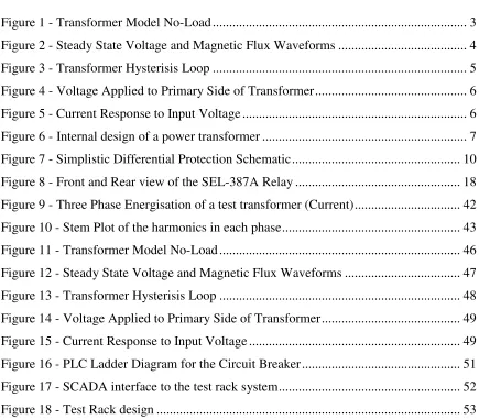
[image:13.612.90.460.335.555.2]

Figure 1 shows a simple transformer diagram of the primary windings (ie no load). In the diagram, v represents the voltage of EMF of the windings, i represents the primary side current, N represents the number of turns (of the windings) and x is a switch.

Figure 1 - Transformer Model No-Load

For this transformer model it is known that the voltage, V is directly proportional to the number of turns by the change in magnetic flux over the change in time. As represented by the below formula.

t

N

V

∂

(14)

Chapter 2 Literature Review

Where magnetic flux is represented by phi = Φ, number of turns =N, voltage=V and the time =t.

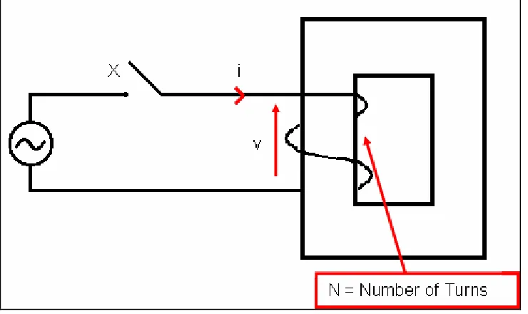
[image:14.612.90.484.276.588.2]

This model demonstrates that at steady state (ie when the transformer is operating under normal conditions after a long continuous period), that the voltage and magnetic flux are directly proportional. Subsequently the voltage and the current are also directly proportional. This can be shown as a representation of two waveforms, a voltage waveform and a magnetic flux waveform. Where Voltage=Sin(ωt) and Magnetic Flux=Cos(ωt) and is seen in figure 2.

(15)

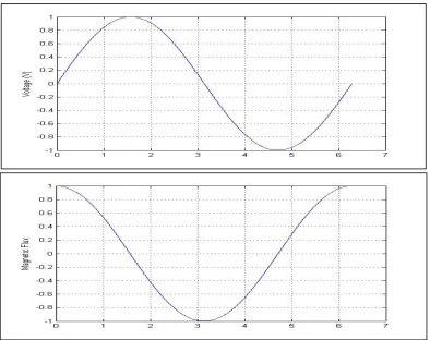
Using Ohm’s law, current can be calculated by using the number of turns and the magnetic flux so that current becomes proportional to NΦ as per the below formula.

i

α

N

Φ

[image:15.612.99.473.301.495.2]

This relationship, in a perfect situation would behave in a linear fashion. However the real relationship between current and magnetic flux is in a hysterisis loop arrangement. A real hysterisis loop of a test transformer at the University of Southern Queensland, performed by Dr Tony Ahfock, can be seen in figure 3. This diagram shows that the magnetic flux versus the current in a transformer does not follow a linear relationship but rather forms an envelope, hysterisis arrangement. It can also be seen that when the flux is very high, current can be tending towards infinitely high (shown by the flat line at the top of the hysterisis loop).

Figure 3 - Transformer Hysterisis Loop

Dr Tony Ahfock (USQ), along with students, has performed many tests on single and three phase transformers, analyzing the inrush current phenomenon. Figure 4 shows one such energisation. It can be seen in the diagram that the transformer has voltage applied to the primary side at approximately 0.052 seconds. It can also be seen that the time which the voltage is applied to the transformer is almost half way through one cycle of the AC voltage waveform. Additional information from the waveform is that the applied voltage is approximately 600Vpeak.

N

Φ

(16)

[image:16.612.105.493.77.246.2]

Figure 4 - Voltage Applied to Primary Side of Transformer

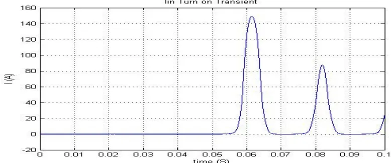
The corresponding current waveform is shown in Figure 5. In this diagram, two clear decaying peaks can be seen, with a third slightly obscured. The diagram also shows the current drawn reaching approximately 150A which is well above the rated current of this transformer. The first peak is delayed by approximately 0.01 seconds due to the lagging nature of the current. If this waveform was run till steady state, a smooth cosine shaped curve centered about the x-axis would be visible.

[image:16.612.108.497.437.600.2]

(17)

2.2

Consequences of Inrush Current

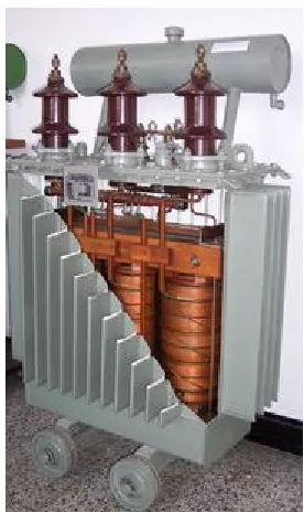
[image:17.612.236.374.356.588.2]

Inrush current can have an adverse affect to the internal mechanical stresses exerted upon a transformer winding. The internal construction of a transformer is shown in Figure 6. It can be seen that within the transformer there exists many mechanical devices to support the transformer such as bolts, wedges and pre-pressed bandages. Stuerer and Frohlich (2002) found that, the design of these mechanical support structures is determined by the highest possible current peak which normally occurs under a short circuit condition. However the results of their study showed that inrush current peaks of approximately 70% of the rated short circuit current caused the same magnitude force as those at short circuit. Their study has also shown that although inrush currents normally are smaller than short circuit currents, the inrush current forces can be higher and for more extended periods of time.

Figure 6 - Internal design of a power transformer (http://en.wikipedia.org/wiki/Transformer

(18)

weakening the windings resulting in lower efficiency, or worst case, serious injury or death from an explosion of the windings.

2.3

Modern techniques for combating Inrush Current

Inrush current has been a factor of transformer design and switching for as long as the transformer has been in operation. Many techniques have been adopted and explored to understand the phenomenon and guard against the unhelpful results that inrush current has the potential to cause. The two most common techniques for minimising the effects of inrush current in power transformers are controlled switching and electronic relays. The third option, which is not as common in power transformers but is used commonly in switching power supplies, (Ametherm, http://www.ametherm.com/Inrush_Current/ inrush_ current_faq.html) is the thermistor.

(19)

prestrikes, it is very difficult to energise a transformer at a specific instant. For these reasons and for reasons of practicality, the controlled switching, utilising the relationship of the flux to voltage is rarely incorporated into design for Power applications.

Thermistors are a passive circuit component used in sensitive switching power supplies. The thermistor operates as a current limiting device that provides resistance relative to a thermal threshold. As a thermistor heats, due to the increase in current (from the inrush current), it slowly decreases in resistance until the thermistor is at thermal maximum and the resistance is minor in terms of the overall system. Obviously this application of inrush current, surge limiting is not practical in a power application due to the relative size the component would have to be to provide any noticeable decrease in the magnitude of inrush current.

Finally, Electronic Relays are the most common modern inrush current monitoring device. These electronic relays do not change the magnitude of the inrush current drawn. However, they do minimise the effect that the large current draw has on the rest of the system. This is done by real time analysis of the current as it passes through the relay. If a surge current is detected by the relay, an analysis of the current for second harmonics is conducted. If the surge contains large second harmonics, it is neglected for a period of up to ten cycles. This process allows the relay to operate correctly and not cause a nuisance trip each time the transformer is energised. Relays and their application to inrush current are discussed further in Section 2.4.

2.4

Application of Electronic Differential Relays in Protection

Systems

(20)

[image:20.612.60.556.72.338.2]

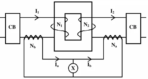
Figure 7 - Simplistic Differential Protection Schematic

Figure 7 shows that the differential protection system operates within the transformer circuit breakers. N1 and N2 represent the number of turns on the primary and secondary

side of the transformer. I1 and I2 represent the current coming into and the current

coming out of the transformer. Na and Nb represent the windings on the current

transformers (CT) that feed a “sample” or a “sniff” of the currents through the transformer by the currents Ia and Ib. The ratio of turns N1:N2 must be the same ratio, but

not the same number of turns, as Na:Nb. X represents a sensitive relay current sensor.

Put simply, when there is a fault inside the transformer (i.e. when what is going into the transformer is not coming out of the transformer) the CBs trip, isolating the transformer from the surrounding system and any source voltage and thus preventing any further damage. The system achieves this using the CTs at Na and Nb and the relative currents Ia

and Ib. When I1/I2 ≠ N2/N1, Ia≠Ib. Because the currents Ia do not equal Ib, current is

forced to flow in the branch containing the sensitive current sensing relay, X (Kirchhoff’s current law). The sensitive current relay is designed to detect any variance to its threshold and forces the circuit breakers to trip as mentioned.

CB

I

1

I

2

N

_b

N

₁

N

₂

N

a

I

a

I

b

(21)

At steady state or when the transformer is operating as normal, I1/I2 equals N2/N1 and

subsequently Ia equals Ib. Because Ia equals Ib there is negligible current flow through the

sensitive Current Sensing Relay and hence the circuit breakers will not trip.

The reason that differential protection is the cause of investigation is that inrush current, as described by Hunt, Schaefer and Bentert (2008), can cause a tripping of the differential protection systems as the relay believes it to be an internal fault. This type of tripping is regarded as a nuisance fault (for obvious reasons) and much despised amongst protection engineers in industry.

Protection Engineers have utilised many methods of avoiding nuisance tripping. One such method documented by Hunt, Schaefer and Bentert (2008) utilises and analyzes the current’s second harmonic. They recommend that an analysis of the current to be computed by the differential relay and if the current has a high level of second harmonics to allow the current to pass for a further typical two to three cycles. This allows the transformer to keep operating during an inrush current “fault” but to still trip if another type of fault presents itself.

Hong and Qin (2000) contradict the usefulness of the second harmonic to determine inrush current faults. This is based on findings that with the increase in underground cables and overall higher capacities of distribution networks, there is a natural increase in the second harmonic. This makes other types of faults indistinguishable to inrush current. They are recommending further work be done in utilizing a wavelet based discrimination method thus avoiding the second harmonic issues arising.

(22)

(23)

CHAPTER 3: METHODOLOGY

This chapter outlines the project aims, objectives and the methodologies employed to accomplish them.

3.1

Project Aims and Objectives

The project aims are detailed in the Project Specification in Appendix A. The primary aim of this project is to investigate the inrush current phenomenon from a mathematical point of view and report on the findings. Those findings should include references to magnetic flux densities, harmonics and the magnitudes of the resultant currents (inrush current).

The secondary aim of this project is to develop a training package that is suitable to be used as a teaching package at USQ. This teaching package should include all relevant inrush current theory, differential relay data, practical experimentation information and also a set of review questions and answers. This teaching package should be appropriate to be included into a course designed for teaching transformer theory or protection theory.

The following core project objectives have been developed for fulfillment in this project and are addressed throughout the dissertation:

• Research inrush current test characteristics of power transformers

• Discuss with industry professionals and academics, the main features that are to be included in a transformer inrush current test facility.

• Design and build a transformer inrush current test rack that can be PLC controlled

(24)

Chapter 3 Methodology

• Design and create the SCADA interface for the PLC and inrush current test environment

• Write full documentation on the design and operation the of the equipment suitable for use as a teaching course

• Develop and validate mathematical models to explain transformer inrush current

• Complete dissertation

3.2

Methodology of Objectives

Each of the Project aims has an associated methodology for completion.

3.2.1 Research Inrush Current test characteristics of Power Transformers

This objective is purely research based. To complete this objective, a thorough search of online, text based and journal sources needs to be conducted. Additionally the information and knowledge from USQ lecturers, specifically Dr Tony Ahfock, effectively is to be sourced and utilised in the completion of this objective.

3.2.2 Discuss with Industry Professionals and Academics, the main features

that are to be included in a transformer Inrush Current test facility.

(25)

3.2.3 Design and build a transformer Inrush Current Test rack that can be

PLC controlled

To complete this objective, the design features deemed appropriate from research and professionals is to be combined and drawn. The rack is to feature PLC control, Differential Relay Integration and remote access. Once the plans have been drawn, approval is to be sought for the construction of the test rack.

3.2.4 Program the PLC to conduct all Inrush Current test requirements

including the use of protection relays

To complete this objective, PLC programming tutorials are to be conducted. The programming is to be designed to perform all inrush testing actions including the incorporation of the differential relay. Discussions with post-graduate students will also need to be conducted to ensure that this objective is not being hindered by similar works.

3.2.5 Design and create the SCADA interface for the PLC and Inrush

Current test environment

To complete this objective, the PLC control is to be interfaced remotely through a SCADA panel. This SCADA programming will also require completion of a SCADA tutorial. Discussions with post-graduate students will also need to be conducted to ensure that this objective is not being hindered by similar works in the test rack environment.

3.2.6 Write full documentation on the design and operation of the equipment

suitable for use as a teaching course

(26)

Chapter 3 Methodology

phenomenon. Additionally the teaching module will provide review questions and answers.

3.2.7 Develop and validate mathematical models to explain transformer

inrush current

To achieve this objective, inrush testing will need to occur. When reproducible tests are completed, the data is to be analysed using MATLAB. The analysis to be conducted includes performing an Fast Fourier Transform (FFT) on the inrush current data to provide evidence for inrush current harmonics, determination of peak inrush current and also an approximation of the inrush current decay time.

3.2.8 Complete dissertation

(27)

CHAPTER 4: FUNCTIONALITIES OF THE

DIFFERENTIAL RELAY

(28)

Chapter 4 Functionalities of the Differential Relay

4.1

Purpose and Functions of a Current Differential Relay

As described in Chapter 2, the differential relay is a device that prevents damage to the asset (transformer) that its sensors are either side of. This is achieved through making an assumption that the current traveling into a transformer, after slight losses, must proportionally exit the asset.

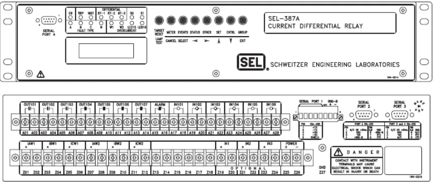
[image:28.612.91.525.380.565.2]

The differential relay that is the focus of this dissertation is the Schweitzer Engineering Laboratories, SEL-387A Current Differential and Overcurrent Protection Relay. This relay can protect assets such as transformers, buses, generators, reactors from current differentials, overcurrent and also temperature threshold protection. Additionally the relay has the capacity to be utilised as a restricted earth fault protection device. A front and rear view of this relay is shown in figure 8.

Figure 8 - Front and Rear view of the SEL-387A Relay

(29)

at reducing the damage due to severe faults, especially on power transformers. As well as providing the circuit break order, the relay records the system data such as current and phase angles leading up to and including the tripping of the circuit breaker. This makes the SEL-387A also useful in fault analysis and determining the source (based on the magnitude, phase and angle of the current) that caused the fault.

A differential relay of the nature described above is often referred to as a SMART relay due to their micro-processor control, but also because of the supplementary features they can offer a user. Some of these features include instantaneous phase and current measurements, peak demand data, circuit breaker information such as breaker wear and also battery monitoring (in some applications). The secondary reasoning for being termed “SMART” relays is that they can be interfaced using SCADA. This feature allows user to be remote of the relay’s location and still access the data and tripping notifications. Additionally the relay can be reset remotely allowing full operation of the relay and asset without a physical inspection NB this practice would not be employed every time due to Occupational Health and Safety policies regarding inspection of tripped assets to ensure no auxiliary issues are present or are the cause.

(30)

4.2

SEL-387A Protection Relay setting guide

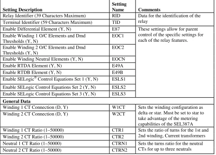
The SEL-387A protection relay has a multitude of settings that are inputted to ensure that the relay is correctly configured to operate on the specific asset that it is connected to. There are over 600 settable options on the SEL-387A relay to ensure correct operation. These settings range from naming the relay, setting the conditions of the LED indicators being lit to determining the number of turns on the current transformer (CT). Accurate and careful programming of the settings is paramount in efficient and correct operation of the relay.

[image:30.612.89.535.390.709.2]

Table 1 is a summary of operation for each of the relay settings. All of the associated logic diagrams for all of these settings can be found in the SEL-387A Differential Relay Instruction Manual.

Table 1: Summary of operation of each SEL-387A relay setting

Setting Description

Setting

Name Comments

Relay Identifier (39 Characters Maximum) RID

Terminal Identifier (59 Characters Maximum) TID

Data for the identification of the relay

Enable Differential Element (Y, N) E87

Enable Winding 1 O/C Elements and Dmd Thresholds (Y, N)

EOC1

Enable Winding 2 O/C Elements and Dmd Thresholds (Y, N)

EOC2

Enable Winding Neutral Elements (Y, N) EOCN

Enable RTDA Element (Y, N) E49A

Enable RTDB Element (Y, N) E49B

Enable SELogic® Control Equations Set 1 (Y, N) ESLS1

Enable SELogic Control Equations Set 2 (Y, N) ESLS2 Enable SELogic Control Equations Set 3 (Y, N) ESLS3

These settings allow for parent control of the specific settings for each of the relay features.

General Data

Winding 1 CT Connection (D, Y) W1CT

Winding 2 CT Connection (D, Y) W2CT

Sets the winding configuration as delta or star. Must be set to star to take advantage of the metering capabilities of the SEL387A

Winding 1 CT Ratio (1–50000) CTR1

Winding 2 CT Ratio (1–50000) CTR2

Sets the ratio of turns for the 1st and 2nd winding, Current transformers

Neutral 1 CT Ratio (1–50000) CTRN1

Neutral 2 CT Ratio (1–50000) CTRN2

(31)

Neutral 3 CT Ratio (1–50000) CTRN3 Maximum Power Xfmr Capacity (OFF, 0.2–5000.0

MVA)

MVA Sets the maximum power the

transformer would be subject to Define Internal CT Connection Compensation (Y, N) ICOM Allows for internal compensation for

the CT Winding 1 CT Conn. Compensation (0, 1, …, 12) W1CTC

Winding 2 CT Conn. Compensation (0, 1, …, 12) W2CTC

Relay vector shift and zero sequence compensation shifts for winding CT compensation

Winding 1 Line-to-Line Voltage (1.00–1000.00 kV) VWDG1 Winding 2 Line-to-Line Voltage (1.00–1000.00 kV) VWDG2

Set to the nominal voltage of the power transformer winding.

Differential Elements

Note: TAP1 and TAP2 are auto-set by relay if MVA setting is not OFF. Winding 1 Current Tap (0.10–31.00 A secondary) (1

A)

TAP1

Winding 2 Current Tap (0.10–31.00 A secondary) (1 A)

TAP2

These settings are auto-set via the Maximum Power Xfmr Capacity setting

Restrained Element Operating Current PU (0.10– 1.00 TAP)

O87P

Restraint Slope 1 Percentage (5–100%) SLP1

Restraint Slope 2 Percentage (OFF, 25–200%) SLP2 Restraint Current Slope 1 Limit (1.0–20.0 TAP) IRS1

These settings relate to the overall differential protection characteristics. The particular settings relate to the threshold of operation such that O87P is the minimum "operate" level for operation, SLP1 is the initial slope of the relay curve that begins at the origin and intersects O87P at IRT=O87P*100/SLP1. Also IRS1 is the limit of SLP1for operation (beginning of SLP2) and SLP2 is the second slope and must be equal to or greater that SLP1 for normal curve plotting.

Unrestrained Element Current PU (1–20 TAP) U87P This setting allows for quick reaction to very high currents that are obvious faults. This setting can be tripped by inrush, therefore needs to be set higher than expected inrush magnitude.

Second-Harmonic Blocking Percentage (OFF, 5– 100%)

PCT2

Fourth-Harmonic Blocking Percentage (OFF, 5– 100%)

PCT4

These settings directly relate to the discernment of inrush current due to inrush current having high values of 2nd and 4th harmonics. These settings are ratios of the second or fourth harmonic magnitude divided by the fundamental magnitude. Fifth-Harmonic Blocking Percentage (OFF, 5–100%) PCT5

Fifth-Harmonic Alarm Threshold (OFF, 0.02–3.2 TAP)

TH5P

Fifth-Harmonic Alarm TDPU (0.000–8000.000 cyc) TH5D

These settings relate to over-excitation. Over-excitation produces odd harmonics and PCT5 allows for the setting of the core flux density ratio. TH5P and TH5D allow for an alarm and pickup delay for these types of conditions.

DC Ratio Blocking (Y, N) DCRB This setting allows for the control of

(32)

Harmonic Restraint (Y, N) HRSTR This allows for the relay to detect the

second and fourth harmonics independently and on trip if the combination of both exceeds the sum threshold but not for 2nd or 4th harmonics independently.

Independent Harmonic Blocking (Y, N) IHBL Activates harmonic blocking on

phases independently that they are detected on, not for all three phases. Restricted Earth Fault

Enable 32I (SELogic control equation) E32I1 Enables REF1

Operating Quantity from Wdg. 1, Wdg. 2 (1, 2, 12) 32IOP1 Indicates which winding is being monitored

Positive-Sequence Current Restraint Factor, I0/I1 (0.02–0.50)

a01

Residual Current Sensitivity Threshold (0.05–3 A secondary) (1 A)

50GP1

Settings for the detection of the REF fault (1)

Enable 32I (SELogic control equation) E32I2 Enables REF2

Operating Quantity from Wdg. 1, Wdg. 2 (1, 2, 12) 32IOP2 Indicates which winding is being monitored

Positive-Sequence Current Restraint Factor, I0/I1 (0.02–0.50)

a02

Residual Current Sensitivity Threshold (0.05–3 A secondary) (1 A)

50GP2

Settings for the detection of the REF fault (2)

Winding 1 O/C Elements Winding 1 Phase O/C Elements

Phase Def.-Time O/C Level 1 PU (OFF, 0.05–20 A secondary) (1 A)

50P11P Relates to the definite time element of the O/C protection and is dictated by the SELogic 50Pn1TC equation as to whether currents of higher

magnitude than this setting should trip

Phase Level 1 O/C Delay (0.00–16000.00 cycles) 50P11D Relates to the operation of 50Pn1P in only allowing a trip if the magnitude of current that is above threshold is maintained for the entirety of the delay setting

50P11 Torque Control (SELogic control equation) 50P11TC The control equation for 50Pn1P Phase Inst. O/C Level 2 PU (OFF, 0.05–20 A

secondary) (1 A)

50P12P This setting relates to Instantaneous O/C element and is dictated by the torque-controlled SELogic 50PnTC equation as to whether the exceeded threshold constitutes a trip

secondary) (1 A)

50P13P

Phase Inst. O/C Level 4 PU (OFF, 0.05–20 A secondary) (1 A)

50P14P

These settings are non-torque controlled settings that are a simple monitoring of the phases to determined whether the magnitude has been exceeded

Phase Inv.-Time O/C PU (OFF, 0.10–3.20 A secondary) (1 A)

51P1P

Phase Inv.-Time O/C Curve (U1–U5, C1–C5) 51P1C

Phase Inv.-Time O/C Time-Dial (US 0.5–15.0, IEC 51P1TD

(33)

0.05–1.00)

Phase Inv.-Time O/C EM Reset (Y, N) 51P1RS

control equation 51PnTC while the 51PnC, 51PnTD and 51PnRS relates the curve and timing characteristics of the setting logic.

51P1 Torque Control (SELogic control equation) 51P1TC The control equation for pickup of 51PnP

Winding 1 Negative-Sequence O/C Elements

Note: All negative-sequence element pickup settings are in terms of 3I2.

Neg.-Seq. Def.-Time O/C Level 1 PU (OFF, 0.05–20 A secondary) (1 A)

50Q11P The same principle of operation as 50Pn1P

Neg.-Seq. Level 1 O/C Delay (0.50–16000.00 cycles) 50Q11D The same principle of operation as 50Pn1D

50Q11 Torque Control (SELogic control equation) 50Q11TC The control equation for 50Qn1P Neg.-Seq. Inst. O/C Level 2 PU (OFF, 0.05–20 A

secondary) (1 A)

50Q12 Torque Control (SELogic control equation) 50Q12TC The control equation for 50Qn2P Neg.-Seq. Inv.-Time O/C PU (OFF, 0.10–3.20 A

secondary) (1 A)

51Q1P

Neg.-Seq. Inv.-Time O/C Curve (U1–U5, C1–C5) 51Q1C Neg.-Seq. Inv.-Time O/C Time-Dial (US 0.5–15,

IEC 0.05–1.00)

51Q1TD

Neg.-Seq. Inv.-Time O/C EM Reset (Y, N) 51Q1RS

The same principle of operation as 51PnP, 51PnC, 51PnTD and 51PnRS

51Q1 Torque Control (SELogic control equation) 51Q1TC The control equation for 51QnP Winding 1 Residual O/C Elements

Residual Def.-Time O/C Level 1 PU (OFF, 0.05–20 A secondary) (1 A)

50N11P The same principle of operation as 50Pn1P

Residual Level 1 O/C Delay (0.00–16000.00 cycles) 50N11D The same principle of operation as 50Pn1D

50N11 Torque Control (SELogic control equation) 50N11TC The control equation for 50Nn1P Residual Inst. O/C Level 2 PU (OFF, 0.05–20 A

secondary) (1 A)

50N12 Torque Control (SELogic control equation) 50N12TC The control equation for 50Nn2P Residual Inv.-Time O/C PU (OFF, 0.10–3.20 A

secondary) (1 A)

51N1P

Residual Inv.-Time O/C Curve (U1–U5, C1–C5) 51N1C Residual Inv.-Time O/C Time-Dial (US 0.50–15.00,

IEC 0.05–1.00)

51N1TD

Residual Inv.-Time O/C EM Reset (Y, N) 51N1RS

51N1 Torque Control (SELogic control equation) 51N1TC The control equation for 51NnP

Winding 1 Demand Metering

Demand Ammeter Time Constant (OFF, 5–255 min) DATC1 Phase Demand Ammeter Threshold (0.10–3.20 A

secondary) (1 A)

PDEM1P

Neg.-Seq. Demand Ammeter Threshold (0.10–3.20 A secondary) (1 A)

QDEM1P

Residual Demand Ammeter Threshold (0.10–3.20 A secondary) (1 A)

NDEM1P

These settings dictate the threshold current demand. If these values are exceeded the indications can be used as an alert through the front panel LEDs or through SCADA

(34)

Phase Def.-Time O/C Level 1 PU (OFF, 0.05–20 A secondary) (1 A)

50P21P Relates to the definite time element of the O/C protection and is dictated by the SELogic 50Pn1TC equation as to whether currents of higher

magnitude than this setting should trip

Phase Level 1 O/C Delay (0.00–16000.00 cycles) 50P21D Relates to the operation of 50Pn1P in only allowing a trip if the magnitude of current that is above threshold is maintained for the entirety of the delay setting

secondary) (1 A)

50P22P This setting relates to Instantaneous O/C element and is dictated by the torque-controlled SELogic 50PnTC equation as to whether the exceeded threshold constitutes a trip

secondary) (1 A)

50P23P

Phase Inst. O/C Level 4 PU (OFF, 0.05–20 A secondary) (1 A)

50P24P

Phase Inv.-Time O/C PU (OFF, 0.10–3.20 A secondary) (1 A)

51P2P

Phase Inv.-Time O/C Curve (U1–U5, C1–C5) 51P2C

Phase Inv.-Time O/C Time-Dial (US 0.50–15.00, IEC 0.05–1.00)

51P2TD

Phase Inv.-Time O/C EM Reset (Y, N) 51P2RS

These settings determine the inverse time O/C element torque controlled pickup settings. The 51PnP relates to the threshold dictated by the SELogic control equation 51PnTC while the 51PnC, 51PnTD and 51PnRS relates the curve and timing characteristics of the setting logic.

51P2 Torque Control (SELogic control equation) 51P2TC The control equation for pickup of 51PnP

Winding 2 Negative-Sequence O/C Elements

Note: All negative-sequence element pickup settings are in terms of 3I2.

Neg.-Seq. Def.-Time O/C Level 1 PU(OFF, 0.05– 20 A secondary) (1 A)

Neg.-Seq. Level 1 O/C Delay (0.50–16000.00 cycles) 50Q21D The same principle of operation as 50Pn1D

50Q21 Torque Control (SELogic control equation) 50Q21TC The control equation for 50Qn1P Neg.-Seq. Inst. O/C Level 2 PU (OFF, 0.05–20 A

secondary) (1 A)

50Q22 Torque Control (SELogic control equation) 50Q22TC The control equation for 50Qn2P Neg.-Seq. Inv.-Time O/C PU (OFF, 0.10–3.20 A

secondary) (1 A)

51Q2P

Neg.-Seq. Inv.-Time O/C Curve (U1–U5, C1–C5) 51Q2C Neg.-Seq. Inv.-Time O/C Time-Dial (US 0.5–15,

IEC 0.05–1.00)

51Q2TD

Neg.-Seq. Inv.-Time O/C EM Reset (Y, N) 51Q2RS

51Q2 Torque Control (SELogic control equation) 51Q2TC The control equation for 51QnP Winding 2 Residual O/C Elements

Residual Def.-Time O/C Level 1 PU (OFF, 0.05–20 A secondary) (1 A)

(35)

Residual Level 1 O/C Delay (0.00–16000.00 cycles) 50N21D The same principle of operation as 50Pn1D

50N21 Torque Control (SELogic control equation) 50N21TC The control equation for 50Nn1P Residual Inst. O/C Level 2 PU (OFF, 0.05–20 A

secondary) (1 A)

50N22 Torque Control (SELogic control equation) 50N22TC The control equation for 50Nn2P Residual Inv.-Time O/C PU (OFF, 0.10–3.20 A

secondary) (1 A)

51N2P

Residual Inv.-Time O/C Curve (U1–U5, C1–C5) 51N2C Residual Inv.-Time O/C Time-Dial (US 0.50–15.00,

IEC 0.05–1.00)

51N2TD

Residual Inv.-Time O/C EM Reset (Y, N) 51N2RS

51N2 Torque Control (SELogic control equation) 51N2TC The control equation for 51NnP Winding 2 Demand Metering

Demand Ammeter Time Constant (OFF, 5–255 min) DATC2 Phase Demand Ammeter Threshold (0.10–3.20 A

secondary) (1 A)

PDEM2P

Neg.-Seq. Demand Ammeter Threshold (0.10–3.20 A secondary) (1 A)

QDEM2P

Residual Demand Ammeter Threshold (0.10–3.20 A secondary) (1 A)

NDEM2P

These settings dictate the threshold current demand. If these values are exceeded the indications can be used as an alert through the front panel LEDs or through SCADA

Neutral Elements Neutral 1 Elements

Neutral Def.-Time O/C Level 1 PU (OFF, 0.05–20 A secondary) (1 A)

50NN11P Relates to the definite time element of the O/C protection and is dictated by the SELogic 50NNn1TC equation as to whether currents of higher magnitude than this setting should trip

Neutral Level 1 O/C Delay (0.00–16000.00 cycles) 50NN11D Relates to the operation of 50NNn1P in only allowing a trip if the

magnitude of current that is above threshold is maintained for the entirety of the delay setting 50NN11 Torque Control (SELogic control equation) 50NN11T

C

The control equation for 50NNn1P

Neutral Inst. O/C Level 2 PU(OFF, 0.05–20 A secondary) (1 A)

50NN12P This setting relates to Instantaneous O/C element and is dictated by the torque-controlled SELogic

50NNnTC equation as to whether the exceeded threshold constitutes a trip 50NN12 Torque Control (SELogic control equation) 50NN12T The control equation of 50NNn2P Neutral Inst. O/C Level 3 PU(OFF, 0.05–20 A

secondary) (1 A)

50NN13P

Neutral Inst. O/C Level 4 PU (OFF, 0.05–20 A secondary) (1 A)

50NN14P

Neutral Inv.-Time O/C PU (OFF, 0.10–3.20 A secondary) (1 A)

51NN1P

Neutral Inv.-Time O/C Curve (U1–U5, C1–C5) 51NN1C

Neutral Inv.-Time O/C Time-Dial (US 0.50–15.00, IEC 0.05–1.00)

51NN1TD

(36)

Neutral Inv.-Time O/C EM Reset (Y, N) 51NN1RS 51NNPnTC while the 51NNnC,

51NNnTD and 51NNnRS relates the curve and timing characteristics of the setting logic.

51NN1 Torque Control (SELogic control equation) 51NN1TC The control equation for pickup of 51NNnP

Neutral 2 Elements

magnitude of current that is above threshold is maintained for the entirety of the delay setting 50NN21 Torque Control (SELogic control equation) 50NN21T

C

Neutral Inst. O/C Level 2 PU(OFF, 0.05–20 A secondary) (1 A)

50NNnTC equation as to whether the exceeded threshold constitutes a trip 50NN22 Torque Control (SELogic control equation) 50NN22T The control equation for 50NNn2P Neutral Inst. O/C Level 3 PU(OFF, 0.05–20 A

secondary) (1 A)

50NN23P

50NN24P

51NN2P

51NN2TD

Neutral Inv.-Time O/C EM Reset (Y, N) 51NN2RS

These settings determine the inverse time O/C element torque controlled pickup settings. The 51NNnP relates to the threshold dictated by the SELogic control equation 51NNPnTC while the 51NNnC, 51NNnTD and 51NNnRS relates the curve and timing characteristics of the setting logic.

Neutral 3 Elements

(37)

50NN31 Torque Control (SELogic control equation) 50NN31T C

50NNnTC equation as to whether the exceeded threshold constitutes a trip 50NN32 Torque Control (SELogic control equation) 50NN32T

C

50NN33P

50NN34P

51NN3P

51NN3TD

Neutral Inv.-Time O/C EM Reset (Y, N) 51NN3RS

These settings determine the inverse time O/C element torque controlled pickup settings. The 51NNnP relates to the threshold dictated by the SELogic control equation 51NNPnTC while the 51NNnC, 51NNnTD and 51NNnRS relates the curve and timing characteristics of the setting logic.

RTD A Elements

RTD 1A Alarm Temperature (OFF, 32–482°F) 49A01A

RTD 1A Trip Temperature (OFF, 32–482°F) 49T01A

(38)

RTD B Elements

RTD 1B Alarm Temperature (OFF, 32–482°F) 49A01B

RTD 1B Trip Temperature (OFF, 32–482°F) 49T01B

These settings allow for the control of the temperature value for alarm and trip operations in association with the SEL-2600s. Turned on and off by the E49B setting.

Miscellaneous Timers

Minimum Trip Duration Time Delay (4.000– 8000.000 cycles)

TDURD Controls the minimum time that the relay will operate a trip for (in cycles)

Close Failure Logic Time Delay (OFF, 0.000– 8000.000 cycles)

CFD Setting to only allow the breaker close logic to be maintained for a dictated number of cycles SELogic Control Equations Set 1

Set 1 Variable 1 (SELogic control equation) S1V1 S1V1 Timer Pickup (OFF, 0.000–999999.000

cycles)

S1V1PU

S1V1 Timer Dropout (OFF, 0.000–999999.000 cycles)

S1V1DO

cycles)

S1V2PU

S1V2DO

cycles)

S1V3PU

S1V3DO

Set 1 Variable 4 (SELogic control equation) S1V4

(39)

S1V4 Timer Pickup (OFF, 0.000–999999.000 cycles)

S1V4PU

S1V4DO

Set 1 Latch Bit 1 SET Input (SELogic control equation)

S1SLT1

Set 1 Latch Bit 1 RESET Input (SELogic control equation)

S1RLT1

S1SLT2

S1RLT2

S1SLT3

S1RLT3

S1SLT4

S1RLT4

These settings dictate the latch set and reset values for the SELogic equations defined above. SELogic Control Equations Set 2

cycles)

S2V1PU

S2V1DO

cycles)

S2V2PU

S2V2DO

cycles)

S2V3PU

S2V3DO

cycles)

S2V4PU

S2V4DO

These settings allow for the definitions of the SELogic control equations including their associated timer pickup and dropout times

S2SLT1

S2RLT1

S2SLT2

S2RLT2

S2SLT3

S2RLT3

(40)

S2SLT4

S2RLT4

SELogic Control Equations Set 3

cycles)

S3V1PU

S3V1DO

cycles)

S3V2PU

S3V2DO

cycles)

S3V3PU

S3V3DO

cycles)

S3V4PU

S3V4DO

cycles)

S3V5PU

S3V5DO

cycles)

S3V6PU

S3V6DO

cycles)

S3V7PU

S3V7DO

cycles)

S3V8PU

S3V8DO

These settings allow for the definitions of the SELogic control equations including their associated timer pickup and dropout times

S3SLT1

S3RLT1

S3SLT2

Set 3 Latch Bit 2 RESET Input (SELogic control S3RLT2

(41)

equation)

S3SLT3

S3RLT3

S3SLT4

S3RLT4

S3SLT5

S3RLT5

S3SLT6

S3RLT6

S3SLT7

S3RLT7

S3SLT8

Set 3 Latch Bit 8 RESET Input (SELogic control equation) S3RLT8 Trip Logic TR1 TR2 TR3 TR4 TR5

Allows for an assignment of SELogic to control tripping of the circuit breaker ULTR1 ULTR2 ULTR3 ULTR4 ULTR5

Allows for the feedback of a successful trip latch and thus stopping the TRn signal from continuing Close Logic 52A1 52A2 52A3 52A4

Dictates the circuit breaker state (open or closed)

CL1

CL2

CL3

CL4

Allows for the setting of SELogic control equations for the resetting of the circuit breaker

ULCL1

ULCL2

ULCL3

ULCL4

Allows for the feedback of a

successful close of the circuit breaker and effectively unlatching the close logic

(42)

ER The SELogic equation to trigger an event report

Output Contact Logic (Standard Outputs)

OUT101 OUT102 OUT103 OUT104 OUT105 OUT106 OUT107

SELogic for configuring the outputs

Output Contact Logic (Extra Interface Board 2 or 6)

OUT201 OUT202 OUT203 OUT204 OUT205 OUT206 OUT207 OUT208 OUT209 OUT210 OUT211 OUT212

SELogic for configuring the outputs (of the extra interface board)

Output Contact Logic (Extra Interface Board 4)

OUT201

OUT202

OUT203

OUT204

SELogic for configuring the outputs (of the extra interface board 4)

Relay Settings

Length of Event Report (15, 30, 60 cycles) LER Dictates the length of the Event report in cycles

Length of Pre-fault in Event Report (1 to 14 cycles) PRE Length of data of pre-fault conditions

Nominal Frequency (50, 60 Hz) NFREQ Sets the frequency of the system

Phase Rotation (ABC, ACB) PHROT Sets the phase rotation of the system

Date Format (MDY, YMD) DATE_F Sets the date format

Display Update Rate (1–60 seconds) SCROLD Sets the rate of the LCD display

scroll rate

Front Panel Time-out (OFF, 0–30 minutes) FP_TO Sets the time that a menu or testing display will stay on the LCD screen before returning to the default screen display

Group Change Delay (0–900 seconds) TGR Dictates the time delay for settings

groups to change between

RTDA Temperature Preference (C, F) TMPREF

A

RTDB Temperature Preference (C, F) TMPREF

B

Sets the temperature measurement (Fahrenheit or Degrees)

Battery Monitor

(43)

DC Battery Voltage Level 2 (OFF, 20–300 Vdc) DC2P DC Battery Voltage Level 3 (OFF, 20–300 Vdc) DC3P DC Battery Voltage Level 4 (OFF, 20–300 Vdc) DC4P

voltages

Debounce Timers

Input debounce time (0.00–2.00 cyc) IN101D

Allows for the setting of the debounce times for each input.

Breaker 1 Monitor

BKR1 Trigger Equation (SELogic control equation) BKMON1 SELogic setting to allow for the initiation of the monitor Close/Open Set Point 1 max (1–65000 operations) B1COP1

kA Interrupted Set Point 1 min (0.1–999.0 kA pri) B1KAP1

Sets the minimum voltage open/close and the corresponding number of times that the breaker can be open/closed at this voltage Close/Open Set Point 2 max (1–65000 operations) B1COP2

Sets the middle curve voltage open/close and the corresponding number of times that the breaker can be open/closed at this voltage Close/Open Set Point 3 max (1–65000 operations) B1COP3

Sets the maximum voltage open/close and the corresponding number of times that the breaker can be open/closed at this voltage Breaker 2 Monitor

BKR2 Trigger Equation (SELogic control equation) BKMON2 SELogic setting to allow for the initiation of the monitor Close/Open Set Point 1 max (1–65000 operations) B2COP1

Sets the minimum voltage open/close and the corresponding number of times that the breaker can be open/closed at this voltage Close/Open Set Point 2 max (1–65000 operations) B2COP2

Sets the middle curve voltage open/close and the corresponding number of times that the breaker can be open/closed at this voltage Close/Open Set Point 3 max (1–65000 operations) B2COP3

Sets the maximum voltage open/close and the corresponding number of times that the breaker can be open/closed at this voltage Analog Input Labels

Rename Current Input IAW1 (1–4 characters) IAW1 Rename Current Input IBW1 (1–4 characters) IBW1

(44)

Rename Current Input ICW1 (1–4 characters) ICW1 Rename Current Input IAW2 (1–4 characters) IAW2 Rename Current Input IBW2 (1–4 characters) IBW2 Rename Current Input ICW2 (1–4 characters) ICW2 Rename Current Input IAW4 (1–4 characters) IAW4 (IN1) Rename Current Input IBW4 (1–4 characters) IBW4

(IN2) Rename Current Input ICW4 (1–4 characters) ICW4

(IN3) Setting Group Selector

Select Setting Group 1 (SELogic control equation) SS1 Select Setting Group 2 (SELogic control equation) SS2 Select Setting Group 3 (SELogic control equation) SS3 Select Setting Group 4 (SELogic control equation) SS4 Select Setting Group 5 (SELogic control equation) SS5 Select Setting Group 6 (SELogic control equation) SS6

SELogic equation for the

determination of which setting group is to be used.

Front Panel

Energize LEDA (SELogic control equation) LEDA =

Energize LEDB (SELogic control equation) LEDB =

Energize LEDC (SELogic control equation) LEDC =

Show Display Point 1 (SELogic control equation) DP1 = DP1 Label 1 (16 characters) (Enter NA to Null) DP1_1 DP1 Label 0 (16 characters) (Enter NA to Null) DP1_0 Show Display Point 2 (SELogic control equation) DP2 = DP2 Label 1 (16 characters) (Enter NA to Null) DP2_1 DP2 Label 0 (16 characters) (Enter NA to Null) DP2_0 Show Display Point 3 (SELogic control equation) DP3 = DP3 Label 1 (16 characters) (Enter NA to Null) DP3_1 DP3 Label 0 (16 characters) (Enter NA to Null) DP3_0 Show Display Point 4 (SELogic control equation) DP4 = DP4 Label 1 (16 characters) (Enter NA to Null) DP4_1 DP4 Label 0 (16 characters) (Enter NA to Null) DP4_0 Show Display Point 5 (SELogic control equation) DP5 = DP5 Label 1 (16 characters) (Enter NA to Null) DP5_1 DP5 Label 0 (16 characters) (Enter NA to Null) DP5_0 Show Display Point 6 (SELogic control equation) DP6 = DP6 Label 1 (16 characters) (Enter NA to Null) DP6_1 DP6 Label 0 (16 characters) (Enter NA to Null) DP6_0 Show Display Point 7 (SELogic control equation) DP7 = DP7 Label 1 (16 characters) (Enter NA to Null) DP7_1 DP7 Label 0 (16 characters) (Enter NA to Null) DP7_0 Show Display Point 8 (SELogic control equation) DP8 = DP8 Label 1 (16 characters) (Enter NA to Null) DP8_1 DP8 Label 0 (16 characters) (Enter NA to Null) DP8_0 Show Display Point 9 (SELogic control equation) DP9 = DP9 Label 1 (16 characters) (Enter NA to Null) DP9_1

(45)

DP9 Label 0 (16 characters) (Enter NA to Null) DP9_0 Show Display Point 10 (SELogic control equation) DP10 = DP10 Label 1 (16 characters) (Enter NA to Null) DP10_1 DP10 Label 0 (16 characters) (Enter NA to Null) DP10_0 Show Display Point 11 (SELogic control equation) DP11 = DP11 Label 1 (16 characters) (Enter NA to Null) DP11_1 DP11 Label 0 (16 characters) (Enter NA to Null) DP11_0 Show Display Point 12 (SELogic control equation) DP12 = DP12 Label 1 (16 characters) (Enter NA to Null) DP12_1 DP12 Label 0 (16 characters) (Enter NA to Null) DP12_0 Show Display Point 13 (SELogic control equation) DP13 = DP13 Label 1 (16 characters) (Enter NA to Null) DP13_1 DP13 Label 0 (16 characters) (Enter NA to Null) DP13_0 Show Display Point 14 (SELogic control equation) DP14 = DP14 Label 1 (16 characters) (Enter NA to Null) DP14_1 DP14 Label 0 (16 characters) (Enter NA to Null) DP14_0

Energize LED15 (SELogic control equation) DP15 =

Energize LED16 (SELogic control equation) DP16 =

Text Labels

Local Bit LB1 Name (14 characters) (Enter NA to Null)

NLB1

Clear Local Bit LB1 Label (7 characters) (Enter NA to Null)

CLB1

Set Local Bit LB1 Label (7 characters) (Enter NA to Null)

SLB1

Pulse Local Bit LB1 Label (7 characters) (Enter NA to Null)

PLB1

NLB2

CLB2

SLB2

PLB2

NLB3

CLB3

SLB3

PLB3

NLB4

CLB4

SLB4

PLB4

(46)

NLB5

CLB5

SLB5

PLB5

NLB6

CLB6

SLB6

PLB6

NLB7

CLB7

SLB7

PLB7

NLB8

CLB8

SLB8

PLB8

NLB9

CLB9

SLB9

PLB9

NLB10

CLB10

SLB10

PLB10

NLB11

CLB11

(47)

to Null)

PLB11

NLB12

CLB12

Set Local Bit LB12 Label (7 characters)