Predictive Models in Brain Connectivity Analysis

(1)

Rochester Institute of Technology

RIT Scholar Works

Theses

12-10-2018

Predictive Models in Brain Connectivity Analysis

Guenadie Nibbs

[email protected]

Follow this and additional works at:

https://scholarworks.rit.edu/theses

This Thesis is brought to you for free and open access by RIT Scholar Works. It has been accepted for inclusion in Theses by an authorized administrator of RIT Scholar Works. For more information, please [email protected].

Recommended Citation

(2)

Predictive Models in Brain Connectivity Analysis

By

Guenadie Nibbs

A thesis submitted in partial fulfillment of the requirement for the Degree of

Master of Science in Applied Statistics

(3)

Rochester Institute of Technology

Rochester, NY

Dec 10, 2018

Committee Approval:

Dr. Peter Bajorski Date

Thesis Advisor/Committee Member

Dr. Robert Parody Date

Committee Member

(4)

Abstract

Neuroscience have been the field with most significant contributions to the study of the human

brain. The development of new techniques for image acquisition has made possible the

improvement of extracting quality information of brain activity. Utilizing functional MRIs, is

possible to measure brain activity, based on changes of the oxygen level in the bloodstream, at

certain period of time. This imaging data is transformed into numerical values using a software

that maps all the information into a data object. Taking advantage of the obtainability of functional

connectivity information of the human brain, the present study shows a widespread process to

build predictive models, with built-in cross-validation, capable of classifying relevant subject’s

traits. The investigation propose four powerful statistical methods (Regression, Logistic

Regression, Linear Discriminant Analysis and Random Forest) to predict subjects traits based on

relationships between brain regions. The final model will be able to use any functional brain

connectivity data, which makes this process a generalized approach that others researchers could

(5)

Acknowledgment

I would first like to thanks my thesis advisor Dr. Peter Bajorski for always being willing to help

and giving me invaluable advises on my academic and professional path. In addition, I would like

to express my gratitude to Dr. Parody and Dr. Fokoue, who always had their door open to give me

guidelines whenever I needed to talk regarding any topic. My sincere thanks also goes to Shawna

Hayes who was very kind and oriented me in a variety of topics while I was pursuing my degree.

My fellow classmates who were always willing to study together as a team: Marcos Soriano, Aqil

(6)

Table of Contents

Abstract ... 3

Acknowledgment ... 4

Objective ... 7

Human Brain and Connectivity ... 8

Imaging Acquisition Methods (MRI vs fMRI) ... 8

Regions of Interest (ROIs) ... 9

Parcellation Scheme in MRIs and fMRIs ... 10

Statistical Analysis ... 13

Exploratory Data Analysis ... 13

Features Selection and Summarization ... 17

Predictive Models with Built-in Cross-Validation ... 18

Ranked Predictors and Model Assumptions ... 20

Model 1: Logistic Regression with the Best Predictor - Gender ... 22

Model 2: Logistic Regression with AIC Selection - Gender ... 23

Model 3: Logistic Regression with Ranked Predictors - Gender ... 26

Model 4: Linear Discriminant Analysis with Predictors - Gender ... 31

Model 5: Random Forest with Ranked Predictors - Gender ... 32

Model 6: Regression with Ranked Predictors - Age ... 34

Model 7: Random Forest with Ranked Predictors – Age ... 38

Model 8: Random Forest with Ranked Predictors – Age as Categorical ... 39

Accuracy Assessment and Recommendations ... 41

Bibliographic Reference ... 44

Appendix ... 45

Brain Activity Measured by fMRI (Oxygen Levels) ... 45

(7)

Best Region Combination ... 46

R Code ... 47

Reading in Data and Loading Packages ... 47

Exploratory: ... 47

Data Sampling Parameters ... 47

Features Selection:... 48

Variance Components. ... 48

Criteria - Selection Cases. ... 49

Best Model Selection: ... 52

Model 1: Logistic Regression AIC with 120 Predictors and CV - Gender. ... 52

Model 2: Logistic Regression with 1 (The Best) Predictor and CV - Gender. ... 56

Model 3: Logistic Regression with 120 (Best) Predictors and CV - Gender. ... 60

Model 4: Linear Discriminant with 120 (Best) Predictors and CV - Gender. ... 63

Model 5: Random Forest with 120 (Best) Predictors and CV - Gender. ... 67

Model 6: Regression with 120 (Best) Predictors and CV - Age. ... 68

Model 7: Random Forest with 120 (Best) Predictors and CV - Age. ... 70

(8)

Objective

Understanding the human brain have been one of the most important topics studied by

neuroscience. This field has come up with different imaging theories that are used to quantify the

properties of brain networks and their components. The brain has been modeled as a complex

network system

1

under the premise that neurons make up an interconnected structure into the

nervous system. The mainly components of these networks are the Nodes and their Links. When

nodes are seen as the regions of interest, based on a certain parcellation scheme, inter-regional

relationships will be defined by three types of connectivity: structural, functional and effective.

While structural connectivity approaches are focused on the anatomical parts, which refers to the

existence of tracts connecting different brain areas, functional connectivity approaches are focused

on the statistical dependence of the signals coming from different areas of the brain. The effective

connectivity is similar to the functional but with the peculiarity that it brings the causation elements

to the analysis. This type of connectivity allows to determine, when the activation of one area

directly causes a change (activation or depression) in another area, or provoke any other special

signal. For the effective connectivity, unlike the functional, is possible to evaluate directionality

and causality because it provide information about neural interactions.

Neuroimaging and Graph Theory provide a well-established framework to describe brain

connectivity, providing a robust and non-invasively method to explore the entire human brain. The

present work tries to investigate the existence of relationships among different brain regions and

their subject’s characteristics using statistical analysis. While neuroscience field has been

expanding the knowledge of the human brain, statistical analysis could bring a new interesting

approach and provide new evidence on the development of understanding complex networks in

the human brain. This analysis will be based on information gathered from the fMIRs of 820

subjects, performed under similar conditions (Resting-State), to apply different statistical

techniques that allows the creation of an adequate model to classify/predict subjects traits based

on brain connectivity.

(9)

Human Brain and Connectivity

The human brain could be described as the command center of the nervous system. This powerful

organ contains a complex network system formed under a crucial organizational structure. It

receives signals from all sensors of the body and interpret them to output information that controls

movements and decision-making. The largest part of the human brain is the cerebrum, which is

divided into two hemispheres. Underneath lies the brainstem, and behind that sits the cerebellum.

This complexity, of how these parts interacts, is often study by Neuroscience and the biological

field of Networks Sciences.

Brain networks are composed of two important elements, the main unit of the network best known

as Nodes and the pairwise relationships between them well known as Links

2

. The nodes are the

interacting units within the network, while links could be expressed by three types of connectivity:

structural, functional and effective.

Structural connectivity is represented by anatomical connections and could be macroscopically

analyzed using Tractography Fiber

3

from Diffusion Tensor

4

of MRIs. On the other hand, functional

and effective connections are inferred from measuring the activity of remotes nodes using fMRI

or EEG

5

signals. In functional brain networks, measured brain areas interactions focus on statistical

dependencies such as coherence, correlations and transfer entropy. Because effective connectivity

is measured using neural interactions, is possible to determine directionality and causation,

whereas in functional connectivity is not possible to define any kind of directionality.

Imaging Acquisition Methods (MRI vs fMRI)

Development on new imaging acquisition methods and new tools containing dynamical systems

of neuroimaging, have made possible the improvement in the quality of brain networks analysis.

The method of choice, to extract information of the human brain, have been the Magnetic

Resonance Imaging well known as MRI. This technique uses powerful electromagnetic fields and

radio waves to take detailed pictures from inside of the body.

2_{Also known as Edges.}

(10)

The standard MRI procedure is used only for structural connectivity because it can only detect

physical changes coming from the brain regions. This process uses water molecules of hydrogen

nuclei to determine variation of brain tissue respect to space. In contrast, fMRI procedure detect

blood oxygen levels to determine the activity

6

coming from those brain regions respect to time.

Generally speaking, the MRI oversees the anatomical structure of the human brain based on a

spatial resolution, while the fMRI oversees the metabolic function based on a longitudinal

resolution.

Regions of Interest (ROIs)

All information extracted through fMRIs could be transformed into numerical data using an

imaging processing software. The data coming from these images will be given by voxels, which

represent an individual value into the three dimensional space. Depending on the objective of every

researcher, the characteristics of a node could vary. For this reason, nodes should represent,

meaningfully and accurately, the elements to be investigate in the system.

In a brain network, theoretically, the most accurate representation of a node will be an individual

neuron, having all synapses representing its links. The issue with this approach is that existing

technology can only account for areas over 1 mm, while neurons sizes are around 0.004 mm.

Furthermore, all signals coming from those nodes are weaker in comparison with other alternatives

representations and hence, harder to interpret because they contain more noise.

The minimum sizes a node could take is the same size of a voxel (1 mm). The issue with this

representation is that there are around a four million of voxels in a human brain image, each one

of them with around eight thousand synapses. Applying computational procedures or even

recording this amount of data will represent a huge challenge for any researcher.

Because of these technical limitations, the bigger the amount of neurons or voxels used to represent

a single node, the easier will be performing computational analyses on them. In this grouped

representation, all interacting neurons and synapses within that given space will represent a

singular node in the brain.

(11)

The challenge with this representation comes with the fact that because nodes can be built freely

in terms of size and location, the selection of these features needs to be done carefully depending

on the researcher objective. At the moment of selecting the spatial area of each node, is necessary

that the area shares similar features so the created node makes sense.

This is how researchers has come up with the definition of Regions of Interest. They represent the

variaerity of ranges in the number of nodes and their locations used to create a bigger new one;

and the parcellation scheme they have to use to maintain an accurate interpretation of the results.

This means that depending on the characteristics

7

of the ROIs, interpretation of the results could

differ.

Parcellation Scheme in MRIs and fMRIs

Parcellation schemes split the spatial brain area into a set of non-overlapping regions that present

homogeneity with respect to their components. Regions of interest not always will be at the same

level of an individual voxel, but it could be at the same level of a set of them. This situation gives

place to the existence of two different modalities that could be categorized in: single voxel-based

and aggregates voxels-based. In the single voxel-based modality, an individual voxel will represent

a single node. This modality has been seen as one of the best representations of relationships within

the system

8

.

The aggregates voxels-based modality could take two sides, Multi-Voxel analysis

9

and Brain

Atlases. The multi-voxel analysis allows the researcher to define any structure of interest

10

, while

brain atlases provide a pre-defined set of regions with certain base on the brain structure. Because

these methods are based in voxels combinations to create the main unit (nodes) as a bigger entity

of the system, blood oxygen level dependence signals needs to be average within the ROIs.

Brain atlases have been the predominant option in this topic, not necessarily for been the best way

to define regions of interest, but having the best consistency study-to-study. This is possible thanks

to the fact that, when researchers use the same set ROIs, studies become comparable between

them. The Automate Anatomical Labeling (AAL) has been the most used brain atlas. This software

7_{Nodes size, location and parcellation scheme.} 8_{Allowing model-free analysis.}

9_{Free ROIs-based analysis.}

(12)

is a digital atlas containing representation of macroscopic brain structures with a 116 (ROIs)

parcellation, 58 on each hemisphere of the brain. The following list correspond to the labeling of

each region.

1. Precentral_L 31. Cingulum_Ant_L 61. Parietal_Inf_L 91. Cerebelum_Crus1_L 2. Precentral_R 32. Cingulum_Ant_R 62. Parietal_Inf_R 92. Cerebelum_Crus1_R 3. Frontal_Sup_L 33. Cingulum_Mid_L 63. SupraMarginal_L 93. Cerebelum_Crus2_L 4. Frontal_Sup_R 34. Cingulum_Mid_R 64. SupraMarginal_R 94. Cerebelum_Crus2_R 5. Frontal_Sup_Orb_L 35. Cingulum_Post_L 65. Angular_L 95. Cerebelum_3_L 6. Frontal_Sup_Orb_R 36. Cingulum_Post_R 66. Angular_R 96. Cerebelum_3_R 7. Frontal_Mid_L 37. Hippocampus_L 67. Precuneus_L 97. Cerebelum_4_5_L 8. Frontal_Mid_R 38. Hippocampus_R 68. Precuneus_R 98. Cerebelum_4_5_R 9. Frontal_Mid_Orb_L 39. ParaHippocampal_L 69. Paracentral_Lobule_L 99. Cerebelum_6_L 10. Frontal_Mid_Orb_R 40. ParaHippocampal_R 70. Paracentral_Lobule_R 100. Cerebelum_6_R 11. Frontal_Inf_Oper_L 41. Amygdala_L 71. Caudate_L 101. Cerebelum_7b_L 12. Frontal_Inf_Oper_R 42. Amygdala_R 72. Caudate_R 102. Cerebelum_7b_R 13. Frontal_Inf_Tri_L 43. Calcarine_L 73. Putamen_L 103. Cerebelum_8_L 14. Frontal_Inf_Tri_R 44. Calcarine_R 74. Putamen_R 104. Cerebelum_8_R 15. Frontal_Inf_Orb_L 45. Cuneus_L 75. Pallidum_L 105. Cerebelum_9_L 16. Frontal_Inf_Orb_R 46. Cuneus_R 76. Pallidum_R 106. Cerebelum_9_R 17. Rolandic_Oper_L 47. Lingual_L 77. Thalamus_L 107. Cerebelum_10_L 18. Rolandic_Oper_R 48. Lingual_R 78. Thalamus_R 108. Cerebelum_10_R 19. Supp_Motor_Area_L 49. Occipital_Sup_L 79. Heschl_L 109. Vermis_1_2 20. Supp_Motor_Area_R 50. Occipital_Sup_R 80. Heschl_R 110. Vermis_3 21. Olfactory_L 51. Occipital_Mid_L 81. Temporal_Sup_L 111. Vermis_4_5 22. Olfactory_R 52. Occipital_Mid_R 82. Temporal_Sup_R 112. Vermis_6 23. Frontal_Sup_Medial_L 53. Occipital_Inf_L 83. Temporal_Pole_Sup_L 113. Vermis_7 24. Frontal_Sup_Medial_R 54. Occipital_Inf_R 84. Temporal_Pole_Sup_R 114. Vermis_8 25. Frontal_Med_Orb_L 55. Fusiform_L 85. Temporal_Mid_L 115. Vermis_9 26. Frontal_Med_Orb_R 56. Fusiform_R 86. Temporal_Mid_R 116. Vermis_10 27. Rectus_L 57. Postcentral_L 87. Temporal_Pole_Mid_L

28. Rectus_R 58. Postcentral_R 88. Temporal_Pole_Mid_R 29. Insula_L 59. Parietal_Sup_L 89. Temporal_Inf_L 30. Insula_R 60. Parietal_Sup_R 90. Temporal_Inf_R

Right Hemisphere → _R

(13)

The labeled areas could be represented with spheres that are between 10-20 millimeters of size

with individual coordinates for locations with no overlapping. The fMRIs time-series

11

within each

region is averaged and the new calculated time-series is used to generate the brain network as the

interactions of the new nodes.

In the same manner, all pairwise association could be represented graphically using a network

graph. Points in red represents the nodes and gray lines represent all possible synapsis (links).

(14)

Statistical Analysis

Exploratory Data Analysis

The data used to perform the following analysis comes from the Human Connectome Project. The

main objective of this project is building a network map

12

that provide a better understanding of

anatomical and functional connectivity of the human brain, as well as producing the data that will

make this work easier for the researchers. The data consist of the extracted information from a

neuroimaging sequences coming from a fMRIs

13

, which provide a measure of brain activity based

on its functions over time. A connectivity matrix was calculated for each subject with the averaged

time series based on the Automate Anatomical Labeling’s Regions of Interest.

The final object consist of a fourth-dimensional array with the following lengths:



Dimension 1 – Brain Activity – 1200 points (Times Series).



Dimension 2 – ROIs/Nodes – 116 (Whole brain scans) (ALL-Based).



Dimension 3 – fMRI – 4 Scans.



Dimension 4 – Subjects – 820 patients.

The data was also pre-processed for motion and distortion correction using the imaging mapping

software. The following output represent a preview of the final dataset.

## , , 1, ID = 100206 ##

##

12_{The connectome.}

(15)

## [,1] [,2] [,3] ## [1,] 0.1236054431 -0.020382756 0.106195805 ## [2,] 0.0800266609 0.010988130 0.007470173 ## [3,] 0.0144267235 0.015400782 -0.079054707 ## [4,] -0.0001230086 0.002695427 -0.076813373 ## [5,] 0.0153635991 0.056480333 -0.081829650 ##

## , , 2, ID = 100206 ##

##

## [,1] [,2] [,3] ## [1,] -0.01173671 -0.05686451 0.078815854 ## [2,] -0.07736850 -0.15765601 0.006740389 ## [3,] -0.17109888 -0.20602204 0.041703167 ## [4,] -0.06120633 -0.07538534 0.031231134 ## [5,] -0.09076419 -0.11931941 0.023624715 ##

## , , 1, ID = 100307 ##

##

## [,1] [,2] [,3] ## [1,] 0.15101818 0.23247057 0.13967349 ## [2,] 0.08053443 0.01286557 0.11152290 ## [3,] -0.03390613 -0.04879962 0.02367411 ## [4,] -0.07632881 -0.05166325 -0.04149430 ## [5,] -0.06947184 -0.06160221 -0.10885455 ##

## , , 2, ID = 100307 ##

##

## [,1] [,2] [,3] ## [1,] 0.247344314 0.285289135 0.17308879 ## [2,] 0.116162643 0.112810976 0.03426607 ## [3,] -0.043211263 -0.009433342 -0.06245121 ## [4,] 0.045134515 0.045080710 -0.18601745 ## [5,] -0.006203855 0.088373547 -0.09191019

The ID correspond to the reference number of every subjects. Every ID will be repeated four times

throughout the array, each of them containing the information of a particular scan. The scan

information will be given as a matrix, where columns represent the regions of interest and the rows

will be the time series corresponding to the information of the brain activity over time. Now let’s

take a look at the information provided on subjects characteristics.

(16)

## 803 705341 M 31-35 ## 970 996782 F 26-30 ## 757 627852 M 26-30 ## 792 687062 M 26-30 ## 219 149236 F 22-25 ## 153 133726 F 31-35 ## 637 424939 M 26-30

This sample output contains information about subject’s characteristics that will be matched with

the array information using the reference ID number. The dataset provide Gender and Age ranges

for all the subjects involved in the study.

Since the main interest of this investigation is determining possible relationships between brain’s

regions to predict subject’s traits, the first approach will be calculating correlation between those

regions. Because the extensive amount of data, correlation will be calculated first for the following

sample of the array.



(2) Subjects



(3) ROIs



(2) Scans



(5) Time Points

## , , ID = 100206 ##

##

## [,1] [,2] ## [1,] 1.0000000 1.0000000 ## [2,] -0.6064211 0.9132721 ## [3,] 0.9810192 0.3811120 ## [4,] -0.6064211 0.9132721 ## [5,] 1.0000000 1.0000000 ## [6,] -0.7080398 0.4742222 ## [7,] 0.9810192 0.3811120 ## [8,] -0.7080398 0.4742222 ## [9,] 1.0000000 1.0000000 ##

## , , ID = 100307 ##

##

(17)

## [5,] 1.0000000 1.0000000 ## [6,] 0.7677725 0.8429427 ## [7,] 0.9272139 0.8164144 ## [8,] 0.7677725 0.8429427 ## [9,] 1.0000000 1.0000000

The resulting array consist of one correlation matrix for each of the subjects in the sampled dataset.

The columns represent the number of scans analyzed and the rows represent the correlations of all

possible combination of ROIs. At this point, the only interest is just keeping those unique

correlations. Ones were removed because correlations between same regions always will be one,

and repeated correlations were removed because their inverse always will have the same

correlation value. For example, the correlation value between one and six will be the same as six

and one.

## [,1] [,2] [,3] ## [1,] -0.6064211 1 1 ## [2,] 0.9810192 1 1 ## [3,] -0.7080398 1 1 ## [4,] 0.9132721 2 1 ## [5,] 0.3811120 2 1 ## [6,] 0.4742222 2 1 ## [7,] 0.9029716 1 2 ## [8,] 0.9272139 1 2 ## [9,] 0.7677725 1 2 ## [10,] 0.9396038 2 2

When extracting the values of interest coming from the previous array, a new matrix is generated

containing the correlation values with their respectively region combination per row. To validate

that all values where extracted correctly, is necessary to build an expression that calculates all

possible combinations, taking into account the removals performed based on the dimension of the

data sample.

𝑈𝑛𝑖𝑞𝑢𝑒. 𝐶𝑜𝑟𝑟𝑠 =

𝑅𝑂𝐼𝑠(𝑅𝑂𝐼𝑠 + 1)

2

− 𝑅𝑂𝐼𝑠 ∗ 𝐿𝑒𝑛𝑔𝑡ℎ(𝑆𝑐𝑎𝑛𝑠) ∗ 𝐿𝑒𝑛𝑔𝑡ℎ(𝑆𝑢𝑏𝑗𝑒𝑐𝑡𝑠)

In this case, the calculated unique.corrs value is twelve, matching the actual first dimension of the

correlation matrix. After validating the process of extracting meaningful correlations from the

regions combination of interest, these results could be replicate for the whole dataset provided in

(18)

the same process in any pre-specified subset of the data. The following output represent the results

of executing the function over the whole dataset.

## [,1] [,2] ## [1,] 0.8819580 1 ## [2,] 0.7799713 1 ## [3,] 0.9227818 1 ## [4,] 0.6540562 1 ## [5,] 0.7055715 2 ## [6,] 0.6076018 2 ## [7,] 0.7610454 2 ## [8,] 0.6326059 2 ## [9,] 0.9130051 3 ## [10,] 0.8701052 3 ## [11,] 0.8870973 3 ## [12,] 0.9141837 3

Features Selection and Summarization

Having determined the correlation value for each regions combination, is important to identify

which of those regions have the best subject-to-subject consistency, those are the correlations that

are not much different between scans. Using analysis of variance could be assessed any potential

difference between correlations among the four scans of each subject. The best way to approach

this problem is setting up a One-Way ANOVA, using correlations as the dependent variable

(Response) and subjects as the independent variable (Input). Because the independent variable has

a large number of possible levels, which might have to be chosen at random, subjects will be set

as a random factor.

To get an accurate interpretation of correlations consistency, ANOVA should not be applied on

the whole dataset at once. Instead, the process needs to be applied individually over each region

combination. These results will be used to extract the variance components of the random effects

and build a matrix using the variability coming from residuals. The next output represent a sample

of the residual’s matrix created using the previous models.

(19)

## [8,] 50.60 54.28 43.77 40.62 63.54 68.31 47.32 100.00 60.68 ## [9,] 62.00 62.23 54.36 56.74 55.08 62.01 53.45 60.68 100.00 ## [10,] 63.15 65.64 51.24 55.72 59.52 65.14 51.89 55.68 53.48 ## [,10]

## [1,] 63.15 ## [2,] 65.64 ## [3,] 51.24 ## [4,] 55.72 ## [5,] 59.52 ## [6,] 65.14 ## [7,] 51.89 ## [8,] 55.68 ## [9,] 53.48 ## [10,] 100.00

The dimension in this matrix is conformed by the regions identifiers, which means that any

indexing (i, j) will represent the variability coming from the error for the combination between

region i and region j.

This matrix plot represent the level of variability coming from the error. Assuming the desire

results are the lower error percentages between regions, this plot shows with darker colors, where

those percentages are concentrated for every region combination.

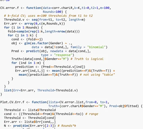
Predictive Models with Built-in Cross-Validation

At this point of the work, there is enough information to start developing predictive models with

brain relationships coming from functional connectivity. This process will involve three steps:

(20)

The first subject characteristic selected as the response variable was Gender, which happens to

have three categories. The input variables will be given by the averaged correlations within each

subject. There is going to be as many predictor as region combination selected for the model.

Because correlations cannot be summed, the following expression was used to summarized the

features values.

𝑌 = 𝑠𝑞𝑟𝑡(𝑚𝑒𝑎𝑛(𝑐𝑜𝑟𝑟𝑠

2

))

The three categories corresponding to the response variable are:



Male



Female



Undefined

#Gender Categories

## [1] "M" "F" "U"

Because the response is a categorical variable, the problem leans to be a classification type. The

error percentages previously calculated will serve as reference to include meaningful features in

the model. Since all error percentages were ordered from lowest to highest, every sample taken

from this dataset, ensure the best predictors. The set of ranked features for each model will be

selected by the following criteria:



Case 1: The first set of predictors, that will be selected, correspond to the set of correlations

where the variability coming from the error was lower than the first quartile of the

distribution.

o

Results: 1666 predictors

14

– Random Forest.



Case 2: The second set of predictors will be given by the set of correlations where the

variability coming from the error is the minimum value of the distribution.

o

Results: 1 predictor – Logistic Regression – The Best Predictor



Case 3: The third set of predictors will be given by the set of correlations supported by the

statistical technique used to model the data without causing complete or quasi-separation.

(21)

The supported set with less predictors of all statistical technique will be replicated over the

rest for comparison purposes.

o

Logistic Regression AIC: 120 predictors

o

Logistic Regression Best Predictors: 120 predictors

o

Linear Discriminant Analysis: 120 predictors

o

Random Forest: 120 predictor

Finally, the “Undefined” category of the response variable will be excluded from the analysis,

because only contains one subject of the 820, which makes it irrelevant.

Ranked Predictors and Model Assumptions

The following output present a sample of the dataset containing all region combinations with their

error percentages. These results are already ranked for the best error percentages

15

.

head(bestCombs.df,12) ## [,1] [,2] [,3] ## [1,] 27.47 11 61 ## [2,] 31.78 13 61 ## [3,] 32.36 12 14 ## [4,] 32.64 11 62 ## [5,] 33.24 11 13 ## [6,] 33.35 8 66 ## [7,] 34.14 7 61 ## [8,] 34.50 65 67 ## [9,] 34.55 62 65 ## [10,] 34.66 12 62 ## [11,] 34.86 12 66 ## [12,] 35.29 65 66

The first column correspond to the calculated error percentage, the second column is the first

region and the third column is the second region of the combination. Based on that sample, it was

possible to obtain the following set:

## Group.1 x Gender Age ## 1 100206 0.4417249 M 26-30 ## 2 100307 0.3409603 F 26-30 ## 3 100408 0.6088309 M 31-35 ## 4 100610 0.4345944 M 26-30 ## 5 101006 0.3359919 F 31-35 ## 6 101107 0.6758970 M 22-25

(22)

## 7 101309 0.4469654 M 26-30 ## 8 101915 0.4621885 F 31-35 ## 9 102008 0.5967210 M 22-25 ## 10 102311 0.5345915 F 26-30 ## 11 102513 0.4547970 M 26-30 ## 12 102816 0.4242340 F 26-30

Now let’s take a look to the assumptions of the new dataset (n < Q1) and the original dataset.

Both dataset samples seems to approximate the normal distribution. The main difference between

(23)

a more centered distribution, the sample dataset is skewed to the left. As expected, the filtered data

is centered towards higher correlation values, because of the lower error percentages.

Model 1: Logistic Regression with the Best Predictor - Gender

Now let’s see, how the simplest model with intercept, can predict subject’s gender based on the

relationship between the brain region combination with the lowest error percentage using logistic

regression.

## ## Call:

## glm(formula = as.factor(Gender) ~ corrsLowest, family = binomial(link = "l ogit"),

## data = corr.charLowest) ##

## Deviance Residuals:

## Min 1Q Median 3Q Max ## -1.7999 -1.0277 -0.5818 1.0742 2.2592 ##

## Coefficients:

## Estimate Std. Error z value Pr(>|z|) ## (Intercept) -3.7360 0.3839 -9.731 <2e-16 *** ## corrsLowest 6.2796 0.6623 9.481 <2e-16 *** ## ---

## Signif. codes: 0 '***' 0.001 '**' 0.01 '*' 0.05 '.' 0.1 ' ' 1 ##

## (Dispersion parameter for binomial family taken to be 1) ##

## Null deviance: 1125.7 on 818 degrees of freedom ## Residual deviance: 1015.7 on 817 degrees of freedom

## AIC: 1019.7

##

## Number of Fisher Scoring iterations: 3

The generated model shows p-values lower than 0.05, which indicates statistical significance of

the predictor. The following results correspond to the predictions calculated using the model for

the 819 subjects.

## CorrHatFac ## F M Sum ## F 274 180 454 ## M 111 254 365 ## Sum 385 434 819

#Accuracy Percentage

(24)

The model with one predictor and the intercept was capable of successfully classified 274 females

as females, and 254 males as males. On the other side, it incorrectly classified 111 females as

males, and 180 males as females. Based on these results, the model performed predictions with a

64.47 percent of accuracy. The following step consist on using a model selection procedure to

determine which predictors are more relevant for the next sample of the analysis.

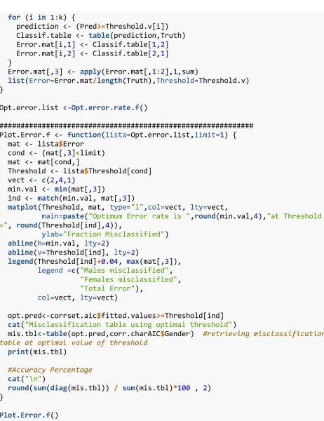
The following output compares misclassification tables using optimal thresholds with and without

cross-validation.

## The optimal threshold for the 10-fold cross validation is: 0.5454545454545 46

## gender.prediction F M ## FALSE 364 187 ## TRUE 90 178 ## [1] 66.18%

## The error rate for 10-fold cv is:0.338217338217338

The model with cross validation got an accuracy rate of 66.18 percent, while the

non-cross-validated model with optimal threshold had a 66.67 percent.

Model 2: Logistic Regression with AIC Selection - Gender

#Showing a summary of the results

## ## Call:

(25)

## V18 + V115 + V64 + V34 + V20 + V5 + V40 + V108 + V31 + V3 +

## V99 + V51 + V113 + V82 + V83 + V95, family = binomial(link = "logit"), ## data = corr.charAIC)

##

## Min 1Q Median 3Q Max ## -3.1475 -0.4474 -0.0482 0.4524 2.6914 ##

## Coefficients:

(26)

## V95 -2.5757 1.1182 -2.303 0.021259 * ## ---

## Signif. codes: 0 '***' 0.001 '**' 0.01 '*' 0.05 '.' 0.1 ' ' 1 ##

## AIC: 616.79

##

## Number of Fisher Scoring iterations: 6

#Contingency table and marginal sums

cTab.AIC <- table(corrset.aic$data$Gender, CorrHatFac.AIC)

addmargins(cTab.AIC) ## CorrHatFac.AIC ## F M Sum ## F 384 70 454 ## M 47 318 365 ## Sum 431 388 819

#Accuracy Percentage

round(sum(diag(cTab.AIC)) / sum(cTab.AIC)*100 , 2) ## [1] 85.71%

After the selection procedure, the resulting model possess 40 predictors, where 34 of those have

p-values lower than 0.05, expressing statistical significance. Comparing AIC values

16

, the model

with just one predictor has a higher value of 1019.7 versus the last model with 616.79, which

express better evidence towards this model. The AIC model was capable of successfully classified

384 females as females, and 318 males as males. On the other side, it incorrectly classified 47

females as males, and 70 males as females. Based on these results, the model performed predictions

with an 85.71 percent of accuracy. Now is time to validate how the model will perform in practice

using 10-fold cross-validation.

(27)

cross-validation.

## Misclassification table using optimal threshold ## opt.pred F M

## FALSE 395 54 ## TRUE 59 311 ## [1] 86.20%

There is not much difference coming from the error rates. While the model without

validation and optimal threshold was able to predict with an accuracy rate of 86.20%, the

cross-validated model got an 85.59% accuracy rate. All three models had similar performance for the

AIC selected predictors.

Model 3: Logistic Regression with Ranked Predictors - Gender

## Call:

## glm(formula = as.factor(Gender) ~ ., family = binomial(link = "logit"), ## data = corr.charLR)

##

(28)

## Coefficients:

(29)

(30)

## V98 3.25078 2.26334 1.436 0.150924 ## V99 4.37004 3.71561 1.176 0.239543 ## V100 -2.95125 2.95542 -0.999 0.317994 ## V101 -1.97238 3.83430 -0.514 0.606969 ## V102 5.38394 3.32042 1.621 0.104918 ## V103 -0.34987 1.96531 -0.178 0.858706 ## V104 0.38002 2.96253 0.128 0.897932 ## V105 -1.55366 2.16217 -0.719 0.472408 ## V106 6.78504 7.60361 0.892 0.372208 ## V107 -2.15777 4.90537 -0.440 0.660025 ## V108 3.37098 1.60759 2.097 0.036001 * ## V109 4.38324 2.41808 1.813 0.069879 . ## V110 -2.03526 2.57050 -0.792 0.428490 ## V111 5.44921 6.99906 0.779 0.436238 ## V112 -3.43345 2.61566 -1.313 0.189302 ## V113 -3.19998 3.33536 -0.959 0.337353 ## V114 -3.02525 1.79012 -1.690 0.091034 . ## V115 -4.99377 2.54012 -1.966 0.049303 * ## V116 -9.96946 2.82168 -3.533 0.000411 *** ## V117 -0.87289 3.14468 -0.278 0.781338 ## V118 7.22483 3.53859 2.042 0.041179 * ## V119 6.80636 2.83647 2.400 0.016413 * ## V120 -5.27296 3.10517 -1.698 0.089484 . ## ---

## Signif. codes: 0 '***' 0.001 '**' 0.01 '*' 0.05 '.' 0.1 ' ' 1 ##

## AIC: 699.53

##

## Number of Fisher Scoring iterations: 7 ## CorrHatFac.LR

## F M Sum ## F 398 56 454 ## M 44 321 365 ## Sum 442 377 819 ## [1] 87.79%

The model obtained using logistic regression contains 29 variables with p-values lower than

0.05for statistical significance, intercept included. While the AIC value is lower than the one

predictor model, the AIC is higher than the AIC selected predictors. . Based on these results, the

model performed predictions with an 85.71 percent of accuracy. Now is time to validate how the

(31)

cross-validation.

## Misclassification table using optimal threshold ## opt.pred F M

## FALSE 417 56 ## TRUE 37 309 ## [1] 88.64%

There is not much difference coming the accuracy of the models above. While the model without

cross-validation and optimal threshold was able to predict with an accuracy rate of 88.64%, the

cross-validated model got an 87.67% accuracy rate. All three models had similar performance for

(32)

Model 4: Linear Discriminant Analysis with Predictors - Gender

The second statistical technique proposed for this classification problem was Linear Discriminant

Analysis. This method allows characterizing two or more classes of objects based on means and

variances, whose results must be used as a linear classifier.

## Length Class Mode ## prior 2 -none- numeric ## counts 2 -none- numeric ## means 240 -none- numeric ## scaling 120 -none- numeric ## lev 2 -none- character ## svd 1 -none- numeric ## N 1 -none- numeric ## call 3 -none- call ## terms 3 terms call ## xlevels 0 -none- list ## Actual

## Predicted F M ## F 402 44 ## M 52 321 ## [1] 88.28%

The LDA model was capable of successfully classified 402 females as females, and 321 males as

males. On the other side, it incorrectly classified 52 females as males, and 44 males as females.

Based on these results, the model performed predictions with an 88.28 percent of accuracy. Now

(33)

cross-validation.

Classif.table ##

## F M ## F 402 44 ## M 52 321 ## [1] 88.28%

# Misclassification error of the 100 rounds of 10 fold CV

CV.error <- CV.error.f.1()

## Average misclassified cases using 10 fold CV = 171.63

## Standard error of total minimized error of misclassification = 0.5054561 ## F M

## F 294 257 ## M 160 108 ## [1] 49.08%

The LDA technique is presenting a different behavior compared to the other techniques. The

accuracy rate for the trained model and the best prior is almost the same. On the other hand, the

cross-validated model using best prior, is presenting a lower accuracy rate of 49.08%.

Model 5: Random Forest with Ranked Predictors - Gender

The last statistical technique to be applied in this classification problem will be Random Forest.

This is a more general technique that uses a multitude of decision trees to determine which class

is the best for the object to be classified.

## Random Forest ##

## 819 samples ## 120 predictors

## 2 classes: 'F', 'M' ##

## No pre-processing

## Resampling: Cross-Validated (10 fold, repeated 3 times) ## Summary of sample sizes: 738, 737, 736, 738, 738, 737, ... ## Resampling results:

##

(34)

##

## Tuning parameter 'mtry' was held constant at a value of 11

The accuracy rate corresponding to the random forest technique when using 120 ranked predictors

with mtry

17

constant is 72.80 percent.

## Random Forest ##

## 2 classes: 'F', 'M' ##

## Resampling: Cross-Validated (10 fold, repeated 3 times) ## Summary of sample sizes: 737, 736, 737, 736, 738, 737, ... ## Resampling results across tuning parameters:

##

## mtry Accuracy Kappa ## 4 0.7245164 0.4355670 ## 7 0.7224595 0.4316812 ## 9 0.7253294 0.4371518 ## 25 0.7285918 0.4437038

(35)

## 50 0.7245267 0.4358481 ## 57 0.7236387 0.4346460 ## 60 0.7265290 0.4403687 ## 68 0.7302224 0.4479660 ## 73 0.7228603 0.4335629 ## 94 0.7265786 0.4410374 ## 98 0.7265691 0.4410037 ## 105 0.7286017 0.4453208 ## 113 0.7269409 0.4412480 ## 118 0.7277939 0.4432234 ##

## Accuracy was used to select the optimal model using the largest value. ## The final value used for the model was mtry = 68.

Using a dynamic value for mtry, its shows that the best configuration for this set of ranked

predictors correspond to best 68, where the accuracy rate ends up at 73.02 percent.

Model 6: Regression with Ranked Predictors - Age

The second subject characteristic selected as the response variable was Age, which happens to

have a five ordinal type categorical variable. Because the first statistical technique to apply will be

(36)

corr.charRE$AgeCod[corr.charRE$Age == "22-25"] <- 23.5

corr.charRE$AgeCod[corr.charRE$Age == "26-30"] <- 28

corr.charRE$AgeCod[corr.charRE$Age == "31-35"] <- 33

corr.charRE$AgeCod[corr.charRE$Age == "36+"] <- 36

Similar to the previous models, the regression analysis will be performed using the ranked

predictors, thus the model accuracy could be compare with the others at the same level. Now the

summary of the model is presented.

## Call:

## lm(formula = AgeCod ~ ., data = corr.charRE) ##

## Residuals:

## Min 1Q Median 3Q Max ## -8.8707 -2.2918 0.0086 2.4354 8.3629 ##

## Coefficients:

(37)

(38)

## V81 3.128931 2.951677 1.060 0.28949 ## V82 -0.267533 2.819736 -0.095 0.92444 ## V83 0.130288 2.666107 0.049 0.96104 ## V84 -5.856971 1.938523 -3.021 0.00261 ** ## V85 4.589318 4.224905 1.086 0.27774 ## V86 2.951686 2.240163 1.318 0.18806 ## V87 -6.669455 4.239618 -1.573 0.11614 ## V88 1.842232 1.982811 0.929 0.35316 ## V89 0.290086 2.070916 0.140 0.88864 ## V90 -3.633582 2.702141 -1.345 0.17916 ## V91 -0.173392 2.381239 -0.073 0.94197 ## V92 3.731865 6.275424 0.595 0.55225 ## V93 0.009575 1.970768 0.005 0.99612 ## V94 -1.840717 2.820104 -0.653 0.51416 ## V95 -3.190036 2.095833 -1.522 0.12844 ## V96 -0.463682 2.273817 -0.204 0.83847 ## V97 0.440872 4.282425 0.103 0.91803 ## V98 0.837597 2.000288 0.419 0.67554 ## V99 -0.080477 3.069807 -0.026 0.97909 ## V100 -2.988035 2.448997 -1.220 0.22284 ## V101 2.035410 3.413008 0.596 0.55112 ## V102 4.335541 2.597115 1.669 0.09549 . ## V103 -0.935374 1.662980 -0.562 0.57398 ## V104 0.961077 2.571799 0.374 0.70874 ## V105 -0.346836 1.901066 -0.182 0.85529 ## V106 -0.749740 6.669970 -0.112 0.91053 ## V107 -3.070646 4.081667 -0.752 0.45212 ## V108 -4.344954 1.488466 -2.919 0.00362 ** ## V109 -0.735741 2.050528 -0.359 0.71985 ## V110 -1.248119 2.214298 -0.564 0.57316 ## V111 5.140838 5.777060 0.890 0.37384 ## V112 0.109820 2.159888 0.051 0.95946 ## V113 -1.605397 2.860955 -0.561 0.57488 ## V114 -0.223579 1.566308 -0.143 0.88653 ## V115 4.346832 2.268017 1.917 0.05570 . ## V116 5.241648 2.332630 2.247 0.02494 * ## V117 0.650741 2.617017 0.249 0.80370 ## V118 -0.825011 3.060201 -0.270 0.78755 ## V119 -0.431792 2.363876 -0.183 0.85512 ## V120 0.954559 2.666351 0.358 0.72045 ## ---

## Signif. codes: 0 '***' 0.001 '**' 0.01 '*' 0.05 '.' 0.1 ' ' 1 ##

## Residual standard error: 3.279 on 699 degrees of freedom ## Multiple R-squared: 0.2881, Adjusted R-squared: 0.1658 ## F-statistic: 2.357 on 120 and 699 DF, p-value: 5.935e-12 ## actuals predicteds

(39)

mape <- mean(abs((RealPredsRE$predicteds - RealPredsRE$actuals))/RealPredsRE$

actuals) mape*100

## [1] 9.093%

The model obtained using regression analysis contains 12 variables with p-values lower than

0.05for statistical significance, intercept included. While the r-squared has a value of 0.2881, the

adjusted r-squared has a lower value of 0.1658. Based on these results, the model performed

predictions with a 9.1 percent of accuracy. Now is time to validate how the model will perform in

practice using 10-fold cross-validation.

## Linear Regression ##

## 820 samples ## 120 predictors ##

##

## RMSE Rsquared MAE ## 3.574496 0.09225774 2.960404 ##

## Tuning parameter 'intercept' was held constant at a value of TRUE

After cross-validate the regression model, there is not much difference in terms of the behavior of

the model. The r-square measure is for both, the cross-validated and the no cross-validated is

around 9 percent.

Model 7: Random Forest with Ranked Predictors – Age

Maintaining the response variable as continuous is possible apply Random Forest to the same set of

ranked predictor and evaluate the performance improvement.

## Random Forest ##

## 820 samples ## 120 predictors ##

(40)

## Resampling results: ##

## RMSE Rsquared MAE ## 3.432033 0.0975931 2.842126 ##

The Random Forest with constant mtry got similar results to the previous model. The r-squared

value is also close to 9 percent.

Model 8: Random Forest with Ranked Predictors – Age as Categorical

Initially the ordinal response variable was transformed to numerical type as a way to avoid losing

order information. This process was done taking the mid-point of the range of every category.

Because the model did not perform well, the same statistical technique will be apply over the same

set of values but using a classification perspective. Random Forest allows to perform models for

both, prediction and classification cases. The first configuration will be maintaining mtry constant

over the whole procedure.

## Random Forest ##

## 4 classes: '23.5', '28', '33', '36' ##

##

## Accuracy Kappa ## 0.4699289 0.1235139 ##

The model was able to classified categories with an accuracy of 47 percent. Now lets see if there

is a change coming of setting mtry dynamic.

## Random Forest ##

## 4 classes: '23.5', '28', '33', '36' ##

(41)

## Summary of sample sizes: 737, 739, 737, 737, 737, 739, ... ## Resampling results across tuning parameters:

##

## mtry Accuracy Kappa ## 1 0.4573678 0.09110569 ## 6 0.4739267 0.12944764 ## 21 0.4712190 0.12935359 ## 23 0.4784931 0.14028927 ## 24 0.4781756 0.14082136 ## 35 0.4735987 0.13380489 ## 41 0.4629691 0.11774828 ## 45 0.4752790 0.13937075 ## 54 0.4679813 0.12664317 ## 66 0.4688200 0.13006895 ## 80 0.4715458 0.13493838 ## 82 0.4683036 0.12999767 ## 106 0.4764338 0.14336838 ## 113 0.4804694 0.15063575 ##

## Accuracy was used to select the optimal model using the largest value. ## The final value used for the model was mtry = 113.

Configuring mtry value as dynamic, its shows that the best configuration for this set of ranked

(42)

Accuracy Assessment and Recommendations

Having applied four different statistical methods

18

to classify/predict two relevant subject’s traits,

is possible to make assessments on how these models performed based on the accuracy rate

obtained with each method. For contrast purposes, all models were performed using the same set

of ranked predictors, which makes possible to determine the best choice using similar amount of

computational resources. The following table shows a summary of the accuracy measurement for

each technique at every level of optimization.

Model Configuration

Accuracy

Predictor

s

Respons e

Statistical

Technique Details

AIC/R-Sq

Standar d

Optimal/Mt

ry CV

BesttPre d

1 Gender

Logistic Regression

Best Predictor

1019.7

0 64.47 66.67 66.1

8 Females

120 Gender

AIC Logistic Regression Ranked Predictor s (40 Pred.

left) 616.79 85.71 86.20 85.5

9 Males

120 Gender

Logistic Regression

Ranked Predictor

s 699.53 87.79 88.64

87.6

7 Females

120 Gender

Linear Discrimina nt

Ranked Predictor

s NA 88.28 88.28

49.0

8 Females

120 Gender

Random Forest Both cross-validated - Mtry dynamic vs Mtry

constant NA NA 73.02

72.8

0 Females

120 Age Regression 9.10 NA NA NA NA

120 Age

Random Forest

Mtry

constant 9.75 NA NA NA NA

120 Age

Random Forest

Mtry constant vs Mtry

dynamic NA NA 48.40

46.9

9 Females

(43)

Both prediction and classification analysis will get a different accuracy measurement at each level

of the process. The standard level correspond to the training of the model using the entire dataset

and using the same values to predict. The second level corresponds to the same standard process

but adding an optimization technique to determine the best threshold. The last level represent a

cross-validation procedure utilizing the optimal threshold.

The motivation of using cross-validation falls in the fact that when a model is fitted, it usually fit

the same training dataset. Without cross-validation, the accuracy measure only tells how the model

perform in that specific dataset. The main interest in this case is having an accuracy measure that

could represent the correctness of the model for any new dataset of this type. For this reason, the

goodness of the model only will be evaluated based on cross-validated results.

The first interesting thing to point out is how good the procedure used to select the best features

was. The model with only one predictor and the intercept was capable of predicting accurately

66% of the cases. It should be noted that every feature to be included will be worse than the

previous one when they follow the ranked order. This means that at some point adding more

features will not be significant for the increment of the accuracy rate.

Selecting 120 ranked predictors to perform each statistical technique, was the optimal point

between getting an adequate accuracy rate, manage viable computational times and avoiding

irrelevant predictors. The following output represent the top 6 best predictors.

head(bestCombs.df) ## [,1] [,2] [,3] ## [1,] 27.47 11 61 ## [2,] 31.78 13 61 ## [3,] 32.36 12 14 ## [4,] 32.64 11 62 ## [5,] 33.24 11 13 ## [6,] 33.35 8 66

Looking closely at the top six best region combination, it is noticeable that these low error regions

share the same side of brain hemisphere. For example,

Frontal_Inf

and

Parietal_Inf

are in the left

hemisphere, while

Frontal_Mid

and

Angular

are in the right side.

1. Precentral_L 16. Frontal_Inf_Orb_R31. Cingulum_Ant_L46. Cuneus_R61. Parietal_Inf_L 2. Precentral_R 17. Rolandic_Oper_L32. Cingulum_Ant_R47. Lingual_L62. Parietal_Inf_R 3. Frontal_Sup_L 18. Rolandic_Oper_R33. Cingulum_Mid_L48. Lingual_R63. SupraMarginal_L 4. Frontal_Sup_R 19. Supp_Motor_Area_L34. Cingulum_Mid_R49. Occipital_Sup_L64. SupraMarginal_R 5. Frontal_Sup_Orb_L 20. Supp_Motor_Area_R35. Cingulum_Post_L50. Occipital_Sup_R65. Angular_L 6. Frontal_Sup_Orb_R 21. Olfactory_L36. Cingulum_Post_R51. Occipital_Mid_L66. Angular_R 7. Frontal_Mid_L 22. Olfactory_R37. Hippocampus_L52. Occipital_Mid_R67. Precuneus_L 8. Frontal_Mid_R 23. Frontal_Sup_Medial_L38. Hippocampus_R53. Occipital_Inf_L68. Precuneus_R 9. Frontal_Mid_Orb_L 24. Frontal_Sup_Medial_R39. ParaHippocampal_L54. Occipital_Inf_R69. Paracentral_Lobule_L 10. Frontal_Mid_Orb_R 25. Frontal_Med_Orb_L40. ParaHippocampal_R55. Fusiform_L70. Paracentral_Lobule_R 11. Frontal_Inf_Oper_L 26. Frontal_Med_Orb_R41. Amygdala_L56. Fusiform_R71. Caudate_L

(44)

Evaluating the models, Linear discriminant technique had a good performance using the optimal

prior, but it fell down in the cross-validation procedure going from 88.28 to 49.08 percent accuracy

rate. For this reason, this was the first discarded technique of the three used to model gender.

Random Forest also performed well using mtry set constant and little bit better when the parameter

was dynamic. It went from 72.80 to 73.02 percent accuracy rate. It was the most robust technique,

allowing to model gender using over a thousand predictors. The results with more than 200

predictors were not included because they did not affected much the accuracy rate

19

. Although the

Random Forest model had a good performance and the best robustness, it was discarded because

the last two model outperformed its results.

The statistical technique propose by this investigation, which is the best adequate to classify the

subject gender based on functional connectivity, correspond to Logistic Regression. The AIC

Logistic Regression model was capable of getting an 85.6 percent accuracy rate. Alternatively, the

Logistic Regression model maintaining the entire set of ranked predictor was capable of getting

an 87.7 percent accuracy rate. Is interesting to point out that the model with the AIC features was

better classifying males, whereas the complete ranked model was better classifying females.

Even though the Logistic Regression technique was not as robust as the Random Forest, it was

able to get better accuracy rates after cross-validation. Moreover, because this type of model is

based purely on linear relationships, is easier to explain and be implemented by other researchers

with low or no expertise in statistical analysis.

Speaking of Age as the second response variable, the first technique, corresponding to Regression

analysis, failed trying to capture the pattern to predict the subject’s age. This variable was given

as an ordinal type level of measurement. The first approach consisted on converting each category

to continuous and avoid losing information coming from the order. In the same way, Random

Forest were performed using the same specification and also failed, getting an r-squared of 9.75

and 9.10 for the Regression technique.

The results changed for good when the variable was treated as a nominal type with five categories.

The Random Forest technique using mtry dynamic was capable of getting 48.80 percent accuracy

rate. Any set of predictors between 200 and 1600 where presenting similar rates of accuracy.

(45)

Bibliographic Reference

Vul E, Harris C, Winkielman P, Pashler H. Puzzlingly high correlations in fMRI studies of

emotion, personality, and social cognition. Perspect. Psychol. Sci. 2009.

Finn ES, et al. Functional connectome fingerprinting: identifying individuals using patterns of

brain connectivity. Nat Neurosci. 2015.

Van Essen DC, et al. The WU-Minn human connectome project: an overview. Neuroimage. 2013.

Gabrieli JD, Ghosh SS, Whitfield-Gabrieli S. Prediction as a humanitarian and pragmatic

(46)

Appendix

(47)

Feature Selection Procedure

Best Region Combination

(48)

R Code

Reading in Data and Loading Packages

###################################### Reading Data ######################### #################

#Loading Packages

library(memisc)#Reordering features

library(lme4)#Fitting linear mixed-effects model

library(nortest)#Testing normality

library(MASS)#Linear Discriminant Analysis

library(randomForest)#RF Decision trees

library(DAAG)# k-fold CV for continuos

library(caret)#k-fold CV linear regression

library(e1071)

#Reading in the Data

#Setting Working Directory

thesisPath<-"D:\\GuenadieNibbs\\Classes\\AppliedStatisticsMS\\Thesis\\Data\\"

setwd(thesisPath)

getwd()

#Loading Brain Activity data from file#

load("Scans.arr") #27.87 seg elapsed #Array dimensions (Whole dataset)

dim(Scans.arr)

#Printing subset to show array structure (5 Nodes, 3 Regions, 2 Scans, 2 Subj ects)

Scans.arr[1:5,1:3,1:2,1:2]

#Reordering array by subject's ID

Scans.arr<-reorder(Scans.arr,dim=4, indices = 1:820) #4.19 seg elapsed #Loading Subjects characteristics

characteristics.df<-read.csv("BrainsubjectsCopy.csv", header = T, stringsAsFa ctors = F)

dim(characteristics.df)

sample(characteristics.df,10)

Exploratory:

Data Sampling Parameters

###################################### DataSet Breakdown #################### ##################

#Creating a function to calculate correlations on pre-specified number of reg ions.

(49)

#Brain Activity -> min=1 max=1200

inibac<-1

endbac<-1200

bac<-c(inibac:endbac)

#Regions -> min=1 max=116

iniReg<-1

endreg<-116

#regions<-c(1,2) -> To gather not sequential regions.

regions<-c(iniReg:endreg)

#MRIs -> min=1 max=4

inimri<-1

endmri<-4

mris<-c(inimri:endmri)

#Patients -> min=1 max=820

inipat<-1

endpat<-820

patiens<-c(inipat:endpat)

#Lengths#

bl<-length(bac) rl<-length(regions) ml<-length(mris) pl<-length(patiens)

exp.reg<-(((rl*(rl+1))/2)-rl)#Amount of corrs within 1 scan

exp.scan<-(((rl*(rl+1))/2)-rl)*ml #Amount of corrs within ml scans (max. 4) a nd 1 subject

exp.pat<-(((rl*(rl+1))/2)-rl)*ml*pl #Total amount of correlations within pls (max. 820)

Features Selection:

Variance Components.

###################################### Variance Components ################## #######################

#Correlation Function with VC features (2 columns output: corr|Sub)

corr.fun.Esp<-function(a,b,c,d){ scans.subset<-Scans.arr[a,b,c,d]

corr.arr<-apply(scans.subset,c(3,4), cor)

corr.vect<-as.vector(corr.arr[corr.arr[1:(2^2)]!=1,,])#Reg fixed at 2 becau se they enter 2 at a time always.

corr.mat<-as.matrix(unique(corr.vect)) pat.sec<-rep(1:pl, each=4)# Fixed to 4

corr.mat<-do.call(cbind,list(corr.mat,pat.sec,deparse.level = 0)) return (corr.mat)

}

#Creating dataframe to host all region combinations C(116,2)

(50)

f Regions

regComb<-unique(t(apply(regComb, 1, sort)))#Removing duplicates pairs

regComb<-regComb[regComb[,1]!=regComb[,2], , drop = F]#Removing X=Y

varComp.mat<-matrix(NA,nrow(regComb),1)#Creating empty matrix to be loaded

nrow(varComp.mat) == (((rl*(rl+1))/2)-rl)

#Calculating all variance component for the specified subset of regions #2244 .85 seg (37.4 min) elapsed

for(i in 1:nrow(regComb)){

regs<-c(regComb[i,1],regComb[i,2])#Getting two regions at a time

corrs<-corr.fun.Esp(bac,regs,mris,patiens)#Getting correlations for 1 combi nation (3280)

study.mod<-lmer(corrs[,1] ~ (1|corrs[,2]), data = as.data.frame(corrs)) #Ra ndom Effects Model

var.comp<-as.data.frame(VarCorr(study.mod),deparse.level = 0)[,c(1,4)] error.perct<-round((var.comp[2,2]/sum(var.comp[,2]))*100,2)

varComp.mat[i,]<-error.perct }

#Creating Error Percentage Matrix

errorPerct.mat<-matrix(NA,rl,rl)#Empty Matrix #Feeling the matrix in the right order

n=1

for(i in 1:rl){

for(j in 1:rl){ if (i==j) {

errorPerct.mat[i,j]<-NA

} else if (j<i){ #Nothing

} else {

errorPerct.mat[i,j]<-varComp.mat[n,1] errorPerct.mat[j,i]<-varComp.mat[n,1] n=n+1

}}}

class(errorPerct.mat) <- "numeric" #Changin to numeric

errorPerct.mat[is.na(errorPerct.mat)]<-100 #Changing NAs with 100

errorPerct.mat[1:5,1:5] #Matrix Preview #Plotting variability(Error%) Matrix

par(mar=c(1,1,1,1))

image(errorPerct.mat)

Criteria - Selection Cases.

(51)

bestCombs.df<-cbind(varComp.mat,regComb)#Matching Error% with its region comb ination

bestCombs.df<-bestCombs.df[order(bestCombs.df[,1]),]

dim(bestCombs.df)

head(bestCombs.df)

#Extracting lows t Error% reg combinations - Q1 and MIN as reference #Getting Q1 and MIN

fiveMeasures<-summary(varComp.mat)

Q1<-as.numeric(sub('.*:', '', fiveMeasures[2]))# First quartile

min<-as.numeric(sub('.*:', '', fiveMeasures[1]))# Minimun value

########################################################### Case 1 - Lowest E rror% (Min)

bestCombsMin.df<-subset(bestCombs.df,bestCombs.df[,1] == min)

head(bestCombsMin.df)

regCombLowest<-bestCombsMin.df[,2:3,drop = FALSE]

dim(regCombLowest)

#Calculating correlations for the lowest Error%

corrsMin<-matrix(NA,1,2)#Creating a matrix to be filled

for(i in 1