Queuing disciplines on Linux made easy

Implementation of AQMs on Linux made Easy

Stephen Braithwaite

Department of Mathematics and Computing

The University of Southern Queensland, Toowoomba, QLD

Abstract

This is a project to implement a Mice and Elephants queueing discipline, which favours short flows over long flows, on Linux. The project has three aims. The first aim is to produce a prototype Mice and Elephants router for the purpose of further evaluation of the Mice and Elephants strategy and the Shortest Job First strategy. The second aim is to make a contribution to Linux by making my implementation as code that is both fit for distribution with Linux and useful in a small business or domestic setting. The third aim is to explore and document a method of creating Linux queueing disciplines in general.

Contents

1 Introduction 9

1.1 Rationale . . . 10

1.2 Mice and Elephants strategies . . . 10

1.3 Linux Queueing Disciplines . . . 11

1.4 Ingress Filter . . . 11

1.5 Documentation Created . . . 12

1.6 User Space Development Environment . . . 12

1.7 Overview . . . 12

2 Active Queue Management 15 2.1 Random Early Detection . . . 16

2.2 Fairness algorithms . . . 19

2.3 Mice and Elephants . . . 20

2.4 A Mice and Elephants Queueing Discipline . . . 21

2.5 A Mice and Elephants Ingress Filter . . . 22

3 Linux Queueing Disciplines 27 3.1 History of Net-4 . . . 27

3.2 Linux Networking Concepts - Classifiers, Policers, Queueing Disciplines and Filters . . . 27

3.2.1 U32 . . . 30

3.2.2 HTB . . . 30

3.3 Kernel Modules . . . 31

3.4 The Linux Queueing Discipline Interface . . . 31

3.5 Setting up a Linux Queueing Discipline Interface . . . 31

4 Implementation 33 4.1 Summary of Queueing Disciplines Developed . . . 33

4.1.1 Drop Tail . . . 33

4.1.2 RED . . . 33

4.1.3 ARED . . . 34

6 CONTENTS

4.1.4 Mice and Elephants . . . 35

4.1.5 Mice and Elephants Classifier . . . 36

4.2 Design Details . . . 37

4.2.1 RED . . . 37

4.2.2 ARED . . . 39

4.2.3 Mered - The First Mice and Elephants Queueing Discipline . . . 39

4.2.4 Meredt - The Second Mice and Elephants Queueing Discipline . . 44

4.2.5 Meredtf - The Mice and Elephants Ingress Filter . . . 48

4.3 Queueing Discipline Development Environments . . . 49

4.3.1 Tcsim . . . 49

4.3.2 User Mode Linux . . . 50

4.3.3 Umlsim . . . 51

4.3.4 Linquede . . . 52

4.3.5 Comparison of AQM testing environments . . . 52

4.4 Platform . . . 53

5 Testing 55 5.1 Load Testing . . . 55

5.2 Test Harness . . . 56

5.3 Three Experimental Scenarios . . . 56

5.3.1 TheMice OnlyScenario . . . 57

5.3.2 TheCongestedScenario . . . 57

5.3.3 TheMice and ElephantsScenario . . . 57

5.3.4 Results . . . 57

6 Deployment and Configuration 59 6.1 Congestion on the Edge Router . . . 59

6.2 Dropping Packets at the Gateway Router . . . 59

6.3 Edge Router Buffer Level Estimation . . . 61

6.4 Testing the Idea . . . 63

7 Conclusion 65

A Linquede HOWTO 75

B Qdisc Man Page 93

C ARED Man Page 99

D MERED Man Page 105

CONTENTS 7

F MEREDTF Man Page 117

Chapter 1

Introduction

Within IP networks, packets may arrive at a router faster than they may be placed onto the network. When this happens, they are stored in a queue. This queue may not be a pure queue or FIFO, however, in the sense that the first packet that arrived will not nec-essarily be placed onto the network first. In order to improve performance, the algorithm managing this queue may choose to deliver packets in a different order to that in which they arrived. It may also choose to drop packets or slightly modify (mark) them. Such strategies or algorithms for choosing what packets to drop or mark and what order to de-liver them in are called queuing disciplines. A non trivial queuing discipline, one that implements more than pure queueing is called anactive queue management(AQM) [44].

In this project I have investigated and implemented a particular type of AQM, called a mice and elephantsAQM [31]. A mice and elephants AQM can improve the responsive-ness of communication. In the context of a mice and elephants queueing discipline, the shorter flows are calledmice, and the longer flows are calledelephants[45]. A mice and elephants queuing discipline works by giving priority to the mice.

The queuing disciplines that I have implemented are suitable for use in the access net-work for a business or domestic residence. I have implemented them in the Linux operat-ing system, due to the ready availability of the source code and the software development tools. On Linux, the code module that implements a queueing discipline algorithm is also called aqueueing discipline[21].

As part of this project, the mice and elephant AQM has been implemented in the form of Linux queuing disciplines. These have documented in the form of Linuxman pages. An environment for the development of queuing disciplines on Linux has also been created. This has been documented in the form of a HOWTO.

10 CHAPTER 1. INTRODUCTION

1.1

Rationale

Responsiveness is one of the key qualities of an internet service. People will judge an internet service by how long it takes to have keystroke echoed, or to see a web page.

During periods of high congestion, the long flows although few in number, account for a disproportionate amount of the traffic flow [45]. The remaining traffic is made up of short flows. Thus, the long flows are termed elephantsand the short flows are termed mice.

Long flows, such as a large download of software, are typically not sensitive to the delays caused by this congestion, but the short flows are [75]. You can imagine that if packets generated by keystrokes in a telnet session had to wait in a queue congested by packets from a large download, the telnet session will be adversely affected by the delays. Fair queueing is one way to improve the responsiveness of the internet. By ensuring ”fair” use amongst traffic flows, we can prevent heavy flows from making the internet unusable for interactive flows [64]. We can implement fair queueing on Linux by de-ploying a fair queueing discipline, such as SFQ [60] in place of the default drop tail queueing discipline [28]. The rationale behind fair queueing assumes that allocating the same bandwidth to each flow is fair. This project will express the idea that allocating the same bandwidth to each flow is actually disadvantaging the short flows. What is needed is a queueing discipline that actively favours the short flows.

1.2

Mice and Elephants strategies

A Mice and Elephants strategy is one that favours short traffic flows over long traffic flows. Packets arriving at a router are classified according to the count of bytes or packets in the flow that the packet belongs to. Packets belonging to short flows (mice) are given priority over packets that belong to long flows (elephants) [45]. The mice are favoured in two

ways:-• Packets from elephant flows (elephant packets) are dropped according to the Ran-dom Early Detection (RED) algorithm [44] whereas packets from mouse flows (mouse packets) are only dropped when the queueing discipline is full, which should be a rare occurrence.

• Mouse packets have priority over elephant packets for dequeuing.

1.3. LINUX QUEUEING DISCIPLINES 11

Figure 1.1: Download traffic is typically heavier than upload traffic.

1.3

Linux Queueing Disciplines

On a Linux router the two mechanisms that implement a queueing strategy involving the scheduling, dropping and marking of packets destined for a networking interface are the queueing disciplineand theingress filter[21]. A queueing discipline controls queueing of outward packets to a network interface. It can mark or drop packets, and also control the order of dequeuing. The ingress filter controls packets after they have entered a network interface. The only action that an ingress filter can take is the dropping or marking of packets. Linux queueing disciplines and ingress filters are to be foundinsidethe Linux kernel, so they are not normal user space programs [48]. Even so, Linux has interfaces within the kernel for queueing disciplines and ingress filters and provisions have been made so these can be implemented as kernel modules. Thus it is possible to create a new queueing discipline and attach it into the kernel without rebooting the computer.

1.4

Ingress Filter

12 CHAPTER 1. INTRODUCTION

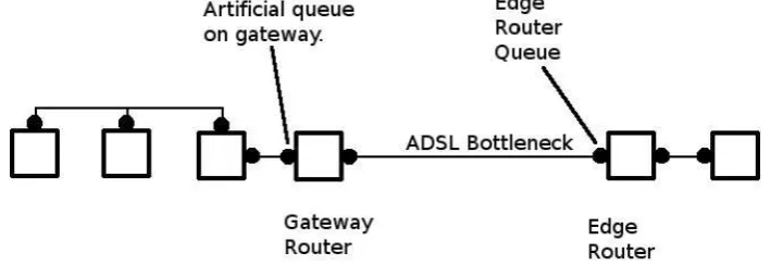
than in the core of the network, and it is possible to make a more complicated program work here without consuming an excessive amount of computing resources. In this sit-uation, most of the traffic would typically be download traffic and the bottleneck would be the ADSL modem. (See Figure 1.1.) As such, the ideal deployment for our queueing discipline would be on the edge router, the router on the internet side of the link where the download traffic is queued. But since such customers have little control over the edge router this would have to be deployed on the gateway router. For this reason, a Mice and Elephants ingress filter was created as well as a queueing discipline.

1.5

Documentation Created

A search of the internet reveals that there is little documentation publicly available on the creation of queueing disciplines. Within the Linux Kernel there is an API for queueing disciplines, but no formal documentation such as Linux man pages, Linux info pages or HOWTO exist. This project has provided documentation of the API in the form of a man page and also created a set of instructions on how to create a queueing discipline in the form of a Linux HOWTO. The HOWTO is complemented with a simple environment for queueing discipline creation and a well documented template for a new queueing discipline.

1.6

User Space Development Environment

In systems running under the Linux operating system, queueing disciplines are imple-mented in the kernel. The normal safeguards that user space programs enjoy are not present for code within the Linux Kernel. A loose pointer could result in changed mem-ory in any user process in the system. Resources not released cannot be released until the next reboot. Also, debugging is difficult. It is therefore almost essential to use some sort of user space simulation of the code being debugged.

1.7

Overview

The second chapter of this document entitledActive Queue Managementintroduces Ran-dom Early Detection, Fair Queuing and the Mice and Elephants strategy.

The third chapter entitled Linux Queueing Disciplines will explore Linux’s queue-ing discipline architecture. It introduces Linux’s AQM terminology and some important Linux AQM modules. It also describes how queuing disciplines are implemented on Linux.

1.7. OVERVIEW 13

Linux used and the environment required to develop queuing disciplines, and testing that was performed.

The fifth chapter entitledTestingdescribes the methods used for load testing and pro-vides information about the efficiency of the resulting queuing disciplines. It describes some experiments that demonstrate the benefits of the created mice and elephants queu-ing disciplines. It also introduces the test harness that was used for live debuggqueu-ing and scenario testing.

The sixth chapter entitled Deployment and Configuration describes an alternative method that was considered for the control of download traffic from a gateway router.

Chapter 2

Active Queue Management

In 1986 the internet had what was described as a series of congestion collapses [49]. New algorithms put into the Berkeley Unix BSD TCP that were developed to cope with network congestion [63]. These

include:-• round trip variance estimation

• exponential retransmit timer backoff

• slow start

• more aggressive receiver ack policy

• dynamic window sizing on congestion

• clamped retransmit backoff

Testing showed that the resulting product is fairly good at dealing with congested conditions on the internet [49]. These enhancements to TCP became known as Tahoe TCP, after BSD 4.3 Tahoe [37, 51].

The outgoing packet queues on routers have to be kept small. If they were large, then the queueing delay also would be large. So if these queues become full, they drop arriving packets. TCP sources use packet acknowledgments (ack) to confirm that sent packets actually arrived. If an acknowledgment fails to arrive, then it is assumed to be because the packet was lost (or the acknowledgment was lost) due to overflowing buffers on packet routers. Thus TCP sources detects network congestion from the failure to receive an acknowledgement for a sent packet, and in response reduces its congestion window by half, effectively reducing its output. Thus, as the TCP sources slow down their traffic generation, the congestion is controlled.

16 CHAPTER 2. ACTIVE QUEUE MANAGEMENT

2.1

Random Early Detection

On a router, each network interface has a queue associated with it. Each IP packet to be sent out on an interface will wait in the queue, until it can be transmitted onto the link. The sizes of these queues are not infinite, however, and if they were, the delays would become intolerable. Thus, packets arriving at a queue that is already full, are normally discarded. This queueing behaviour is known asdrop tail.

In 1993, Random Early Detection (RED) [44] was proposed. Traffic sources normally detect congestion when queues become so full that their packets are lost. RED introduced the idea of notifying sources about congestion beforethe the queue became full by ran-domly dropping packets. The probability of dropping packets is set to zero if a queue is empty, and increased as a queue became full over a period of time. The main points of the proposal included the

following:-• Congestion can be detected at the packet sources, for instance, but it is easier and more effective to detect and act on this at the congested node.

• IP routers capable of routing large volumes of packets will typically have large queue buffers. If queues at the slowest link are full, this will result high queueing delays and have a negative impact on certain types of traffic, e.g. interactive traffic. It is therefore in our interest to ensure that these queue sizes remain low.

• The only effective feedback mechanism for retarding packets sources in TCP/IP is by utilising the TCP response to dropped packets.

• Dropping packets can help manage a queue even without a source quench feedback mechanism. It even works with non-cooperative packet sources. The following quote is from [44]:

If RED gateways mark packets by dropping them, rather than by setting a bit in the packet header, when the average queue size exceeds the max-imum threshold, then the RED gateway controls the average queue size even in the absence of a cooperating transport protocol.

• Randomly dropping packets early rather than being forced to drop packets when the queue is full avoids the phenomenon known assource synchronisation, which is when all packet sources performing a slow start simultaneously. The following quote is from [44]:

2.1. RANDOM EARLY DETECTION 17

Min

Th

Max

Th

1

Dropping Probabi

lit

y

Buf

Size

Max

P

Average Queue Size

Non-Gentle RED

1

0

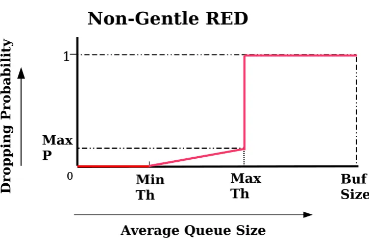
Figure 2.1: The original RED. When the average queue size exceeds the threshold thmax, then the dropping probability is set to 1.

• Design goals are:- minimise packet loss and queueing delay, avoid synchronisation of sources, maintain high link utilisation and remove biases against bursty sources.

• The average queue size is calculated using a time based exponential decay. This is so that sudden bursts of packets from bursty applications do not produce an imme-diate dropping of packets.

• Normally all packets in a given time slice will have an equal probability of being dropped. Thus the probability that a source will receive a source quench notification (dropped packet) is proportional to the number of packets the source sends.

18 CHAPTER 2. ACTIVE QUEUE MANAGEMENT

Min

Th

Max

Th

1

Drop

p

ing Pro

b

abi

lit

y

0

Buf

Size

Max

P

Average Queue Size

Gentle RED

2.2. FAIRNESS ALGORITHMS 19

A variation on the RED AQM known asGentleRED [40, 43] has been defined. Gentle RED is the same as RED except that the probability of dropping a packet follows Figure 2.2 instead of Figure 2.1. The difference between these graphs is that in Figure 2.2 the probability of dropping a packet increases linearly frommax_p at max_th to 1 at the point where the buffer is full.

Since the first paper on RED, many papers have been published on its problems, and many suggest improvements and modifications to RED. One of the problems with RED includes that of proper configuration. Improperly adjusted, the queue size of RED will typically be either empty or just under the point where the drop probability is 1. Traffic can be bursty, causing different congestion scenarios with regularity. The efficiency of RED depends on correct configuration [34, 42], and yet there is no single set of RED param-eters that work well under different congestion scenarios [33]. This leads to oscillatory behaviour that leads to packet losses when the queue is full, and network underutilisation when the queue is empty [62, 39, 41].

This problem has been solved in different ways with different mechanisms. Some of these include Stabilised RED [79], BLUE [39] Loss Ratio based RED [81], and Adap-tive RED (ARED) [41]. ARED involves using the original RED with the addition of a mechanism which constantly adjusts the most critical RED parametermaxpto achieve a target average queue length. It uses an additional measure of average queue length to that of RED, one which is more long term. If the long term average queue size is larger than the target queue size it makes the RED algorithm more aggressive by increasingmaxp. Otherwise it makes the RED algorithm less aggressive by decreasingmax_p [41]. ARED solves the problem of the oscillatory behaviour and the problem of the sensitivity of the algorithm to load [33, 57]. It is also much easier to deploy due to the fact that it requires less parameters to be set.

2.2

Fairness algorithms

In 1985 John Nagle produced an RFC entitled ”On Packet Switches With Infinite Storage” which introduced the notion of fairness amongst flows [64]. He proposed a system of multiple queues serviced in a round robin fashion. He wrote ”each source host should be able to obtain an equal fraction of the resources of each packet switch”. He did not differentiate between large multi-user hosts and small hosts or IP masquerading. This idea has come to be known asFair QueueingorProcessor Sharing.

20 CHAPTER 2. ACTIVE QUEUE MANAGEMENT

[54].

2.3

Mice and Elephants

”Mice and Elephants” and ”Shortest Job First” strategies are ones which favour the short flows over long flows. In a mice and elephants strategy the short flows or the packets from them are called mice, and the long flows or the packets from them are called elephants. The strategy involves identifying flows and associating packets with their flows in order to be able to treat long flows differently to short flows. One way to favour the mice is to give the mice priority when dequeuing. Another is to avoid dropping mouse packets by dropping elephant packets instead. This can be achieved by dropping packets early, before the queue is full.

Proponents of ”Mice and Elephants” queueing strategies argue that equal throughput for each flow or host (sometimes called ”Processor Sharing” or ”Fair Queueing”) is the wrong goal. Mice and Elephants strategy relative response times are significantly better than those obtained using Fair Queueing.

The Shortest Remaining Processing Time (SRPT) strategy is one of giving preference to the flows that have the least bytes remaining. This requires prior knowledge about the length of flows. SRPT been shown to give better results than Processor Sharing for a range of measures including average task turnover time [36, 26, 76]. Harcho-Balter, Crovella and Park [46] uses mean task turnover time divided by job length as a measure of starvation, and show that starvation of the long jobs is not an issue in internet traffic. They show both analytically and by simulation that no class of jobs are worse off when the the job sizes are heavy tailed, as they are in internet traffic.

In reality, SRPT would be difficult in a queueing discipline, because we don’t have prior knowledge of job lengths. We can only know the size of a job so far, and therefore can only implement Shortest Job First (SJF). But SJF has been shown to be a sufficiently good approximation to SRPT, to enjoy similar benefits over Processor Sharing that SRPT does. McNickle and Addie [61] show that shortest job first gives near optimal response time regardless of which group of flows we care to observe. For example, Shortest Job First gives as good a result to medium length jobs than if we were to give medium length jobs absolute priority. Simulation of an implementation of Shortest Job First is described in [17], with results that show significant gains over other strategies.

2.4. A MICE AND ELEPHANTS QUEUEING DISCIPLINE 21

the very heavy tails case 40% more capacity was required. The modelling showed that the benefit of a mice and elephants strategy would be quite significant.

Long flows constitute a small minority of flows, but carry the vast majority of bytes. About 20% of the flows have more than 10 packets but these flows carry 85% of the total traffic [74, 32]. During periods of traffic congestion the long flows account for an even greater percentage of the traffic than they do if we take overall traffic measurements. During periods of high congestion, the proportion of bytes in long flows is even greater because the long flows play a greater role in causing congestion than the short flows. In [19] an example was given where the short flows accounted for 89% of the traffic flow and the long flows accounted for the other 11% of the traffic flow overall. accounted for a disproportionate amount of the traffic flow - perhaps 88%.

It stands to reason that interactive short flows are delay sensitive as far as the per-ceived quality of service is concerned, because a human being will have an active process happening and will be impatient to wait for a result from her mouse click or keystroke. For example, the keystrokes in a telnet session will have to wait in a queue congested by packets from long flows.

It is also worth mentioning that short flows are particularly sensitive to dropped pack-ets [45]. Treating mice and elephants equally is not truly ”fair”, and it would be more fair to assist the mice in order to achieve a better perceived quality of service.

2.4

A Mice and Elephants Queueing Discipline

The Mice and Elephants Queueing Discipline constructed in this project benefits the Mice in two ways. The first way was to give absolute priority to the mice when dequeuing packets from the queueing discipline. This was most easily implemented by having two queues, one for the mice and one for the elephants.

The second way to benefit the mice is to drop elephant packets, but not mouse packets when it is necessary to drop packets. This becomes difficult if we are forced to drop packets because the queue is full, as normally happens in drop tail. We avoid this problem by using Random Early Dropping (RED). Hence we can drop a packet at any time, thus allowing us to drop elephant packets only.

It takes expertise and thought to configure RED and it is impossible to configure it to cope well for varying congestion scenarios. It is easy to provide an ARED with sensible defaults for most parameters so that it would be a relatively easy queueing discipline to configure and it automatically adjusts to changing load conditions. ARED was chosen over RED as a base for a Mice and Elephants queueing discipline for these reasons.

22 CHAPTER 2. ACTIVE QUEUE MANAGEMENT

Figure 2.3: The Premises and the Gateway Router with an extra artificial queue.

2.5

A Mice and Elephants Ingress Filter

Routers in the core of the internet must operate fast in order to handle large volumes of traffic. Tracking flows requires CPU and memory resources, and a Mice and Elephants strategy will be more difficult to implement in the core, probably requiring special strate-gies to reduce complexity, at the very least.

2.5. A MICE AND ELEPHANTS INGRESS FILTER 23

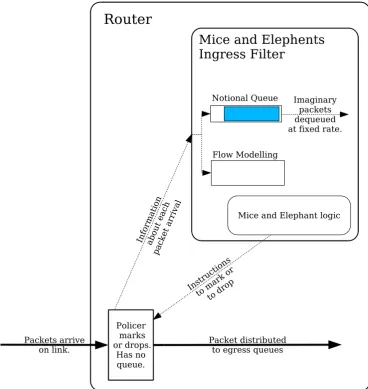
24 CHAPTER 2. ACTIVE QUEUE MANAGEMENT Policer marks or drops. Has no queue. Packets arrive

on link. Packet distributedto egress queues

Router

Mice and Elephents Ingress Filter

Notional Queue Imaginary packets dequeued at fixed rate.

Flow Modelling

Mice and Elephant logic

Instru ction

s

to ma rk or

to drop Informa tion about eac h pack et a rriv al

2.5. A MICE AND ELEPHANTS INGRESS FILTER 25

limit traffic bandwidth to a fixed value. (See Figure 2.5.) It works in the same way as the simulations in [56], but has a notional queue instead of a real one. The notional queue holds no packets, but keeps the size of the notional queue in bytes. Bytes are dequeued from the notional queue at the target bandwidth given in the configuration of the ingress filter. ARED is used to vary the marking probability of the ingress filter, just as in the queueing disciplines to achieve a fixed notional queue size. Flows are monitored just as they are in the Mice and Elephants queueing discipline, and the same strategy as is used to mark the packets belonging to elephant flows, and not mouse flows.

One could argue that a 10% slowdown in bandwidth is too high a price to pay. In many circumstances that will be true, but most often the key performance indicator is response time, not bandwidth. If interactive flows are being crowded out by large downloads, then a 10% slowdown may well be not such high a price to pay, because the perceived quality of service will be increased, i.e. the quality of service would have improved.

Chapter 3

Linux Queueing Disciplines

3.1

History of Net-4

Linus Torvolds announced that he had a working operating system in August 1991 [7, 1]. Implementation of IP handling was started 6 months later by Ross Biro [53]. Fred van Kempen started rewriting TCP/IP one year later. The project was called ”Net-2”. He was later assisted by Alan Cox, and the result was called ”Net-3”, and was available in Linux 1.0 [53]. Alex Kuznetsov wrote ”Net-4”. It was released with Linux 2.2 and is essentially what we have now in Linux 2.6 [22]. Net-4 has a flexible modular framework into which the system administrator may configure classifiers, policers and queueing disciplines for incoming or outgoing packets. Outgoing packets queue. Incoming packets do not.

3.2

Linux Networking Concepts - Classifiers, Policers,

Queueing Disciplines and Filters

Figure 3.1 shows a simple router with two network interfaces. As packets enter the in-terface on the left they are subject to apolicer. A policer in this context, has the power to drop or mark any packet that it chooses. It cannot, however, queue any packets. In this example, packets that are not dropped are delivered to the queueing discipline on the right.

Unlike policers, queueing disciplines, have one or more queues in which to queue packets. When a packet is delivered to a queueing discipline, it may drop, mark, or queue the packet. It may even choose to queue this packet, and drop another already queued. When a network interface is ready to send, the queueing discipline is asked for a packet. The queueing discipline will normally satisfy the request by dequeuing one packet. Figure 3.2 shows the flow of packets through a queueing discipline.

Queueing disciplines may beclasslessorclassfull. A classfull queueing discipline is

28 CHAPTER 3. LINUX QUEUEING DISCIPLINES

Linux Router

Network

InterfaceNetwork InterfaceNetwork Interface

Policer

Queuing Discipline

Queuing Discipline

Policer

Figure 3.1: A Linux router with two network interfaces, each with a policer and a queue-ing discipline.

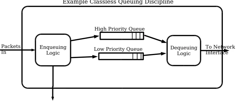
Example Classless Queuing Discipline

Enqueuing

Logic DequeuingLogic High Priority Queue

Low Priority Queue Packets

In To NetworkInterface

3.2. LINUX NETWORKING CONCEPTS - CLASSIFIERS, POLICERS, QUEUEING DISCIPLINES AND FILTERS29

Dequeuing Logic P

l u g Plug in Classifier

Plug in Queuing Discipline

Plug in Queuing Discipline

Classfull Queuing Discipline

30 CHAPTER 3. LINUX QUEUEING DISCIPLINES

one that is a container for child queueing disciplines and uses a classifier (alternatively called a filter) to decide which inner queueing discipline to send incoming packets to. Figure 3.3 shows the flow of packets through a classfull queueing discipline. The clas-sifier and inner queueing disciplines of a classfull queueing discipline are specified as configuration [21].

In Linux, the policer is formed by combining a classifier with the the specialingress queueing discipline. Normal queueing disciplines are sometimes referred to as egress queueing disciplines because they deal with packet departures from a network interface. The so called ingress queueing discipline deals with packet arrivals. Figure 2.5 shows the flow of packets in a policer. Thus classifiers may be used to direct packets within classfull queueing disciplines, or they may be used decide when to drop packets. Policers are optional, and by default will not be used.

Queueing disciplines that manage packets without the use of child queueing discipline are called classlessqueueing disciplines. Eventually, an enqueued packet must reach a classless queueing discipline. Algorithms from the field of Active Queue Management, such as ”Drop Tail”, ”RED”, ”SFQ” are implemented in classless queueing disciplines.

To summarise, outgoing packets to an interface will go to a queueing discipline. This could be the default, which would be a simple drop tail queueing discipline, or the system administrator may have specified an advanced queueing discipline (for example SFQ), or it could be a classfull queueing discipline. Such a classfull queueing discipline would be a container for classes, filters (which will direct packets to classes), and ultimately queueing disciplines. These queueing disciplines may themselves be classless or classfull.

3.2.1

U32

An example of a classifier is ”U32”. It allows you to specify tests on packet headers. A packet that passes of all of those tests will be sent to a specified class, which may be an instance of a queueing discipline. The tests of U32 have two parts, - a mask which specifies what bits of the packet header get tested and a value that the tested bits must match in order to pass. This may seem to be rather limited, but in practice it is quite powerful, allowing the system administrator to send different types of service to different queues, or to treat ”syn” packets differently [15].

3.2.2

HTB

3.3. KERNEL MODULES 31

Two properties associated with each class are the minimum and maximum bandwidth for dequeuing [30]. HTB attempts to satisfy the minimum dequeuing bandwidth first. It may not succeed if the interface (or the next level up class) is too slow. If it does not succeed, then it dequeues from each class in proportion to the minimum bandwidth of each class. If, on the other hand, it does satisfy the minimum bandwidths of each class, and there is yet more bandwidth available, it will allocate to each in proportion to the maximum bandwidths. It will not deliver more than the maximum bandwidth to any class.

3.3

Kernel Modules

Linux queueing disciplines and classifiers may be compiled directly into the kernel, but for development it ismuchmore convenient to use a kernel module. One can compile a kernel module alone and insert it into the kernel for testing. One is then able to remove the module from the kernel for further modifications. If, on the other hand, you chose to compile into the kernel directly you would have to reboot the computer in order to try modifications. Kernel modules are also better for the system administrator because the modules that are not used will not be loaded, and therefore will not increase the size of the kernel. Loadable kernel modules make the framework for Linux queueing modules much more flexible. Loadable modules first appeared in Linux 1.2 in 1995 [47], but were greatly enhanced with in Linux 2.0 in 1996, with the introduction of automatic kernel loading and module dependency handling [8].

3.4

The Linux Queueing Discipline Interface

The Linux kernel has a well defined, but poorly documented interface for queueing disci-plines. I have written a Linux man page in order to fully document the interface. This is included Appendix B.

3.5

Setting up a Linux Queueing Discipline Interface

The system administrator sets up, configures, and removes queueing disciplines from network interfaces using the linuxtc command [10]. tcstands for Traffic Control. It is necessary to extend tcwhen providing a new queueing discipline. The use oftc is best explained in the ”Traffic Control HOWTO” [29]. A generously commented script using thetccommand that I used for testing my queueing disciplines is provided in Appendix G.

32 CHAPTER 3. LINUX QUEUEING DISCIPLINES

Chapter 4

Implementation

4.1

Summary of Queueing Disciplines Developed

4.1.1

Drop Tail

As a first step in the implementation of Mice and Elephant queueing disciplines, I imple-mented the simplest possible Linux queueing disciplinedrop tail. The drop tail queueing discipline was created as learning step rather than an end goal in its own right. Creation of this most simple queueing discipline demonstrated running code that utilised Linux’s queueing discipline framework. Later, the drop tail queueing discipline was modified and heavily commented to turn it into a template for the development of queueing disciplines, as a companion to the queueing discipline how-to, delivered as part of this project.

4.1.2

RED

This code was then re-used in the creation of a RED queueing discipline. As Linux already has a RED queueing discipline, this was not useful as an end deliverable, but it was useful in that it could be tested, and the code could then be re-used for the next step.

The RED algorithm is a mechanism which marks or drops packets before the queue is full. Its configurations defines two dropping thresholds min_th and max_th. When the average queue size is less thanminth, no packet dropping occurs. When the average queue size is betweenmin_th and max_th, then a packet dropping probability applies as shown in the Figure 2.2. When the average queue size is greater than max_th then the dropping probability is applied as in Figure 2.2, depending on whether the gently variety of RED is being used.

The basic algorithm of RED, which follows, is directly quoted from [44]:-for each packet arrival

calculate the average queue sizeavg

34 CHAPTER 4. IMPLEMENTATION

ifmin_th≤avg<max_th calculate probability pa with probability p_a:

mark the arriving packet else ifmax_th<=avg

mark the arriving packet

In order that the queue size that results from bursty traffic or from transient congestion does not result in a significant increase in the average queue size, the average queue size calculated by means of a weighted exponential running average of the queue length as follows

:-avg←(1−wq)avg+wqq

A time based weighted exponential should be updated at regular time intervals. For ef-ficiency considerations, however, this is actually updated at each packet arrival. There would be a problem here if the queue has been idle. In this case our formula would not take into account the idle time at all. That is why the following formula is used instead if a packet arrives at an empty queue

:-m←(time−qtime)/s avg←avg(1−wq)m

Wheresis the average transmission time for a packet,timeis the current time, andqtime is the start of the queue idle time.

The dropping probability pais calculated in two stages as follows:-p_b←max_p(avg−min_th)/(max_th−min_th)

Then the packet marking probability p_ais dependant on the count of packets since the last marked

packet:-pa←pb/(1−count pb)

4.1.3

ARED

The next queueing discipline developed was an Adaptive RED (ARED) queueing disci-pline. Unlike RED, there is no ARED distributed with the Linux kernel. Therefore it is of significant value to provide an implementation of ARED for Linux.

4.1. SUMMARY OF QUEUEING DISCIPLINES DEVELOPED 35

[62, 39, 41]. Adaptive RED solves this by dynamically configuring RED’s most critical configuration parameter.

The algorithm that achieves this is simple. The following definition of ARED is taken from Floyd, Gummadi and Shenker

[41]:-Every (interval) seconds:

if ( avg>target max_p≤0.5 )

maxp←maxp+α{increasemaxp} elseif ( avg<target max_p≥0.01 )

max_p←max_p×β{decreasemaxp}

where

avg is average queue size

interval is the time between adjustments. 0.5 seconds is recommended.

target is the desired average queue length. Half way betweenmin_thandmax_th is recom-mended.

α is the amount to increasemaxpby, andmin(0.01,maxp/4)is recommended.

β is the amount to multiplymaxpby in order to decrease it. 0.9 is recommended. A manual page for the ARED Linux queueing discipline is included in Appendix C.

4.1.4

Mice and Elephants

A Mice and Elephants queueing discipline associates packets with a flow, and these flows are classified as being small (mouse flows) or large (elephant flows) depending on whether the length in bytes (or possibly the length in packets) is smaller or larger than a given constant threshold.

The Mice and Elephant queueing discipline has two queues, an elephants queue for packets associated with elephant flows and a mouse queue for packets associated with mouse flows. Packets in the mouse queue are given absolute priority over packets in the elephants queue.

36 CHAPTER 4. IMPLEMENTATION

Two different Mice and Elephant queueing disciplines were produced. meredis sim-ply as described above. meredt is configurable so that it behaves as mered does, but features a more flexible configuration so that it may be made to perform fair queueing, for example. Manual pages for these queueing disciplines are provided Appendix D and Appendix E.

4.1.5

Mice and Elephants Classifier

This contribution to Linux is aimed at incoming packets from a network interface rather than a queue for outgoing packets.

Taking the case of a typical domestic residence or small business, the bottleneck is the link entering the premises, as shown in Figure 1.1. Typically, most of the network traffic across the link is in the downloaddirection, coming from the internet into the premises. Therefore, in order to control this downward traffic, it would be best to place a queueing discipline on the edge router, i.e. the router on the internet side of the link. Sadly the owner of the premises has little control over the edge router.

One way of controlling the traffic over this link is by means of a policer. There is no queue here, but a policer may selectively mark or drop packets entering an interface. Thus if deployed on the gateway, it can be used to control downward flows.

The Mice and Elephants classifier works with the Linuxingressqueueing discipline to form a policer that will favour packets associated with mouse flows over packets associ-ated with elephant flows. This policer works by simulating an artificial bottleneck, which is explained in section 2.5. If the overall bandwidth arriving from the interface exceeds a given threshold, then this policer attempts to reduce the flow to the threshold by marking or dropping packets. It is a Mice and Elephant policer, because it keeps flow records and prefers to drop packets from mouse flows rather than packets from elephant flows.

As explained in section 3.2, the policer can mark packets, drop packets or permit their passage, but it cannot retain or queue packets, so we cannot have a real queue here. Instead, we keep a virtual or imaginary queue, that holds no packets. It has only a number holding the queue size in bytes. For each real packet arrival, an imaginary packet of the same size is added to our virtual queue. At the same time, in order to simulate dequeueing, the size of the queue is decreased by the target bandwidth multiplied by the time since the last packet. Packets are marked or dropped as indicated by the ARED algorithm which will base its decisions on the size of the virtual queue, rather than the size of an actual queue.

4.2. DESIGN DETAILS 37

4.2

Design Details

4.2.1

RED

The coding used in Linux’s RED queueing discipline is, like much kernel code, highly optimised. There is not a direct one to one correspondence between the published RED al-gorithm [44] and the coding in Linux’s RED queueing discipline. The programmers have found approximations to the published algorithm that are computationally faster. These same optimisations make Linux’s RED difficult to understand and even more difficult to extend. Thus, it was considerably easier to write my own RED from scratch using the published algorithm.

The code in Linux’s RED avoids floating point arithmetic within the Linux kernel, preferring to implement fixed point arithmetic using integers. I did not take that approach because I believe it to be outdated. Once, integer arithmetic was much faster than floating point arithmetic, but modern CPUs come equipped with fast floating point processors, and the Pentiums found in modern PCs are no exception [82, 80, 68]. On modern Pentiums an integer multiply takes 4/7 CPU cycles. That means it will take 4 cycles from the beginning of an integer multiply instruction till the next CPU instruction can begin, but the result of the operation wont be available until 7 CPU cycles. A floating point multiply takes 1/3 CPU cycles, which is at least twice as fast as the integer multiply [82, 80]. My approach was to not care about the CPU times for these operations, i.e. to use floating point or integer arithmetic wherever it was most convenient.

One of the creators of RED, Sally Floyd, has since recommended the gentle variety of RED [43]. I chose to implement the gentle variety of RED.

The published algorithm for RED suggests the use of auniformrandom variable for intermarking times as opposed togeometricrandom variable for intermarking times [44]. By way of explanation, this means that it uses a random number generator to establish a count of packets until the next packet dropped, rather than apply a dropping probability to each individual packet. Floyd and Van Jacobsen claim that this is preferable as applying a dropping probability to each individual packet can result in too many dropped packets close together or alternatively, too long an interval between marked packets. Linux’s RED queueing discipline uses this suggested uniform random variable, and my RED does also.

Smoothed Estimate of Queue Size

Ideally, the estimate of the queue size should be updated at regular time intervals. This would cause extra computational overhead, as this can be approximated in other ways. The RED algorithm [44] specifies a practical method of calculating the average queue size, and I have used this method with some improvements.

38 CHAPTER 4. IMPLEMENTATION

updated

by:-avg←(1−w)avg+w×qsize

where avgis the average queue size,qsize is the current queue size and wis a constant which controls the weighting of past history verses current queue size.

If there are no packets in the queue on a packet arrival, then the average queue size will be calculated according to how many packets might normally have arrived in the period of time since the last packet arrival. Thus the following assignment is used

:-avg←avg×(1−w)(time−qtime)/s

wheretimeis the current time,qtimeis the time of departure of the last packet, and sis the average transmission time. For convenience I will call the term used to multiply the average queue size theaverage queue size multiplier.

Floyd and Van Jacobson [44] recommend that the raising of power be achieved by means of a table. In Linux’s RED, this table is implemented grudgingly. The following quote is from comments in the code of Linux’s

RED:-This is an apparently over-complicated solution (i.e. we have to precompute a table to make this calculation in reasonable time) I believe that a simpler model may be used here, but it is field for experiments.

I agree with the author’s sentiments. I implemented that part by approximating the exponential curve with a quadratic equation over the relevant part of the curve. RED’s al-gorithm for estimating the average queue size is only an approximation, and my quadratic fit is an approximation to that.

I use the further simplification that once sufficient time has passed and therefore the average queue size multiplier is close enough to zero, I do not do a calculation at all. I simply set the average queue size to zero. Let f be the size of the average queue multiplier at this point where I regard it as sufficiently close to zero.

Letxbe the number of packets that might normally have arrived in the period of time since the last packet. Since we have to choose an arbitrary rate of packet arrival, x is synonymous with time. Let

v=1−w Letx0be the number of packets such that

vx0_{= f}

then

x0= ln(f)

ln(v)

My quadratic approximation has the form

4.2. DESIGN DETAILS 39

wherey is the number to multiply the the new average by. In order to select a suitable quadratic approximation, I chose to select intuitive boundary conditions, which should ensure that it is accurate in the region of interest. These boundary conditions are sufficient to dictate the parameters of the quadratic approximation.

The first boundary condition is important: When no time has passed, then there is no reduction in the average queue size, i.e.

y(0) =1

The next ensures that the curve is continuous. Recall that we use the simplification that we use 0 whenxis greater thanx₀: The average queue size should be set to 0 atx₀, i.e.

y(x₀) =0

The last prevents the curve from dipping below 0 whilexis less thanx₀, and give the most curvature: The curve should be flat atx0, i.e.

y0(x₀) =0

From this I derived the coefficients of my quadratic equation. The quadratic equation

became:-y= 1

x₀2∗x 2₋ 2

x₀∗x+1

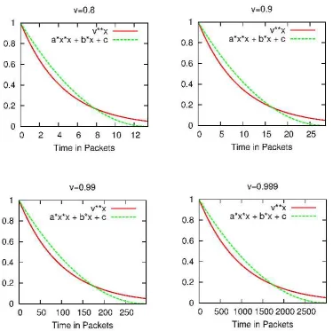
I plotted the results for various values of f and by trial and error found that a value of f which keeps the approximation close to the exponential curve was ₁₅1. Figure 4.2.1 shows my quadratic approximation together with the exponential curve as per the published RED algorithm for various values of v. It shows that the approximation is valid regardless of the value ofvorw. In each of these graphs the two curves cross each other aty=0.2779.

4.2.2

ARED

I directly implemented the algorithm as described by Floyd, Gummadi and Shenker [41]. I also implemented their suggestions for setting the parameters, so now most of my ARED parameters have good default values. There are only three parameter that a system ad-ministrator should set, and these do not require an understanding of ARED. These are the queue length, the Maximum Transmission Unit (MTU) and the speed of the interface. The last two parameters could potentially be discovered automatically, but that is work that I have not undertaken.

4.2.3

Mered - The First Mice and Elephants Queueing Discipline

40 CHAPTER 4. IMPLEMENTATION

4.2. DESIGN DETAILS 41

having two queues. Packets in the queue that the mice packets go into will have absolute priority over packets in the Elephants queue.

The second way to preferentially treat mice packets is to attempt to give the mouse packets immunity from being dropped. As explained earlier I use a random number gen-erator to establish a count of packets that will be accepted before dropping a packet. If the count is up, thus indicating that the current packet should be dropped, then I drop it only if it is an elephant packet. Dropping is suspended until either an elephant packet arrives or the queue gets too full to accept more packets. Hopefully the latter case is rare.

In order to preferentially treat mouse packets, I have to be able to tell between mouse packets and elephant packets. To do this I keep track of the flow for each packet and keep a count of the number of bytes of each flow. If a flow has had less than a given threshold of bytes then all packets belonging to that flow are classified as mouse packets. Otherwise packets belonging to that flow are classified as elephant packets. I keep not just one mouse/elephant threshold, but two. One is for classification as mice for the purpose of dropping and the other is for classification between mice and elephants for the purpose of queueing.

Hashing of Flow Records

In this Linux queueing discipline, flows are identified by some combination of source and destination IP numbers (as well as the source and destination port numbers in the case of TCP or UDP packets). These values are extracted from each packet, and then a mechanism is used to quickly find the records for the flow associated with the packet.

Any one of a range of mechanisms such as a tree or Bloom [27] filter or bucket mecha-nism similar to that used in SFQ [60]. I chose to use traditional hashing technique because it simple and also fast in execution. The IP and port numbers themselves are not kept in each flow record. Only the hashed value is kept. This reduces the storage space associated with each flow record and CPU time needed to compare the flow of the flow record with the flow of the packet.

For distinct flows to be distinct, it is desirable for the hashing function to be of good quality. A good quality hashing function will approximate uniform hashing [83, 65]. If we use uniform hashing or a hashing that approximates uniform hashing, the probability of packet misclassification will be tiny. The probability of any two flows having an equal 32 bit hash value will be will be the same as the probability of any two random 32 bit integers being equal, which is 1

232 . The probability that no two flows hash to the same

value would be

:-n−1

∏

(N−i

N )

42 CHAPTER 4. IMPLEMENTATION

unlikely event of packet misclassification would not be a disaster we need not worry. I considered three separate hashing functions. The first hashing function, which I will call hash1 is based on one given in Kernighan and Ritchie [52]. In it, we set Ato some initial starting value, and then we do the following for each byte of the

key:-A←(A∗m+ch)MOD M

where A is the hash value, m is some large number co-prime with M , ch is the next byte from our key andM=232 . TheMODoperation happens automatically by integer overflow. My concern was that because this operation happened for each byte this might be slow. This has 4 add operations and 4 multiply operations when used on a 32 bit words. When used to distinguish flows, this has to be done at least 3 times, so that is 12 adds and 12 multiplies, 24 operations in total.

The second hashing function, which I will call hash2, is based on the one used in Linux’s SFQ queueing discipline [60]. We setAto some arbitrary value, and then do the following for each four byte word of the

key:-A←(A16+A∗m)⊕b4MOD M

whereAis the hash value,mis some large number co-prime withM,b4 is the next 4 byte word of our key and M =232 . The MODoperation happens automatically by integer overflow.

To put it in words, for each four bytes, the current hash value is recreated by adding a shifted right version to a multiplied version of the hash value. The result is then exclusive OR’d with the 4 byte value being incorporated into the hash. I use power of two modulus in my arithmetic for the sake of efficiency.

The third hash function considered waslookup2[50].

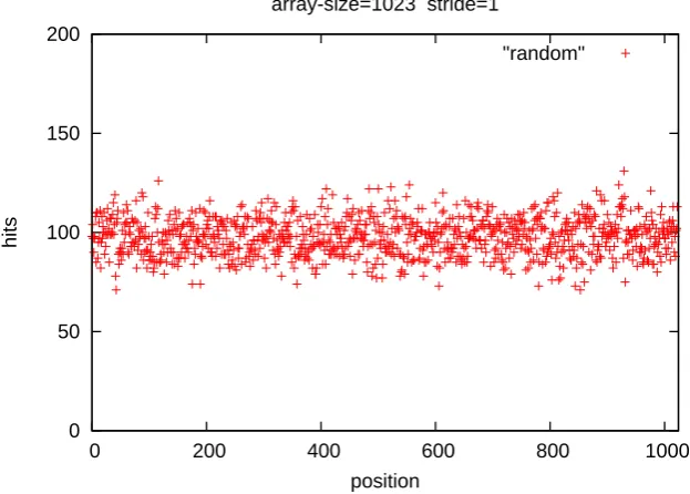
The data that I wanted to hash are the IP protocol, the source and destination IP and port numbers associated with a packet, i.e. several short pieces of data. In order to get some idea of the quality of hashing, I started with a data value of 0 and incremented by the value which I called the ”stripe”, in order to explore interesting data values. I used my hashing algorithms to obtain a hash value of each resulting data value. I then used the hash value to index an array by using the modulus operator and increment the array element whenever I got a hit. I plotted the hit counts verses the array index.

I would expect a good quality random number generator, and a good quality encryp-tion algorithm would both give a very good approximaencryp-tions uniform hashing and I used them as a control to show me what these ought to look like under uniform hashing. I used blowfish encryption [73] for my encryption. For the random number generator I used the UNIX successor to the ANSI C random number generatorrand, calledrandom[14].

4.2. DESIGN DETAILS 43 0 50 100 150 200

0 200 400 600 800 1000

hits

position

array-size=1023 stride=1

"random"

Figure 4.2: Hit count of hash table index. This plot was generated using the UNIX successor to the ANSI C random number generatorrand, calledrandom.

As having an array size of a power of two appears to be the worst case scenario, and the most interesting, I will present examples from this case.

Figure 4.3 and Figure 4.2 are provided as a reference to compare our hash functions to. Figure 4.4 shows the hit count of array indices for hash1. It shows a very smooth distribution, and a pattern is visible under closer inspection. It could potentially be a good hashing function, but it is clearly distinguishable from normal hashing. Figure 4.5 shows the hit count of array indices for hash1. Most hash indices have not been hit at all, and many that have been hit, have been hit 5 times more than the average hit rate. Figure 4.6 appears to be consistent with normal hashing.

These results seem to indicate that if random and blowfish are consistent with uniform hashing, then both hash1 and hash2 are inconsistent with normal hashing. Hash2, in particular would make a poor hashing function. Lookup2, on the other hand, appears to be consistent with normal hashing.

It is also important for the hashing to be efficient. My experimentation involved per-forming the hash as if on a flow key 100 million times on my 1200MHz AMD Duron Pentium PC. I used the hash function in-lined 10 times in the innermost loop to drown out looping overheads. Hash1 took 2.25 seconds. Hash2 took 0.723 seconds. Lookup2 took 1.35 seconds.

44 CHAPTER 4. IMPLEMENTATION 0 50 100 150 200

0 200 400 600 800 1000

hits

position

array-size=1023 stride=1

"blowfish"

Figure 4.3: Hit count of hash table index. This plot was generated using the blowfish encryption algorithm as a hashing function.

4.2.4

Meredt - The Second Mice and Elephants Queueing Discipline

The creation of the first mice and elephants queueing discipline, mered, represented the achievement of a milestone in the evolution plan. A second mice and elephants queueing disciplinemeredt was created that would have the flexibility that is typically required of useful products. The additional functionality ofmeredt over and above that of mered is described below.

Flow Sizes and Queue Size Measured in Bytes

4.2. DESIGN DETAILS 45 0 50 100 150 200

0 200 400 600 800 1000

hits

position

array-size=1024 stride=1

"hash1"

Figure 4.4: Hit count of hash table index. This plot was generated using hash1 as a hashing function.

Flexible Flow Weightings

In a domestic situation where there was an interactive telnet session competing for band-width with people using a graphical web browser, then the telnet session would constitute a mouse flow, and the web browser would constitute an elephant flow. Alternatively if the web browser was competing for bandwidth with a large download, then the web browser would constitute a mouse flow, and the download would constitute an elephant flow. In my mind at least, mice and elephants are relative descriptions, so by default the second Mice and Elephants queueing discipline allows flows to become elephants gradually, instead of having a single hard threshold.

The configuration optionally includes a piecewise linear function that maps actual flow size to flow length weighting. Thus, the system administrator need not accept the default behaviour.

46 CHAPTER 4. IMPLEMENTATION 0 50 100 150 200

0 200 400 600 800 1000

hits

position

array-size=1024 stride=1

"hash2"

Figure 4.5: Hit count of hash table index. This plot was generated using hash2 as a hashing function.

the dropping probability of a packet will be proportional to the flow length weighting of its flow. This way, depending on the piecewise linear function given in the configuration, mouse flows are not subject to dropping but elephant flows are.

If the average dropping probability provided by ARED and the average flow length weighting are relatively stable, then it is easy to show that the average of the dropping probability actually applied is the average dropping probability provided by ARED. The applied dropping probability for the packet p_pis given by the following

formula:-p_p=p_r∗ wp

w_av

wherepris the dropping probability supplied by ARED,wpis the flow length weight-ing for the packet, and w_av is the maintained average flow length weighting. Thus the average of the dropping probability applied is given

by:-E(p_p) =E(p_r∗ wp

wav

)

= pr

w_av∗E(wp)

= p_r∗wav

4.2. DESIGN DETAILS 47 0 50 100 150 200

0 200 400 600 800 1000

hits

position

array-size=1024 stride=1

"lookup2"

Figure 4.6: Hit count of hash table index. This plot was generated using lookup2 as a hashing function.

=pr

There may well be occasions when the dropping probability for the packet p_pis cal-culated to be greater than 1. In this case, the packet will be marked or dropped, effectively making p_p equal to 1, thus breaking the relationship E(p_p) =p_r . Because this cannot happen in a sustained way, and so should be rare, the average dropping probability applied will still be approximately equal to the dropping probability provided by ARED,

It is worth noting that flexible flow length weightings allow the system administrator to implement a strategy that is more consistent with Shortest Job First than Mice and Elephants queueing.

Fair Queueing Hybrid

A mice and elephants queueing discipline classifies flows according to their length in bytes or packets. Once a flow has been classified as being large, it will always be regarded as a large flow. A fair queueing discipline, on the other hand classifies flows according to their current behaviour.

48 CHAPTER 4. IMPLEMENTATION

by a value derived by dividing the link capacity by the total number of active flows and then multiplying by the fair queueing factor. In other words, a flows perceived size will slowly reduce if it is relatively inactive and thus the perceived size reflects the flow rate rather than its length. This factor is zero by default, so that by default the queueing discipline is a pure Mice and Elephants queueing discipline. If it is 1 or above, and the mice and elephants threshold is low, then this queueing discipline will provide fair queueing. If this factor is between 0 and 1, then this is a hybrid between fair queueing and mice and elephants.

Flexible Definition of Flows

The default definition of a flow is the TCP definition of a flow or TCP connection (i.e. source and destination IP numbers together with source and destination port numbers). Although there is no such thing as a UDP connection, the same attributes can be used to define a UDP flow. If the source port of a UDP packet is non zero then it indicates the port to which a reply should be addressed [69].

It is clear that the TCP definition of a flow is not always suitable. If we wished the definition of flows to be the computer to computer traffic, for example, we can do this by using only the source and destination IP numbers. Another example of a flow might be all the traffic associated with a human activity.

This queueing discipline optionally permits the system administrator to configure it to use the source IP address, the destination address, the source port number, the destination port number, the protocol or any combination of the above as the flow definition.

Flexibility in Marking or Dropping Packets

The default action is to drop targeted packets. This queueing discipline may optionally be configured to mark packets using explicit congestion notification or it may be configured to drop them. It may also be configured so that it will mark targeted packets if they are ECN capable and drop them if they are not.

4.2.5

Meredtf - The Mice and Elephants Ingress Filter

Recall from section 4.1.5 that the mice and elephants ingress filter can be used in the gateway router at the entrance to a premises to control the download traffic that normally dominates the link.

4.3. QUEUEING DISCIPLINE DEVELOPMENT ENVIRONMENTS 49

4.3

Queueing Discipline Development Environments

If I run a program under Linux, I am running it under an environment which I will call ”user space”. I will call such a program a ”user space program” or just a ”process”.

There are various safeguards available to you when you run a program in user space. If your program accesses memory that it should not, the kernel stops your program at that point. You can even get the kernel to create an ”image” at that point for debugging. Your program is prevented from accidentally damaging the memory of other processes. Other exceptional conditions such as division by zero will cause a similar action. The allocated resources of a user space program such as computer memory will be automati-cally released by the kernel upon termination of the program. The user has the option of terminating a user space program. Also, it is easy to create and control diagnostic output from a user space program. In addition, debugging tools will let you open a user space program and allow you to inspect or to modify memory within it.

The Linux kernel is the program that provides this ”User Space”, but for the kernel itself there are no such safeguards and little in the way of debugging tools. If you run code directly in the Linux kernel, a pointer with a bad value is likely to crash your computer, if you are lucky. In this case you will have to perform a time consuming reboot of the computer. There is no saying what might happen if you are unlucky. Sometimes such errors have caused random writing to the hard drive. It is therefore almost essential to use a user mode environment in order to test AQM code as it is being developed.

There are a some publicly available schemes which may be employed to run queueing disciplines in user space and descriptions of them follow

below:-4.3.1

Tcsim

The traffic control simulator (TCSIM) [23] can be used to test a queueing discipline. TCSIM allows one to drive a queueing discipline under the control of a script. It may well be a very simple script that fires one packet per millisecond, or it may be more complicated and do things like have several packets arrive at once, for example. The script controls the enqueuing of packets as well as the dequeuing of packets [16].

The language for the script provides full control over the length of the packet and the contents of each packet. TCSIM has include files which provide offsets and widths for the fields of IP, TCP, UDP and ICMP. These make it easy to specify just what should go into a packet.

50 CHAPTER 4. IMPLEMENTATION

A limitation of this scripting language is that it is not two way. TCSIM doesn’t have the ability to respond to traffic. It has a ”poll” command which dequeues packets, but the poll command does not return information to the script. Nor does TCSIM have the ability to simulate the receiving application’s response to packets. TCSIM can only generate packets and monitor the effects in the queueing disciplines.

In reality there is a two way interaction, that is, the behaviour of a TCP source is dependent on the acknowledgements. The arrival of TCP/IP packets at a router is de-pendent on the history of each routers treatment of previous packets. Therefore, no pre-arrangement of packets will be a satisfactory simulation of TCP/IP traffic. Give that TC-SIM can only generate pre-arranged sequence of packets, I would not recommend TCTC-SIM for realistic traffic simulations.

TCSIM replicates a substantial quantity of the Linux network stack in order to call the queueing disciplines. In [24] the creator of TCSIM, Werner Almesberger offers the following

justification:-Simulators usually implement an abstract model of the system they simulate. In the case of TCNG, this approach could lead to a simulator that contains the same mis-interpretations as the program being tested, so both would happily agree on incorrect results. To avoid this problem, TCSIM reduces the amount of abstraction needed by building the simulation environment from portions of the original traffic control code of the kernel, and the tc utility.

I used TCSIM and tried out some of the built in queueing disciplines. I found it rela-tively easy to accomplish. I also built and ran my mice and elephants queueing discipline in it. It was not so easy, however, to integrate my queueing discipline into it. There is a fairly large directory tree to compile, and the makefile did not properly clean away some libraries from an old compile. When I did understand enough about it to remove the old libraries, my queueing discipline integrated into TCSIM as it should according to the doc-umentation. I regard TCSIM as a feasible way of testing queueing disciplines, once the developer has learned how to use this environment.

4.3.2

User Mode Linux

The Linux kernel has been ported so that it runs in user space, and the result has been called User Mode Linux (UML) [78]. Hardware calls for the hosted Linux operating system are implemented as system calls into the host operating system. UML allows one to debug any modifications to the Linux kernel in user space. The result is called User Mode Linux. Applications in general do not have to be ported or even recompiled in order to run under User Mode Linux.

:-4.3. QUEUEING DISCIPLINE DEVELOPMENT ENVIRONMENTS 51

• Hostile or insecure or potentially hostile or insecure applications can be monitored and run safely in a virtual operating system with its own file system.

• Users or applications can be allocated a set amount of system resources.

• You could use it to test Debian verses Redhat all on the one machine without re-booting.

• Although this uses Linux as the host machine, it would be relatively easy to port this virtual operating system to run natively under other operating systems. It is relatively easy to run UML on other Unix systems, so far this has not been run under Windows.

• One of the popular uses for UML is for web hosters. Web hosters can now lease virtual machines complete with the root password. Examples of this are :- [11] [4] [2] [6]

• Virtual local area networks can be set up and prototyped.

I have not installed UML, let alone attempted to use it to develop Linux queueing disciplines. I instinctively felt that this would probably be a project in itself, and my time constraints would not permit this.

4.3.3

Umlsim

With UML, it is possible to set up virtual networks and try them out. It is also possible to perform user space debugging on the kernel. UMLSim [13, 24] takes this further by providing a language that specialises in debugging processes and in specifying and setting up network experiments. It modifies UML in order to enable debugging and to control the Linux’s idea of the time.

UMLSim has a very powerful language which features user defined routines, types and objects. It also has the capability to debug programs set breakpoints in programs, examine variables, force function calls or returns, all in an automated fashion as part of the language. UMLSim places the perceived time of the UML instances under control of the language. The language can disable the normal incrementation of time, and set the time explicitly itself as it needs. It can quickly create virtual Linux instances on a real machine, and carry out experiments.

Despite richness of this AQM simulation environment, it concerned me that traffic simulations are one way only. Return ”ack” traffic is not simulated as a part of this. It would not be easy to monitor ”real” traffic generated by applications in the way that one could using UML alone.

52 CHAPTER 4. IMPLEMENTATION

as befits a hacker’s toy, documentation is incoherent and spotty” [24]. As such I did not think that my project was big enough that I could afford to spend enough time learning about this environment to use it profitably. In a large project, I suspect that the ability to set up live traffic in the way that one could with UML alone, would make the use of UML a better option.

4.3.4

Linquede

Ultimately, I used a fairly simple scheme in order to test my AQM code in user space. The AQM code is linked in two different ways by two different makefiles. One of them compiles and links the queueing disciplines into a Linux kernel module that can be run live in the Linux kernel. The other links into a user space test harness that drives the queueing disciplines according to data provided in the form of ASCII text files. This scheme grew into a small queueing discipline development environment, which I called Linquede.

In addition to the linking and running in user space, Linquede provides a well doc-umented queueing discipline template that after installation and running the setup script will compile in