An effective integrated-RBFN Cartesian-grid discretization for the stream function-vorticity-temperature formulation in nonrectangular domains

An effective integrated-RBFN Cartesian-grid

discretisation for the stream

function-vorticity-temperature formulation in

non-rectangular domains

K. Le-Cao, N. Mai-Duy

and T. Tran-Cong

Computational Engineering and Science Research Centre

Faculty of Engineering and Surveying

The University of Southern Queensland, Toowoomba, QLD 4350, Australia

Submitted to

Numerical Heat Transfer, Part B

, 11-Dec-2008; revised,

22-Jan-2009

Abstract This paper presents a new numerical collocation procedure, based on Cartesian

grids and one-dimensional integrated radial-basis-function networks (1D-IRBFNs), for the

simulation of natural convection defined in two-dimensional multiply-connected domains and

governed by the stream function - vorticity - temperature formulation. Special emphasis is

placed on the handling of vorticity values at boundary points that do not coincide with grid

nodes. A suitable formula for computing vorticity boundary conditions, which is based on the

approximations with respect to one coordinate direction only, is proposed. Normal derivative

boundary conditions for the stream function are forced to be satisfied identically. Several test

problems, including natural convection in the annulus between square and circular cylinders,

are considered to investigate the accuracy of the proposed technique.

Keywords: Integrated radial-basis-function networks; Non-rectangular domains; Cartesian

grids; Stream function - vorticity - temperature formulation; Vorticity boundary conditions.

NOMENCLATURE

CM convergence measure R radius of inner circle

Di diameter of inner cylinder Ra Rayleigh number

Do diameter of outer cylinder s arc length

g gravitational acceleration t tangential direction/time

gi(x) radial basis function T temperature

h grid size u, v x andy components of velocity

H side length of outer square w RBF weight

I_i(.)(x) integrated radial basis function x, y coordinates

k thermal conductivity α thermal diffusivity ¯

keq average equivalent conductivity β thermal expansion coefficient

L distance between two cylinders ν kinematic viscosity (= (Do−Di)/2) ψ stream function

n normal direction ω vorticity

nip number of interior points Subscripts

N e discrete relativeL2 error b boundary value

N u average Nusselt number e exact solution

1

Introduction

Natural convection, where the motion of a fluid is caused by the combination of density

variations and gravity, can be governed by the coupling of the momentum (velocity field)

and energy (temperature field) equations within the Boussinesq approximation. In the

mo-mentum equation, the fluid is assumed to have a constant density except for the generation

of buoyancy forces and in the energy equation, one neglects the viscous dissipation and

com-pressibility effects. The governing equations can be written in different dependent variables,

including the velocity - pressure - temperature, stream function - vorticity - temperature,

and stream function - temperature formulations. Each formulation has some strengths and

weaknesses from a computational point of view.

With the introduction of the stream-function variable, the pressure variable does not have

to be considered, resulting in an easy implementation. However, several issues arise, to

which special attention should be paid. For example, in the stream function - temperature

approach, one has to cope with fourth-order derivatives and double boundary conditions.

Fourth-order systems are known to have higher matrix condition numbers than first- and

second-order systems. Errors for approximating higher-order derivatives are generally larger.

In the implementation of double boundary conditions, special treatments are required

be-cause of two values given at a boundary point. For the stream function - vorticity -

temper-ature formulation, one has to derive computational boundary conditions for the transport

vorticity equation. The boundary vorticity values are defined through the Poisson equation,

which needs to be solved discretely on the boundaries. The stream function vorticity

-temperature approach requires the approximations for derivatives of order up to 2 (instead

of 4), leading to a significant improvement in the matrix condition number over the stream

function - temperature approach. This feature is very attractive in dealing with flows with

ing different numerical techniques such as finite-difference methods (FDMs) (e.g. [1, 2]),

finite-element methods (FEMs) (e.g. [3, 4]), finite-volume methods (FVMs) (e.g. [5, 6]),

boundary-element methods (BEMs) (e.g. [7, 8]), meshless methods (e.g. [9]) and spectral

methods (e.g. [10, 11]). These methods are based on a finite-element mesh, a finite-volume

mesh, a Cartesian grid or a set of unstructured points. When dealing with non-rectangular

domains, conventional FDMs and pseudospectral techniques require coordinate

transforma-tions to convert the physical domains into rectangular ones (e.g. [12, 13]). The relatransforma-tionships

between the physical and computational coordinates are given by a set of algebraic equations

or a set of PDEs, depending on the level of complexity of the geometry. These

transforma-tion processes are, in general, complicated. It is very desirable that one is able to retain the

PDEs in their original form (i.e. in terms of xand y coordinates) and then solve them on a

Cartesian grid. Such a numerical solution can be very economical. The use of Cartesian grids

for solving problems defined on irregular domains has received much increased attention in

recent decades.

Over the last fifteen years, RBFNs, which have the property of universal approximation,

have been developed to solve different types of differential problems encountered in applied

mathematics, science and engineering (e.g. [14, 15, 16, 17]). RBFN-based methods are

extremely easy to implement and capable of achieving a high level of accuracy using a

relatively-small number of nodes. One can construct the RBF approximations through

differentiation or integration. Since integration is a smoothing operator, the latter has higher

approximation power than the former in the handling of derivative functions (e.g. [16, 18,

19, 20]).

In this study, we report a Cartesian-grid-based collocation technique incorporating

1D-IRBFNs on grid lines for the simulation of natural convection in multiply-connected domains.

The technique combines strengths of the three approaches, namely 1D-IRBFNs (high-order

accuracy), Cartesian grids (easy preprocessing) and the stream function - vorticity -

tem-perature formulation (low-order system). It should be emphasised that conventional RBFN

increasing numbers of RBFs. Instead of using conventional schemes, 1D-IRBFN

approxi-mation schemes [18] are utilised in the present work. Unlike our previous work [19], the

stream function - vorticity - temperature formulation is adopted here. We develop a new

formula for deriving computational vorticity boundary conditions on a Cartesian grid. First

derivatives of the stream function along the boundaries are incorporated into computational

vorticity boundary values by means of integration constants. The present IRBFN

approxi-mations are constructed to satisfy all boundary conditions identically. The matrix condition

number is significantly improved over that produced by the stream function - temperature

formulation. Since there are no coordinate transformations required, the present technique

works in a similar fashion for different shapes of annuli. Results obtained are compared well

with available numerical data in literature.

The remainder of the paper is organised as follows. Section 2 gives a brief review of the

governing equations. In Section 3, we describe the proposed technique. Emphasis is placed

on a novel formula for handling vorticity boundary conditions at irregular boundary points.

Numerical results are presented in Section 4. Section 5 concludes the paper.

2

Governing equations

The stream function - vorticity - temperature formulation is used here. The non-dimensional

basic equations for natural convection under the Boussinesq approximation in the Cartesian

x₋y coordinate system can be written as (e.g. [21])

∂2_ψ

∂x2 +

∂2_ψ

∂y2 =ω, (1)

∂ω ∂t +u

∂ω ∂x +v

∂ω ∂y =

r P r Ra

∂2_ω

∂x2 +

∂2_ω

∂y2

− ∂T_∂x, (2)

∂T

+u∂T +v∂T = _√ 1

∂2_T

+∂

2_T

andRa=βg∆T L3_{/αν, in whichν is the kinematic viscosity,αthe thermal diffusivity,β the}

thermal expansion coefficient and g the gravity, respectively. In this dimensionless scheme,

L, ∆T (temperature difference), U = √gLβ∆T and (L/U), are taken as scale factors for

length, temperature, velocity and time, respectively. Here, the velocity scale is chosen in

such a way that the buoyancy and inertial forces are balanced (e.g. [21]).

The velocity components are defined in terms of the stream function as

u= ∂ψ

∂y, v =− ∂ψ ∂x.

The given velocity boundary conditions, u and v, can be transformed into two boundary

conditions on the stream function and its normal derivative

ψ =γ, ∂ψ ∂n =ξ,

where n is the direction normal to the boundary, and γ and ξ prescribed functions. In the

case of fixed concentric cylinders, non-slip boundary conditions usually lead to γ = 0 and

ξ = 0.

3

The present technique

The fluid domain is simply embedded in a Cartesian grid. Grid nodes outside the domain

are removed from the computations. Boundary points are generated by the intersection of

the grid lines and the boundaries of the domain. It can be seen that boundary conditions are

over-prescribed for the stream-function equation (1) and under-prescribed for the vorticity

equation (2). We use normal derivative boundary conditions for the stream function to

derive boundary conditions for the vorticity. For natural-convection problems employed

in this study, boundary conditions for the energy equation (3) are the temperature values.

On a grid line, 1D-IRBFNs are employed to represent the stream function, vorticity and

temperature variables.

3.1

1D-IRBFN discretisation

Consider anx grid line. Second-order derivative of the field variable f along a grid line can

be decomposed into RBFs

∂2_f(x)

∂x2 =

m X

i=1

wigi(x) = m X

i=1

wiIi(2)(x), (4)

wherem is the number of RBFs, _{gi(x)}m_i=1 ≡ n

I_i(2)(x)om

i=1 the set of RBFs, {wi}

m

i=1 the set

of weights to be found and f representsψ, ωand T. Approximate expressions for first-order

derivative and the field variable are then obtained through integration

∂f(x) ∂x =

m X

i=1

wiIi(1)(x) +c1, (5)

f(x) =

m X

i=1

wiIi(0)(x) +c1x+c2, (6)

where I_i(1)(x) =R I_i(2)(x)dx and I_i(0)(x) =R I_i(1)(x)dx.

As shown in Figure 1, a grid line contains two sets of points. The first set consists of

q interior points that are also the grid nodes (regular nodes). The function values at the

interior points (_{xi}q_i=1) are unknown. The second set is formed from the two boundary nodes

that do not generally coincide with the grid nodes (irregular nodes). At the boundary nodes

(xb1 and xb2), the function values are given (Dirichlet boundary conditions). The boundary

conditions are incorporated into the IRBFN approximations through the conversion process

yields

   fb

b fb

 

=_Ib_[2](0)       b w c1 c2     

, (7)

where

b

f = (f(x1), f(x2),· · · , f(xq)) T

,

b

fb = (f(xb1), f(xb2))T ,

b

w= (w1, w2,· · · , wm)T ,

b

I[2](0) =

               

I₁(0)(x1) I2(0)(x1) · · · Im(0)(x1) x1 1

I1(0)(x2) I2(0)(x2) · · · Im(0)(x2) x2 1

... ... . .. ... ... ... I₁(0)(xq) I2(0)(xq) · · · Im(0)(xq) xq 1

I₁(0)(xb1) I2(0)(xb1) · · · Im(0)(xb1) xb1 1

I₁(0)(xb2) I2(0)(xb2) · · · Im(0)(xb2) xb2 1

                ,

m = q+ 2 and the subscript [2] indicates that the integral formulation starts with

second-order derivatives. Solving (7) for the coefficient vector including the two integration constants

results in _

     b w c1 c2      = b

I[2](0)

−1

   fb

b fb

 

, (8)

where _Ib_[2](0)−1 is the generalised inverse.

are thus computed in terms of nodal variable values         

∂f(x1)

∂x

∂f(x2)

∂x

...

∂f(xq)

∂x         

=_Ib_[2](1)_Ib_[2](0)−1    b f b fb  

, (9)

and _        

∂2_f(x 1)

∂x2

∂2_f(x 2)

∂x2

...

∂2_f(x

q) ∂x2         

=_Ib_[2](2)_Ib_[2](0)−1    b f b fb  

, (10)

where

b

I[2](1) =

        

I₁(1)(x1) I2(1)(x1) · · · Im(1)(x1) 1 0

I₁(1)(x2) I2(1)(x2) · · · Im(1)(x2) 1 0

... ... . .. ... ... ... I₁(1)(xq) I₂(1)(xq) · · · Im(1)(xq) 1 0

         , and b

I[2](2) =

        

g1(x1) g2(x1) · · · gm(x1) 0 0

g1(x2) g2(x2) · · · gm(x2) 0 0

... ... . .. ... ... ... g1(xq) g2(xq) · · · gm(xq) 0 0

         .

Expressions (9) and (10) can be rewritten in compact form

c ∂f

∂x =Db1xfb+bk1x, (11)

and

d ∂2_f

In the same manner, one can obtain the IRBFN expressions for ∂f /∂y and ∂2_{f /∂y}2 _{at the}

interior points along a vertical grid line.

As with FDMs, FVMs, BEMs and FEMs, the IRBFN approximations will be gathered

together to form the global matrices for the discretisation of the PDE.

3.2

A new formula for computing vorticity boundary conditions

The values of the vorticity on the boundaries can be computed via

ωb = ∂2_ψ

b ∂x2 +

∂2_ψ

b

∂y2 , (13)

where the subscript b is used to indicate the boundary quantities. The handling of ωb thus

involves the evaluation of second-order derivatives of the stream function in both x and y

directions.

For regular boundary points (also grid nodes), one can apply (13) directly. The x and y

grid lines passing through those points can be used for computing ∂2_ψ

b/∂x2 and ∂2ψb/∂y2,

respectively. However, in general, the boundary points do not coincide with the grid nodes

and hence they lie on eitherxorygrid lines. Information about ψ is thus given explicitly in

one coordinate direction only. A great challenge here is how to compute second derivatives

of ψ in (13) with respect to the direction without a grid line. A new formula to overcome

this difficulty is proposed as follows.

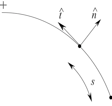
Consider a curved boundary, along which the values forψ and∂ψ/∂nare prescribed (Figure

2). It can be seen that the values of∂ψ/∂xand∂ψ/∂yon the boundary can then be obtained

in a straightforward manner. Let s be the arc length of the boundary. By introducing an

interpolating scheme (e.g. 1D-IRBFNs), one is able to derive derivatives of ∂ψ/∂x and

∂ψ/∂y with respect to s such as ∂2_{ψ/∂x∂sand ∂}2_ψ/∂y∂s.

following formula

∂f ∂s =

∂f ∂xtx+

∂f

∂yty, (14)

wheretx and ty are the two xand y components of the unit vectorbt tangential to the curve

(tx =∂x/∂sand ty =∂y/∂s).

Replacing f with ∂ψb/∂x, one has

∂2_ψ

b ∂x∂s =

∂2_ψ

b ∂x2 tx+

∂2_ψ

b

∂x∂yty, (15)

or

∂2_ψ

b ∂x∂y =

1 ty

∂2_ψ

b ∂x∂s−

∂2_ψ

b ∂x2 tx

, (16)

where ∂2_ψ

b/∂x∂sis considered as a known quantity.

Similarly, taking f as∂ψb/∂y results in

∂2_ψ

b ∂x∂y =

1 tx

∂2_ψ

b ∂y∂s−

∂2_ψ

b ∂y2 ty

, (17)

where ∂2_ψ

b/∂y∂sis a known value.

From (16) and (17), one can derive the relationship between ∂2_ψ/∂x2 _{and ∂}2_ψ/∂y2 _{at a}

boundary point

1 ty

∂2_ψ

b ∂x∂s −

∂2_ψ

b ∂x2 tx

= 1

tx

∂2_ψ

b ∂y∂s −

∂2_ψ

b ∂y2 ty

. (18)

Consider anxgrid line. The interpolating scheme employed along this line does not facilitate

the computation of second-order derivative of ψ with respect to they coordinate. However,

such a derivative at a boundary point can be found by using (18)

∂2_ψ

b ∂y2 =

tx ty

2

∂2_ψ

b

where qy is a known quantity defined by

qy =− tx t2

y ∂2_ψ

b ∂x∂s +

1 ty

∂2_ψ

b

∂y∂s. (20)

By substituting (19) into (13), a boundary condition for the vorticity at a boundary point

on a horizontal grid line will be computed by

ωb = " 1 + tx ty 2#

∂2_ψ

b

∂x2 +qy, (21)

where only the approximations in the x direction are needed.

In the same manner, on a vertical grid line, a boundary condition for the vorticity at a

boundary point will be computed by

ωb = " 1 + ty tx 2#

∂2_ψ

b

∂y2 +qx, (22)

where qx is a known quantity defined by

qx =− ty t2

x ∂2_ψ

b ∂y∂s +

1 tx

∂2_ψ

b

∂x∂s. (23)

The boundary conditions for the vorticity are thus written in terms of second derivative of

the stream function with respect to x or y only.

3.3

Numerical implementation of vorticity boundary conditions

As mentioned earlier, normal derivative boundary conditions for the stream function are used

for solving the transport vorticity equation. As a result, the values of ∂ψ/∂x and ∂ψ/∂y at

the boundary points have to be incorporated into (21) and (22), respectively.

It is well known that the computational vorticity boundary conditions strongly affect the

derivative using integrated RBFs only, the 1D-IRBFN scheme of at least second order needs

be employed. As shown in [20], higher-order IRBFNs can give more accurate results. In this

study, we attempt to employ 1D-IRBFNs of order 2 (Scheme 1) and 4 (Scheme 2), in which

second and fourth derivatives of ψ are respectively decomposed into RBFs, to evaluate

∂2_ψ/∂x2 _{and ∂}2_ψ/∂y2 _{in (21) and (22). A distinguishing feature here is that derivative}

boundary values, ∂ψ/∂x and ∂ψ/∂y, are incorporated into the IRBFN approximations by

means of the constants of integration.

Along an x grid line, the conversion process of the network-weight space into the physical

space can be described as follows

b

B

   wb

b c   =       b ψ b ψb c ∂ψb ∂x     

, (24)

wherebcis a vector of integration constants,wbandψbare defined as before,ψbb = (ψ(xb1), ψ(xb2))T,

d ∂ψb

∂x =

∂ψ(xb1)

∂x ,

∂ψ(xb2)

∂x T , and b B =    c B1 c B2   , in which c

B1 =Ib_[2](0),

c

B2 =

   I

(1)

1 (xb1) I2(1)(xb1) · · · Im(1)(xb1) 1 0

I₁(1)(xb2) I2(1)(xb2) · · · Im(1)(xb2) 1 0

for Scheme 1, and

c

B1 =Ib_[4](0) =

        

I₁(0)(x1) I2(0)(x1) · · · Im(0)(x1) x31/6 x21/2 x1 1

I₁(0)(x2) I2(0)(x2) · · · Im(0)(x2) x32/6 x22/2 x2 1

... ... . .. ... ... ... ... ... I₁(0)(xm) I2(0)(xm) · · · Im(0)(xm) x3m/6 x2m/2 xm 1

         , c

B2 =

   I

(1)

1 (xb1) I2(1)(xb1) · · · Im(1)(xb1) x2b1/2 xb1 1 0

I₁(1)(xb2) I2(1)(xb2) · · · Im(1)(xb2) x2b2/2 xb2 1 0

  ,

for Scheme 2, where I_i(4)(x) =gi(x),Ii(3)(x) = R

I_i(4)(x), _{· · ·}, I_i(0)(x) =R I_i(1)(x).

Taking (24) into account, second derivatives ofψat the two boundary points can be expressed

in terms of the values of ψ at every point on the grid line and the values of ∂ψ/∂x at the

two boundary points

d ∂2_ψ

b

∂x2 =DbBb

−1       b ψ b ψb c ∂ψb ∂x     

, (25)

where

b

D =  

 g1(xb1) g2(xb1) · · · gm(xb1) 0 0 g1(xb2) g2(xb2) · · · gm(xb2) 0 0

  

for Scheme 1, and

b D =    I (2)

1 (xb1) I2(2)(xb1) · · · Im(2)(xb1) xb1 1 0 0

I₁(2)(xb2) I2(2)(xb2) · · · Im(2)(xb2) xb2 1 0 0

  

for Scheme 2.

It should be emphasised that the IRBFN approximation for∂2_ψ/∂x2 _{satisfies normal}

deriva-tive of ψ at the two boundary points identically. Substituting (25) into (21), one is able to

obtain the boundary conditions for the vorticity equation.

line is similar to that on a horizontal line.

3.4

Solution procedure

The three governing equations must be solved simultaneously to find the values of the

tem-perature, vorticity and stream function at the discrete points within the domain. In this

paper, a time marching approach is adopted and at each time step, to minimise the memory

requirement, the three equations are solved in a sequential manner. The solution procedure

involves the following main steps.

1. Guess the distributions of T, ω and ψ.

2. Discretise the governing equations in time using a first-order accurate finite-difference

scheme, where the diffusive and convective terms are treated implicitly and explicitly,

respectively.

3. Discretise the governing equations in space using 1D-IRBFNs. Since the differentiation

matrices are the same for all variables, the construction process only needs to be carried

out for one variable. The system matrices, which involve the IRBFN approximations for

the Laplacian operator in the governing equations, stay the same during the iteration

process. All equations are subject to Dirichlet boundary conditions.

4. Solve the energy equation (3) for T.

5. Derive computational boundary conditions for ω.

6. Solve the vorticity equation (1) for ω.

vergence measure (CM)

CM = r

Pnip

i=1

ψi(k)−ψ

(k−1)

i 2

r Pnip

i=1

ψ(_ik)2

< ǫ, (26)

wherenip is the number of interior points,k the time level and ǫ the tolerance (in this

study, ǫ is taken to be 10−12).

9. If it is not satisfied, advance time step and repeat from step 4. Otherwise, stop the

computation and output the results.

4

Numerical examples

The first two examples, for which analytic solutions are available, are used to verify the

vorticity boundary formula and its numerical implementations on both simply- and

multiply-connected domains. In the last two examples, the proposed technique is applied for the

simulation of natural convection in the region between two concentric cylinders. The thermal

boundary conditions are prescribed asT = 0 andT = 1 along the stationary outer and inner

walls, respectively.

The present technique implements the multiquadric (MQ) basis function whose form is

gi(x) = q

(x₋ci)2+a2i, (27)

where ci and ai are the centre and the width of the ith MQ function.

For all numerical examples presented in this study, the problem domain is discretised with

a uniform Cartesian grid. The width of theith MQ-RBF, ai, is simply chosen to be the grid

spacingh(grid size), and the interior points that fall very close to the boundary (within the

distance of h/8) are removed from the set of nodal points. In the first two examples, the

defined as

N e=

qPM

i=1(fie−fi)2 qPM

i=1(fie)2

, (28)

where M is the number of unknown nodal values of f, and fe _{and f are the exact and}

approximate solutions, respectively. Another important measure is the convergence rate of

the solution with respect to the refinement of spatial discretisation

N e(h)_≈γhα =O(hα), (29)

in which α and γ are exponential model’s parameters. Given a set of observations, these

parameters can be found by the general linear least squares technique.

4.1

Example 1: Circular shape domain

The present technique is first verified through the solution of the following test problem

governed by

∂2_ψ

∂x2 +

∂2_ψ

∂y2 =ω, (30)

∂2_ω

∂x2 +

∂2_ω

∂y2 =b(x, y), (31)

on a unit circular domain with the boundary conditions in terms ofψ and∂ψ/∂n. The exact

solution of this problem is taken as

ψe= cos( p

x2_+y2_{), (32)}

analyt-the present domain are simply computed by

tx = − y p

x2_+y2, (33)

ty = x p

x2_+y2. (34)

Expressions for the vorticity at the boundary nodes on thex and ygrid lines thus reduce to

ωb =

1 +y x

2_∂2_ψb

∂x2 +qy, (35)

ωb = "

1 +

x y

2#

∂2_ψ

b

∂y2 +qx, (36)

each of which only requires the approximation of second-order derivative of ψ with respect

to one coordinate direction. Both Scheme 1 and Scheme 2 are employed to compute the

above expressions.

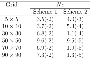
We conduct two investigations here: (i) the accuracy of Scheme 1 and Scheme 2 for

approx-imating∂2_ψ/∂x2 _{in (35), and (ii) the accuracy of the RBF solution to the PDEs.}

For the former, calculations are carried out for various grids from 5_×5 to 90_×90. Results

of N e obtained by the two different order interpolating schemes are displayed in Table 1,

which show that Scheme 2 gives much more accurate results than Scheme 1. Scheme 2 is

thus recommended for use in practice.

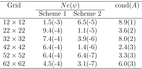
For the latter, a number of grids, namely (12_×12,22_×22,_{· · ·} ,62_×62), are employed to

study the convergence behaviour of the solution. Results concerning the condition number of

the system matrix, denoted by cond(A), and the errorN eare given in Table 2. The present

technique produces system matrices with relatively-low condition numbers. For example,

the matrix condition number is only 6.0_×103 _{for a grid of 62×62. It can be seen that}

the choice of Scheme 1 (1D-IRBFN-2s) and Scheme 2 (1D-IRBFN-4s) for computing ωb in

(35) and (36) has a profound influence on the overall accuracy of the IRBFN solution. The

fourth-order boundary scheme outperforms the second-order one regarding both accuracy

4.2

Example 2: Multiply-connected domain

This test problem is also governed by the two coupled equations (30) and (31) with Dirichlet

boundary conditions, ψ and ∂ψ/∂n. The driving function is taken as

b(x, y) = 256(π2₋1)2[sin(4πx) cosh(4y) + cos(4πx) sinh(4y)], (37)

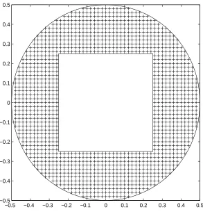
and the domain of interest is the region lying between a circle of radius 1/2 and a square of

dimensions 1/2_×1/2 which are both centered at the origin (Figure 4). The exact solution

for this problem is

ψe= sin(4πx) cosh(4y)−cos(4πx) sinh(4y). (38)

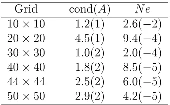
A number of uniform grids, (10 _× 10,20 _× 20, ...,50 _× 50), are considered. Since inner

boundaries are parallel to the x and y axes, one can use the original formula for deriving a

computational vorticity boundary condition. The stream-function equation can be rewritten

as

ωb = ∂2_ψ

b ∂n2 +

∂2_ψ

b

∂t2 , (39)

where ∂2_ψ

b/∂t2 is a known quantity derived from the boundary conditions for ψ, and ∂2_ψ

b/∂n2 can be evaluated using a grid line passing through that point. On the outer

boundary, the handling of ωb is similar to that in the previous example. For brevity, only

the recommended scheme (i.e. Scheme 2) for computing ωb is employed here. Results

con-cerningN e(ψ) are given in Table 3, from which one can also make remarks that are similar

to those in the case of simply-connected domains. It can be seen that the present matrix

condition numbers are relatively low and the approximate solution converges fast to the

exact solution with a rate ofO(h3.78_).

heated (T = 1) and the outer cylinder cooled (T = 0) (Figure 5a). A comprehensive review

of this problem can be found in [2]. Most cases have been reported with P r = 0.7 and

L/Di = 0.8, in which Di is the diameter of the inner cylinder. To these conditions, results

by Kuehn and Goldstein [2] using FDM for Ra = 102 _{to Ra = 7× 10}4 _{are often cited}

in the literature for comparison purposes. Later on, Shu [11], who employed a differential

quadrature method (DQM), has provided very accurate solutions for the values ofRain the

range of 102 _{to 5×10}4_{. It is noted that those works required a computational domain be}

rectangular.

The three governing equations (1), (2), (3) are presently solved with respective to Cartesian

coordinates (Figure 5a). Numerical simulations are also conducted forP r= 0.7 andL/Di =

0.8. Like in the case of [2], we consider the values of the Rayleigh number from Ra = 102

to Ra = 7_× 104_{, which is broader than those reported in [11]. Different grids, namely}

(12_×12,22_×22,_{· · ·} ,52_×52), are employed.

The stream function and its normal derivative are set to zero along the inner and outer

cylinders. Expressions (35) and (36) derived in Example 1 are applicable here to compute

the values of the vorticity on the cylinder walls. Since the boundary values for ∂ψ/∂x and

∂ψ/∂y are simply zeros, the terms qx and qy vanish. The values for the vorticity at the

boundary nodes on the x and y grid lines can thus be computed by

ωb = [1 + ( y x)

2_]∂2ψb

∂x2 , (40)

ωb = [1 + ( x y)

2_]∂2ψb

∂y2 , (41)

respectively. As mentioned earlier, Neumann boundary conditions for the stream function,

∂ψ/∂x = 0 and ∂ψ/∂x = 0, are presently incorporated into the computational vorticity

boundary conditions via integration constants and they are satisfied identically.

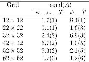
Table 4 indicates a significant improvement in the matrix condition number of the present

formulation over the stream function-temperature formulation reported in [19]. The former

feature is very attractive in the context of RBF techniques. One is thus able to use a larger

number of nodes with the present approach in the RBF simulation of fluid flow problems.

Both accuracy and grid convergence of the present technique are investigated.

The solution accuracy is assessed through the average equivalent conductivity defined as

(e.g. [2, 11])

¯

keq = −

ln(Do/Di)

2π

I ∂T

∂nds, (42)

in which Do and Di are the diameters of the outer cylinder and the inner cylinder,

respec-tively. Results concerning ¯keq together with those of Kuehn and Goldstein [2] and of Shu

[11] forRa=_{102_,103_,3×103_,6×103_,104_,5×104_,7×104_{}are presented in Table 5. It can}

be seen that there is a good agreement between these numerical solutions.

Figures 6 and 7 show the convergence of the stream function and temperature fields with

respect to grid refinement for Ra = 104 _{and Ra = 7×10}4_{, respectively. It can be seen}

that the present technique is able to capture complex structures of the stream function

and temperature fields even at coarse grids, and those patterns are improved in quality

(smoothness) with increasing grid-densities. At a grid of 42_×42 for Ra= 104 _{and a grid of}

52_×52 for Ra= 7_×104_{, the plots look reasonable when compared with those reported in}

[2, 11].

4.4

Example 4: Concentric annulus between a square outer

cylin-der and a circular inner cylincylin-der

For this example, natural convection between a heated inner circular cylinder and a cooled

square enclosure is considered (Figure 5b). It is noted that the transformation of this domain

of the inner circle), P r = 0.71 and Ra= _{104_,5×104_,105_,5×105_,106_{} are employed here}

to investigate the accuracy of the technique.

An attractive feature here is that the present technique does not require any coordinate

transformations. The problem domain is simply replaced with a Cartesian grid (Figure 5b).

Numerical results are obtained for three uniform grids of 32_×32, 42_×42, and 52_×52.

For Ra = 104_{, we start to simulate the flow from rest. For higher values of Ra, the initial}

solution is taken as the solution obtained at lower and nearest Ra. Figure 8 presents the

behaviour of the convergence measure CM against the number of time steps. It can be seen

that the decrease inCM is rather monotonic. As expected, the simulation of high-Raflows

requires a larger number of iterations.

The obtained results are presented in Table 6 and Figure 9. Table 6 is concerned with the

accuracy of the solution. Following the work of Moukalled and Acharya [12], the local heat

transfer coefficient is defined as

h=₋k∂T

∂n, (43)

where k is the thermal conductivity. The average Nusselt number (the ratio of the

temper-ature gradient at the wall to a reference tempertemper-ature gradient) is computed by

N u= h

k, (44)

whereh=₋H ∂T

∂nds. Since the computational domain in [12] is taken as one-half of the

phys-ical domain, the values ofN uin the present work (Table 6) are divided by 2 for comparison

purposes. The present results agree well with those in [12] and [13].

Figure 9 displays streamlines and isotherms versus grid densities for Ra= 106_{, which shows}

a very fast convergence of all fields. The qualitative behaviour of these fields and those in

5

Concluding remarks

In this article, a new numerical discretisation scheme for the stream function vorticity

-temperature formulation using Cartesian grids and 1D-IRBFNs is reported. Attractive

fea-tures of the proposed technique include (i) the preprocessing is simple and (ii) the boundary

conditions for the vorticity are implemented in a new and effective manner. Numerical results

show that (i) the matrix condition number is significantly improved over the stream

func-tion - temperature formulafunc-tion and (ii) accurate results are obtained using a relatively-coarse

grid.

Acknowledgements

This research is supported by the Australian Research Council. K. Le-Cao wishes to thank

the CESRC, FoES and USQ for a postgraduate scholarship.

References

[1] G. de Vahl Davis, Natural convection of air in a square cavity: a bench mark numerical

solution, Int. J. for Numerical Methods in Fluids, vol. 3, pp. 249-264, 1983.

[2] T.H. Kuehn, and R.J. Goldstein, An experimental and theoretical study of natural

con-vection in the annulus between horizontal concentric cylinders, J. of Fluid Mechanics,

vol. 74(4), pp. 695-719, 1976.

[3] M.T. Manzari, An explicit finite element algorithm for convection heat transfer problems,

Int. J. of Numerical Methods for Heat and Fluid Flow, vol. 9(8), pp. 860-877, 1999.

[4] H. Sammouda, A. Belghith, C. Surry, Finite element simulation of transient natural

[5] E.K. Glakpe, C.B. Watkins, and J.N. Cannon, Constant heat flux solutions for

natu-ral convection between concentric and eccentric horizontal cylinders, Numerical Heat

Transfer - Part B, vol. 10, pp. 279-295, 1986.

[6] D.A. Kaminski, and C. Prakash, Conjugate natural convection in a square enclosure:

effect of conduction in one of the vertical walls, Int. J. for Heat and Mass Transfer, vol.

29(12), pp. 1979-1988, 1986.

[7] M. Hribersek, and L. Skerget, Fast boundary-domain integral algorithm for the

compu-tation of incompressible fluid flow problems, Int. J. for Numerical Methods in Fluids,

vol. 31, pp. 891-907, 1999.

[8] K. Kitagawa, L.C. Wrobel, C.A. Brebbia, and M. Tanaka, A boundary element

formu-lation for natural convection problems, Int. J. for Numerical Methods in Fluids, vol. 8,

pp. 139-149, 1988.

[9] G. Kosec, and B. Sarler, Solution of thermo-fluid problems by collocation with local

pressure correction, Int. J. of Numerical Methods for Heat & Fluid Flow, vol. 18 (7/8),

pp. 868-882, 2008.

[10] P. Le Quere, Accurate solutions to the square thermally driven cavity at high Rayleigh

number, Computers & Fluids, vol. 20(1), pp. 29-41, 1991.

[11] C. Shu, Application of differential quadrature method to simulate natural convection in

a concentric annulus, Int. J. for Numerical Methods in Fluids, vol. 30, pp. 977-993, 1999.

[12] F. Moukalled, and S. Acharya, Natural convection in the annulus between concentric

horizontal circular and square cylinders, J. of Thermophysics and Heat Transfer, vol.

10(3), pp. 524-531, 1996.

[13] C. Shu, and Y.D. Zhu, Efficient computation of natural convection in a concentric

annulus between an outer square cylinder and an inner circular cylinder, Int. J. for

Numerical Methods in Fluids, vol. 38, pp. 429-445, 2002.

[14] G.E. Fasshauer, Solving partial differential equations by collocation with radial basis

Rabut, and L.L. Schumaker), pp. 131-138, Vanderbilt University Press, Nashville, TN,

1997.

[15] E.J. Kansa, Multiquadrics- A scattered data approximation scheme with applications to

computational fluid-dynamics-II. Solutions to parabolic, hyperbolic and elliptic partial

differential equations, Computers and Mathematics with Applications, vol. 19(8/9), pp.

147-161, 1990.

[16] N. Mai-Duy, and T. Tran-Cong, Approximation of function and its derivatives using

radial basis function networks, Applied Mathematical Modelling, vol. 27, pp. 197-220,

2003.

[17] B. Sarler, A radial basis function collocation approach in computational fluid dynamics,

Computer Modeling in Engineering & Sciences, vol. 7(2), pp. 185-194, 2005.

[18] N. Mai-Duy, and T. Tran-Cong, A Cartesian-grid collocation method based on

radial-basis-function networks for solving PDEs in irregular domains, Numerical Methods for

Partial Differential Equations, vol. 23(5), pp. 1192-1210, 2007.

[19] N. Mai-Duy, K. Le-Cao, and T. Tran-Cong, A Cartesian grid technique based on

one-dimensional integrated radial basis function networks for natural convection in

conccen-tric annuli, Int. J for Numerical Methods in fluids, vol. 57, pp. 1709-1730, 2008.

[20] N. Mai-Duy, Solving high order ordinary differential equations with radial basis function

networks, Int. J. for Numerical Methods in Engineering, vol. 62, pp. 824-852, 2005.

[21] S. Ostrach, Natural convection in enclosures, J. of Heat Transfer, vol. 110, pp.

Grid N e

Scheme 1 Scheme 2 5_×5 3.5(-2) 4.0(-3) 10_×10 3.7(-2) 5.3(-4) 30_×30 6.8(-2) 1.1(-4) 50_×50 9.6(-2) 9.5(-5) 70_×70 6.9(-2) 1.9(-5) 90_×90 7.3(-2) 1.3(-5)

Grid N e(ψ) cond(A) Scheme 1 Scheme 2

12_×12 1.5(-3) 6.5(-5) 8.9(1) 22_×22 9.4(-4) 1.1(-5) 3.6(2) 32_×32 7.4(-4) 3.9(-6) 8.0(2) 42_×42 6.4(-4) 1.4(-6) 2.4(3) 52_×52 6.4(-4) 6.4(-7) 3.3(3) 62_×62 4.5(-4) 3.1(-7) 6.0(3)

Grid cond(A) N e 10_×10 1.2(1) 2.6(₋2) 20_×20 4.5(1) 9.4(₋4) 30_×30 1.0(2) 2.0(₋4) 40_×40 1.8(2) 8.5(₋5) 44_×44 2.5(2) 6.0(₋5) 50_×50 2.9(2) 4.2(₋5)

Table 3: Example 2: Condition numbers of the system matrix and relative L2 errors of the

Grid cond(A) ψ₋ω₋T ψ₋T 12_×12 1.7(1) 8.4(1) 22_×22 9.1(1) 1.6(3) 32_×32 2.4(2) 6.9(3) 42_×42 6.7(2) 1.0(5) 52_×52 9.3(2) 2.1(5) 62_×62 1.7(3) 1.2(6)

Ra 102 ₁₀3 _3×103 _6×103 ₁₀4 _5×104 _7×104

keqi

Present Method 1.000 1.083 1.396 1.709 1.975 2.962 3.207 FDM [2] 1.000 1.081 1.404 1.736 2.010 3.024 3.308 DQM [11] 1.001 1.082 1.397 1.715 1.979 2.958

keqo

Present Method 0.999 1.080 1.393 1.712 1.970 2.942 3.246 FDM [2] 1.002 1.084 1.402 1.735 2.005 2.973 3.226 DQM [11] 1.001 1.082 1.397 1.715 1.979 2.958

Table 5: Example 3 (circular cylinders): Comparison of the average equivalent conductivity on the outer and inner cylinders,keqi and keqo, between the present IRBFN technique using

Ra 104 _5×104 ₁₀5 _5×105 ₁₀6

N uo

Present Method 3.22 4.04 4.89 7.43 8.70 FDM [12] 3.24 4.86 8.90 DQM [13] 3.33 5.08 9.37

N ui

Present Method 3.21 4.04 4.89 7.51 8.85 FDM [12] 3.24 4.86 8.90 DQM [13] 3.33 5.08 9.37

Table 6: Example 4 (square-circular cylinders): Comparison of the average Nusselt number on the outer and inner cylinders, N uo and N ui, forRa from 104 to 106 between the present

x1 x2 xq

xb1 xb2

−1 −0.8 −0.6 −0.4 −0.2 0 0.2 0.4 0.6 0.8 1 −1

−0.8 −0.6 −0.4 −0.2 0 0.2 0.4 0.6 0.8 1

−0.5 −0.4 −0.3 −0.2 −0.1 0 0.1 0.2 0.3 0.4 0.5 −0.5

−0.4 −0.3 −0.2 −0.1 0 0.1 0.2 0.3 0.4 0.5

(a) (b)

22_×22

32_×32

42_×42

Figure 6: Circular-circular cylinders: Convergence of the temperature (left) and stream function (right) fields with respect to grid refinement for the flow at Ra = 104_{. Each plot}

32_×32

42_×42

52_×52

Figure 7: Circular-circular cylinders: Convergence of the temperature (left) and stream function (right) fields with respect to grid refinement for the flow atRa= 7_×104_{. Each plot}

0 2000 4000 6000 8000 10000 12000 14000 16000 18000 −14

−12 −10 −8 −6 −4 −2 0

Number of iterations

lo

g

(

N

e

)

Figure 8: Iterative convergence. Time steps used are 0.002 for Ra = 104_{, 0.005 for Ra =}

5_×104_{, and 0.008 for Ra = {10}5_,5×105_,106_{}. The values of CM become less than 10}−12

when the numbers of iterations reach 10925, 9740, 8609, 15017, and 17938 forRa=_{104_,5×

32_×32

42_×42

52_×52