University of Southern Queensland
Faculty of Engineering & Surveying
Investigation of TCP Performance Over
Wireless Internet.
A dissertation submitted by
Peh Wee Liang
in fulfilment of the requirements of
ENG 4112 Research Project
towards the degree of
Bachelor of Electrical and Electronic Engineering
Abstract
The demand for providing Internet services over wireless links has grown rapidly in recent years. Although TCP (Transmission Control Protocol) has been performing well
over the traditional wired networks where packet losses occur mostly because of congestion, it cannot react efficiently in wireless networks, which suffer from significant non-congestion-related losses due to reasons such as bit errors and handoffs.
The main reason for this poor performance of TCP is the fact that it cannot distinguish between packet losses due to wireless errors from those due to congestion. It responds to all losses by invoking congestion control and avoidance algorithms. Moreover, TCP sender cannot keep the size of its congestion window at optimum level and always has to retransmit packets after waiting for timeout, which significantly degrades end-to-end delay performance of TCP.
University of Southern Queensland
Faculty of Engineering and Surveying
ENG4111 & ENG4112 Research Project
Limitations of Use
The Council of the University of Southern Queensland, its Faculty of Engineering and Surveying, and the staff of the University of Southern Queensland, do not accept any responsibility for the truth, accuracy or completeness of material contained within or associated with this dissertation.
Persons using all or any part of this material do so at their own risk, and not at the risk of the Council of the University of Southern Queensland, its Faculty of Engineering and Surveying or the staff of the University of Southern Queensland.
This dissertation reports an educational exercise and has no purpose or validity beyond this exercise. The sole purpose of the course pair entitled "Research Project" is to contribute to the overall education within the student’s chosen degree program. This document, the associated hardware, software, drawings, and other material set out in the associated appendices should not be used for any other purpose: if they are so used, it is entirely at the risk of the user.
Prof G Baker
Dean
Certification of Dissertation
I certify that the ideas, designs and experimental work, results, analysis and conclusion set out in this dissertation are entirely my own effort, except where otherwise indicated
and acknowledged.
I further certify that the work is original and has not been previously submitted for assessment in any other course or institution, except where specifically stated.
Peh Wee Liang
D11338609
_____________________ Signature
Acknowledgments
I would like to express my gratitude toward Dr. Hong Zhou and Dr. John Leis for their constant information, suggestions and guidance. I am grateful for the opportunity of
working under them on such an interesting Undergraduate Research project.
My thanks is also extended to friends and classmates, who had advise and seen me through the difficulties I had encountered throughout the course of the project.
Most importantly I would like to thank my family whose constant support, kind patience and understanding I could not do without.
Peh Wee Liang
University of Southern Queensland
Contents
Abstract i
Acknowledgments iv
List of Figures viii
Chapter 1 Introduction 1
1.1 Project Background ... 1
1.2 Project Aims ... 2
1.3 Specific Objectives ... 3
Chapter 2 Transmission Control Protocol (TCP) 4 2.1 Introduction ... 4
2.2 Flow Control... 6
2.3 Congestion Control... 10
2.3.1 Slow Start ... 10
2.3.2 Congestion Avoidance... 12
CONTENTS vi
2.4 TCP in Wireless Link ... 16
Chapter 3 Snoop Protocol 18 3.1 Introduction ... 18
3.2 Algorithms ... 20
3.3 Performance Analysis... 24
3.4 Advantages and Disadvantages ... 29
Chapter 4 Explicit Loss Notification (ELN) 32 4.1 Introduction ... 32
4.2 Algorithms ... 35
4.3 Performance Analysis... 43
4.4 Advantages and Disadvantages ... 50
Chapter 5 Explicit Congestion Notification (ECN) 52 5.1 Introduction ... 52
5.2 Algorithms ... 54
5.3 Performance Analysis... 59
CONTENTS vii
Chapter 6 Simulation Methodology 67
6.1 Selection of Simulation Tools ... 67
6.2 Introduction to Network Simulator 2 (NS2)... 70
6.2.1 Features... 71
6.2.2 Network Animator (NAM)... 74
6.2.3 Basic Command... 76
Chapter 7 Installation of Linux and Network Simulator 2 (NS2) 82 7.1 Red Hat Linux Installation Process ... 82
7.2 Network Simulator 2 Installation Process ... 98
Chapter 8 Conclusions and Further Work 101 8.1 Conclusions ... 101
8.2 Further Work ... 104
References 107
List of Figures
Figure 2.1: Receiver Buffer ... 6
Figure 2.2: Flow Control part 1 ... 7
Figure 2.3: Flow Control part 2 ... 8
Figure 2.4: Flow Control part 3 ... 9
Figure 2.5: TCP transmission window... 11
Figure 2.6: Fast Retransmit part 1... 13
Figure 2.7: Fast Retransmit part 2... 14
Figure 2.8: Fast Retransmit part 3... 15
Figure 2.9: Wireless link using TCP... 16
Figure 3.1: Adding the Snoop agent. ... 18
Figure 3.2: Snoop Protocol part 1 ... 20
Figure 3.3: Snoop Protocol part 2 ... 21
LIST OF FIGURES ix
Figure 3.5: Snoop Protocol part 4 ... 23
Figure 3.6: Snoop Protocol test bed setup 1 ... 24
Figure 3.7: Variable delay between BS and MH ... 25
Figure 3.8: Variable delay between BS and FH ... 25
Figure 3.9: Snoop performance with different corruption rates ... 26
Figure 3.10: Snoop Protocol test bed setup 2 ... 27
Figure 3.11: Throughput received by the mobile host at different bit-error rates ... 28
Figure 3.12: Performance on a Web workload in different protocol configurations.... 30
Figure 4.1: ELN part 1 ... 35
Figure 4.2: ELN part 2 ... 36
Figure 4.3: ELN part 3 ... 37
Figure 4.4: ELN part 4 ... 38
Figure 4.5: ELN part 5 ... 39
Figure 4.6: ELN part 6 ... 40
Figure 4.7: ELN part 7 ... 41
Figure 4.8: ELN part 8 ... 42
Figure 4.9: ELN test bed setup ... 43
Figure 4.10: Throughput performance comparison ... 44
Figure 4.11: End-to-end delay for TCP-Reno (without wireless error)... 45
Figure 4.12: End-to-end delay for TCP-Reno (wireless packet loss rate = 0.1)... 46
LIST OF FIGURES x
Figure 4.14: Window evolution for TCP-Reno (wireless packet loss rate = 0.1)... 48
Figure 4.15: Window evolution for ELN-ACK (wireless packet loss rate = 0.1) ... 48
Figure 4.16: Throughput of TCP Reno and Reno enhanced with ELN... 50
Figure 5.1: ECN part 1... 54
Figure 5.2: ECN part 2... 55
Figure 5.3: ECN part 3... 56
Figure 5.4: ECN part 4... 57
Figure 5.5: ECN part 5... 58
Figure 5.6: ECN test bed setup 1 ... 59
Figure 5.7: RED and ECN Goodput ... 60
Figure 5.8: Goodput with 30 flows ... 60
Figure 5.9: Goodput with 120 flows ... 61
Figure 5.10: ECN test bed setup 2 ... 62
Figure 5.11. Total number of packets sent by the FTP server to all ten clients... 63
Figure 5.12: Total number of packets sent by the FTP server to all ten clients (with longer delays)... 63
Figure 6.1: Trace Format Example ... 71
Figure 6.2: X Graph ... 73
Figure 6.3: NAM display ... 74
Figure 6.4: NAM display for a simple communication scenario... 75
LIST OF FIGURES xi
Figure 7.1: Red Hat installation process (Boot Prompt)... 83
Figure 7.2: Red Hat installation process (Anaconda) ... 84
Figure 7.3: Red Hat installation process (Language Selection)... 84
Figure 7.4: Red Hat installation process (Keyboard Configuration) ... 85
Figure 7.5: Red Hat installation process (Mouse Configuration) ... 85
Figure 7.6: Red Hat installation process (Welcome to Red Hat Linux) ... 86
Figure 7.7: Red Hat installation process (Install Options)... 86
Figure 7.8: Red Hat installation process (Partition part 1) ... 87
Figure 7.9: Red Hat installation process (Partition part 2) ... 87
Figure 7.10: Red Hat installation process (Partition part 3) ... 88
Figure 7.11: Red Hat installation process (Partition part 4) ... 88
Figure 7.12: Red Hat installation process (Boot Loader Installation) ... 89
Figure 7.13: Red Hat installation process (GRUB Password)... 89
Figure 7.14: Red Hat installation process (Network Configuration)... 90
Figure 7.15: Red Hat installation process (Firewall Configuration)... 90
Figure 7.16: Red Hat installation process (Language Support Selection) ... 91
Figure 7.17: Red Hat installation process (Time Zone Selection)... 91
Figure 7.18: Red Hat installation process (Account Configuration) ... 92
Figure 7.19: Red Hat installation process (Selecting Package Group) ... 92
Figure 7.20: Red Hat installation process (Video Configuration) ... 93
Figure 7.21: Red Hat installation process (Installing Package part 1)... 93
LIST OF FIGURES xii
Figure 7.23: Red Hat installation process (Installing Package part 3)... 94
Figure 7.24: Red Hat installation process (Boot Disk Creation) ... 95
Figure 7.25: Red Hat installation process (Monitor Selection) ... 95
Figure 7.26: Red Hat installation process (X Configuration) ... 96
Figure 7.27: Red Hat installation process (Congratulations-Linux has been installed) 96 Figure 7.28: Red Hat installation process (Graphical Boot Loader Prompt)... 97
Figure 8.1: Network topology 1... 105
Chapter 1
Introduction
1.1 Project Background
The term wireless refers to telecommunication technology in which radio waves such as infrared waves and microwaves are used to carry a signal to connect communication devices, instead of cables or wires. These devices include pagers, cell phones, portable
PCs, computer networks, location devices, satellite systems and handheld digital assistants. Wireless technology is rapidly evolving, and is fast becoming an important role in the lives of people around the world. Wireless technology enables users to physically move while using an appliance, such as a handheld PC, paging device, or phone. Without the physical connection of cables or wires, this technology allows users to check stocks and email from their internet-enabled devices.
Chapter 1: Project Aims 2
way of a connection, a wireless solution may be more economical than installing physical cable. Wires and connectors can easily break through misuse and normal wear
and tear. Therefore using less cable reduces the downtime of the network and the costs associated with replacing cables, and makes the network available for use much sooner. http://wireless.ittoolbox.com/pub/wireless_overview.htm (2002)
Pilosof et al. (2002) noted that the result of the growth in usage of wireless networking, has caused the focus to turn to deploying wireless Internet over hot spots such as airports, hotels, cafes, and other areas from which people can have uninterrupted public access to the Internet. As these networks see increasing public deployment, it is important for the service providers to be able to ensure that access to the network by different users and applications remains impartial. Since the majority of today’s applications in Internet use Transmission Control Protocol (TCP), this project will focus on the performance of TCP in wireless Internet.
1.2 Project Aims
Chapter 1: Specific Objectives 3
1.3 Specific Objectives
This research will investigate the performance of a few representative mechanisms, that is, Snoop protocol, Explicit Loss Notification (ELN), Explicit Congestion Notification (ECN). This project also aims to:
• Study protocols and representative mechanisms: TCP/IP, Snoop protocol, Explicit Loss Notification (ELN) and Explicit Congestion Notification (ECN). • Compare the performance with regular TCP with the representative
mechanisms.
Chapter 2
Transmission Control Protocol
(TCP)
2.1 Introduction
Transmission Control Protocol (TCP) is the most widely used transport layer protocol in
the Internet. Most popular Internet applications, such as the Web and file transfer, use the reliable services provided by TCP. Hassan and Jain (2001) noted that the performance perceived by users of these Internet applications depends largely on the performance of TCP.
In the Internet protocol suite, Internet Protocol (IP) is a best-effort service and TCP is a reliable service. IP provides the basic packet forwarding while TCP implements the flow controls, acknowledgements and retransmissions of lost or corrupted packets. This split in services "decentralizes" the network and moves the responsibility for reliable delivery to end systems. TCP is an end-to-end transport protocol, meaning that it runs in end systems, not the network. IP is a network protocol.
Chapter 2: Introduction 5
TCP is made reliable via the use of sequence numbers and acknowledgments. Conceptually, each octet of data is assigned a sequence number. The sequence number
of the first octet of data in a segment is transmitted with that segment and is called the segment sequence number. Segments also carry an acknowledgment number, which is the sequence number of the next expected data octet of transmissions in the reverse direction. When the TCP transmits a segment containing data, it puts a copy on a retransmission queue and starts a timer; when the acknowledgment for that data is received, the segment is deleted from the queue. If the acknowledgment is not received before the timer runs out, the segment is retransmitted. An acknowledgment by TCP does not guarantee that the data has been delivered to the end user, but only that the receiving TCP has taken the responsibility to do so. To govern the flow of data between TCP, a flow control mechanism is employed. http://www.ietf.org/rfc/rfc0793.txt (1981)
As noted by Biswas (2003), TCP is almost globally accepted as the standard for end-to-end reliable communication protocol. Therefore it is not feasible at any time to make changes to the core of TCP protocol, and expect the globe community to move over to the new version. Hence, efforts are being made to work around the shortcoming of TCP by hiding the underlying inconsistencies of the wireless link from the protocol. Some of the solutions that have been proposed are the Snoop Protocol, ELN and ECN, which increase TCP’s performance by hiding the packet losses over the wireless link.
Chapter 2: Flow Control 6
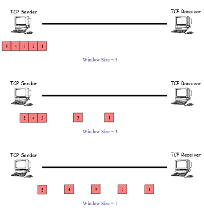
2.2 Flow Control
Flow-control mechanisms control packet flow so that a sender does not transmit more packets than a receiver can process. Flow controls are necessary because senders and receivers are often unmatched in capacity and processing power. A receiver might not be able to process packets at the same speed as the sender. If buffers fill, packets are dropped. The goal of flow-control mechanisms is to prevent the dropping of packets that must be retransmitted.
RevWindow
free space TCP data
RecBuffer
Figure 2.1: Receiver Buffer
Chapter 2: Flow Control 7
TCP Receiver TCP Sender
3 4 2
5 1
Window Size = 5
TCP Receiver TCP Sender
3 4
5 2 1
Window Size = 3
TCP Receiver TCP Sender
4 3 2 1
5
[image:20.612.120.532.86.522.2]Window Size = 1
Figure 2.2: Flow Control part 1
With reference to Figure 2.2, the initial receiver’s advertise window size is five. Thus
Chapter 2: Flow Control 8
TCP Receiver TCP Sender
5 4 3 2 1
Window Size = 0
TCP Sender TCP Receiver
ACK1
5 4 3 2 1
Window Size = 0
TCP Receiver TCP Sender
ACK2
ACK1
5 4 3 2 1
Window Size = 0
Figure 2.3: Flow Control part 2
As shown in Figure 2.3, after five packets are being transmitted by the sender, the
advertise window size will be zero, thus telling the sender to stop sending any data. The receiver will indicate its current window size to the sender by sending an acknowledgement (ACK) for every packet it received. In ACK1, the receiver has
advertised a window size of one. The reason why the sender is still not transmitting any data at the moment is because ACK1 has not reach the sender. Therefore the sender can
Chapter 2: Flow Control 9
TCP Sender TCP Receiver
ACK4
ACK2 ACK3
3 2
4 1
5
Window Size = 1
TCP Receiver TCP Sender
ACK5
ACK4
5 4 3 2 1
Window Size = 3
TCP Receiver TCP Sender
5 4 3 2 1
Window Size = 5
Figure 2.4: Flow Control part 3
In Figure 2.4, when ACK1 reaches the sender, the window size is increased to one. This
Chapter 2: Congestion Control 10
2.3 Congestion Control
Congestion control mechanisms allow network systems to detect network congestion (a condition in which there is more traffic on the network than can be handled by the network or network devices) and throttle back their transmission to alleviate the congestion. Congestion occurs on busy networks. When it occurs, end systems and the network must work together to minimize the congestion. In contrast, flow controls are used between end systems. A receiver uses flow controls to signal to the sender that it is overloaded. The sender then throttles back or stops its transmission.
http://www.linktionary.com/f/flow_control.html (2001)
Without congestion control, the receiver may indicate a large window, which encourages transmissions. However if more data packets arrive than can be accepted, it will be discarded. This will result in excessive retransmissions, adding unnecessarily to
the load on the network and the TCP. Indicating a small window may restrict the transmission of data to the point of under-utilizing the available bandwidth on the link. http://www.ietf.org/rfc/rfc0793.txt (1981)
2.3.1 Slow
Start
Slow Start mechanism is a feature in TCP, used by the sender to control the transmission rate. This is accomplished through the return rate of acknowledgements
Chapter 2: Congestion Control 11
Window Size
Slow Start Congestion Avoidance
W
W/2
Half window size
Time
Figure 2.5: TCP transmission window
When a TCP connection is established, the Slow Start algorithm initializes a congestion window to one segment. Kristoff (2003) found out that when the receiver returns ACKs, it would cause the congestion window to increase by one segment for each ACK returned. Thus, the sender can transmit the minimum of the congestion window and the advertised window of the receiver, which is simply called the transmission window.
When the network is not congested and network response time is good, Slow Start algorithm will increase the window exponentially to determine the available bandwidth on the link as shown in figure 2.5. For the first successful transmission and acknowledgement of a TCP segment, the algorithm will increased the window to two segments. After successful transmission of these two segments and acknowledgements completes, the window is increased to four segments. Then eight segments, then sixteen
Chapter 2: Congestion Control 12
2.3.2 Congestion
Avoidance
Congestion Avoidance is used to slow the transmission rate during Slow Start if the network is forced to drop one or more packets due to overload or congestion. Congestion Avoidance is used with Slow Start to keep the data transfer un-interrupted, so it doesn't slow down and stay slow.
A retransmission timer expiring or the reception of duplicate ACKs in the Congestion Avoidance algorithm can implicitly signal the sender that there is a network congestion situation. This would cause the sender to set its transmission window to one half of the current window size, but to at least two segments as shown in Figure 2.5. However if congestion was indicated by a timeout, the congestion window is reset to one segment,
which automatically puts the sender into Slow Start mode. If congestion situation was indicated by duplicate ACKs, the Fast Retransmit algorithm to be discussed in the next section will be invoked.
Chapter 2: Congestion Control 13
2.3.3 Fast
Retransmit
TCP Receiver TCP Sender
3 4 2
5 1
TCP Receiver TCP Sender
3 4
5 2 1
TCP Receiver TCP Sender
Packet loss
3 2
4 1
5
Figure 2.6: Fast Retransmit part 1
Chapter 2: Congestion Control 14
TCP Sender TCP Receiver
ACK2
ACK1
4 2 1
5
TCP Receiver
TCP Sender ACK
2
ACK1 ACK2
Duplicate ACKs
5 4 2 1
TCP Receiver TCP Sender
Duplicate ACKs
Figure 2.7: Fast Retransmit part 2
With reference to Figure 2.7, Biswas (2003) noted that the indication of packet loss is a Duplicate ACK. Whenever a packet arrives out of sequence; only the ACK for last
packet received in sequence is sent back to the sender. Hence, when a Duplicate ACK arrives, TCP sender identifies the cause to be either a packet loss or a delayed packet receipt. If a third DUPACK is received, TCP confirms packet loss and performs a fast retransmit.
1 5 4 2 ACK2
Chapter 2: Congestion Control 15
TCP Receiver TCP Sender
2 4 1 5
3
Fast Retransmit
TCP Receiver TCP Sender
1 5 4 2 3
Fast Retransmit
TCP Receiver
ACK5
TCP Sender ACK4
1 3 5 4 2
Figure 2.8: Fast Retransmit part 3
Immediately following Fast Retransmit, the sender will be in Congestion Avoidance mode with reference to Figure 2.8. Thus causing the sending window size to be reduced
Chapter 2: TCP in Wireless Link 16
2.4 TCP in Wireless Link
Traditionally, TCP has been tuned for networks comprising wired links and stationary hosts. It assumes congestion in the network to be the primary cause for packet losses and unusual delays, and adapts to it. Balakrishnan and Katz (1998) noted that TCP reacts to packet losses by re-transmitting missing data, and simultaneously invoking congestion control by reducing its transmission (congestion) window size and reducing its retransmission timer. These measures will lower the level of congestion on the intermediate links.
However Sharma and Hu (2002) argued that although TCP has been greatly enhanced in its capability to adapt to high-speed links, many versions of TCP over wireless links still couldn’t keep the comparative throughput as TCP in wired networks. The main disadvantage is that traditional TCP assumes that all packet losses are due to network
congestion. It is important that this assumption needs significant modification in wireless Internet applications because most packet losses are due to wireless link errors.
Chapter 2: TCP in Wireless Link 17
Balakrishnan and Katz (1998) also found out that if packets are lost for reasons other than congestion, these measures will result in an unnecessary reduction in end-to-end
Chapter 3
Snoop Protocol
3.1 Introduction
The Snoop Protocol was designed to solve the burst/intermittent packet loss due to high
bit error rates and short temporary disconnections experience by TCP in wireless link.
Chapter 3: Introduction 19
Snoop performs local retransmission and recovery. Biswas (2003) found out that it shields the sender from the inconsistency of the wireless link, without sacrificing the
end-to-end semantics, or requiring any changes to the existing implementations of TCP.
It does not change or interfere with the content of the TCP packets that flow between the Fixed Hosts (FH) and Mobile Hosts (MH). In wireless link, we expect to have administrative control over the last hop router, or base station (BS). The Snoop agent is designed to reside on the router between the wired and wireless link, referred to as the gateway, or base station (BS) as shown in Figure 3.1. Snoop is TCP aware, and using its knowledge of the congestion control mechanism in TCP along with its capability of identifying packet losses.
Balakrishnan et al (1998) noted that the role of the snoop agent is to monitor the TCP packets transmitted from a fixed host to a mobile host and vice versa. The agent caches all those packets locally and in the case of receiving duplicate acknowledgments (ACKs), retransmits the packets promptly and suppresses duplicate ACKs. The Snoop protocol performs retransmission of lost packets locally (at the base station) and hence avoids lengthy fast retransmission and congestion control at the sender side. By this method, end-to-end semantics of TCP is maintained and performance of TCP is improved.
The snoop module maintains a cache of TCP packets sent from the FH that haven’t yet been acknowledged by the MH. When a new packet arrives from the FH, the snoop module adds it to its cache and passes the packet on to the routing code, which performs
Chapter 3: Algorithms 20
3.2 Algorithms
Base Station TCP Sender
3 4 2
5 1
TCP Receiver Base Station
TCP Sender
3 4
5 2 1
TCP Receiver Base Station
TCP Sender
2 3
5 4 1
TCP Receiver
Figure 3.2: Snoop Protocol part 1
Chapter 3: Algorithms 21 Base Station TCP Sender TCP Receiver 1 1 2
5 4 3 2
Base Station TCP Sender Packet loss TCP Receiver 1 5 2 3 ACK1 2 3 4 1 Base Station TCP Sender 4 5 ACK1 ACK2
5 4 3 2 1
TCP Receiver
2 1
Figure 3.3: Snoop Protocol part 2
As the data packets are transmitted over the network, packet three is lost in the wireless link. TCP Receiver has already received packet one and two, therefore ACK1 and ACK2
Chapter 3: Algorithms 22 Duplicate ACKs TCP Sender 5 Base Station 4
5 3 2 ACK1 ACK2 ACK2 TCP Receiver 2 1 4 Duplicate ACKs
TCP Sender Base Station
3 4
ACK2
ACK2
ACK2
ACK1 ACK2
5
TCP Receiver
5 4 2 1
Suppress
Duplicate
ACKs
TCP Sender Base Station
ACK2
5 4 3
TCP Receiver
2 1 5 4
Chapter 3: Algorithms 23
Base Station TCP Sender
3
3 4
5
TCP Receiver
1 2 4 5
Base Station TCP Sender
ACK3
ACK4
ACK5
5 4
TCP Receiver
5
3 4 2 1
Figure 3.5: Snoop Protocol part 4
Figure 3.4 showed that a packet loss is detected by the arrival of a small number of duplicate acknowledgments (ACKs) from the receiver. The Snoop agent at the Base Station will then suppresses the duplicate acknowledgments to prevent the duplicate ACKs from reaching the sender.
Chapter 3: Performance Analysis 24
3.3 Performance Analysis
Figure 3.6: Snoop Protocol test bed setup 1
Chapter 3: Performance Analysis 25
Figure 3.7: Variable delay between BS and MH
Chapter 3: Performance Analysis 26
With reference to Figure 3.7, Biswas (2003) found out that although TCP performance deteriorates with increased delay over the wireless hop, Snoop still managed to obtain a
better throughput than the normal TCP. The performance improvement is close to two times that of normal TCP.
Biswas (2003) also noted that with low delay on the wired link, the performance improvement with Snoop is not as high as shown in Figure 3.8. Significance performance improvement was noted when the delay was about 400ms. This was due to the increased delay on the wired link, thus the Snoop agent would had more time for itself to time out and perform local recovery when the wireless losses occurred. In this test scenario, the peak performance of Snoop was about three times that of normal TCP.
Chapter 3: Performance Analysis 27
With reference to Figure 3.9, Biswas (2003) also found out that when packets were corrupted over the wireless link, Snoop still managed to give a consistent performance
higher than normal TCP. Snoop produced a throughput of twice the normal TCP when there was 2% corruption on the link. However the quantity of performance improvement with snoop dropped with higher bit corruption rates, due to the delay on the links did not allow snoop with enough time to attempt multiple local recoveries.
Figure 3.10: Snoop Protocol test bed setup 2
Showed in Figure 3.10 is a separate experiment done by Balakrishnan et al (1998). The
Chapter 3: Performance Analysis 28
Figure 3.11: Throughput received by the mobile host at different bit-error rates
Figure 3.11 plots the sequence numbers of the received TCP packets versus time. It shows the comparison of sequence number progression in a connection using the Snoop protocol and a connection using normal TCP for a Poisson-distributed bit error rate of 3.9x10⁻⁶ (a bit error every 256 Kbits on average). Balakrishnan et al (1998) found out
Chapter 3: Advantages and Disadvantages 29
3.4 Advantages and Disadvantages
The advantage as noted by Balakrishnan et al (1998) was that Snoop mechanisms improved the performance of the connection in both directions, without sacrificing any of the end-to-end semantics of TCP, modifying host TCP code in the fixed network or re-linking existing applications. The combination of improved performance preserved protocol semantics and full compatibility with existing applications. Snoop mechanism also had the advantage that the connection would not be idle for much time after a handoff since the new base station would forward cached packets as soon as the mobile host is ready to receive them. Another advantage was that it resulted in low-latency handoffs for non-TCP streams as well, especially continuous media streams. Snoop protocol was similar to link-level retransmissions over the wireless links in that both schemes perform retransmissions locally to the mobile host. It was closely coupled to TCP, and so did not perform many redundant re-transmissions. Packets retransmitted by the sender that arrived at a base station were already cached there. This happened most often because the sender often transmits half a window’s worth of data and several of these packets were already in the cache.
Balakrishnan and Katz (1998) also conducted experiments using TCP Reno, TCP SACK and the Snoop protocol using the Web workload, varying the number of concurrent TCP connections from 1 to 4, as well as using persistent-HTTP. Figure 3.12
Chapter 3: Advantages and Disadvantages 30
Figure 3.12: Performance on a Web workload in different protocol configurations
As shown in Figure 3.12, the advantage of Snoop protocol was the increased in performance of between three and six times than the other protocols. Balakrishnan and Katz (1998) found out that not only did the Snoop protocol performed well for large bulk transfers, but it also resulted in significant performance improvements for shorter transfers (combined with occasional long ones) that characterized Web workloads today. The performance improvement was between a factor of three and six for this realistic workload under experimentally measured and realistic wireless error conditions.
The disadvantage with Snoop protocol was that if the connection between the BS and the MH was unreliable, the FH might get timed out when waiting for the acknowledgement from the MH.
Chapter 3: Advantages and Disadvantages 31
Biswas (2003) also noted that Snoop protocol is designed for handling connections where the bulk of the data is transferred from the FH to the MH. Therefore Snoop is
only effective when the FH is the sender and the MH is the receiver.
Chapter 4
Explicit Loss Notification (ELN)
4.1 Introduction
Ding and Jamalipour (2001) found out that the poor performance of TCP in error-prone wireless networks is mainly due to lack of explicit information at the transport layer on the reason of a packet loss. For the wireless networks, if we can explicitly inform TCP
the reason of a packet loss, then TCP will be able to maintain its throughput (i.e. not to reduce the congestion window size) if the packet has been lost not because of network congestion.
Chapter 4: Introduction 33
Although Snoop protocol is a good method to improve the performance of TCP in wireless network on fixed host to mobile host direction, it retransmits the lost packet
like other link layer solutions, now locally but through its snoop agent. Therefore Snoop protocol also suffers from not being able to completely shield the sender from the wireless losses.
Based on Snoop protocol, a new protocol called Explicit Loss Notification (ELN) with Acknowledgment (ELN-ACK), which can overcome the limitations of the Snoop protocol. As noted by Ding and Jamalipour (2001), in ELN-ACK protocol implementation, modifications are made to the structure of acknowledgment packet, and the software part at base station, mobile host and fixed host. Those modifications, however, can be maintained at minimal compared with other schemes. The method still looks at the throughput and delay performance improvement of TCP on the fixed host to mobile host direction.
Ding and Jamalipour (2001) also noted that, in ELN-ACK a new form of acknowledgment packet called ACKELN is used. The sequence numbers of the four most
recently lost packets judged by the MH and one bit (called ELN bit) to indicate the reason of the lost packet, are included in the ACKELN acknowledgment packet. The
ELN bit is judged at the BS. ELN agent at the BS checks the information stored in the ELN bit to see if the packet has been lost before it is arrived at the BS. After the ELN agent at BS processes the ACKELN, it continues to transmit back to FH. When the FH
(the original sender) receives the ACKELN, the TCP sender will know the reason of
packet loss from the ELN bit, explicitly.
Chapter 4: Introduction 34
acknowledgment packet. Data processing procedure at the ELN-ACK agent is very similar to the one used in the Snoop protocol.
Ding and Jamalipour (2001) also found out that when the FH receives the ACKELN, it
Chapter 4: Algorithms 35
4.2 Algorithms
Hole = 0
Base Station TCP Sender
3 4 2
5 1
Hole = 0 TCP Receiver
Base Station TCP Sender
3 4
5 2 1
TCP Receiver
Hole = 0
Base Station TCP Sender
3 4
5 2 1
Packet loss at wired link TCP Receiver
Figure 4.1: ELN part 1
Chapter 4: Algorithms 36
Hole = 0
Base Station TCP Sender
Hole = 3 TCP Receiver
1 2
5
7 6 4
Base Station TCP Sender TCP Receiver 4 2 ACK1
7 6 5
Hole = 3
1
Base Station TCP Sender
Packet loss at wireless link
TCP Receiver 7 5 4 ACK2 ACK1 6 1 2
Figure 4.2: ELN part 2
Chapter 4: Algorithms 37
Hole = 3
Duplicate ACKs
Base Station TCP Sender
ACK1
6 ACK2
ACK2
7
TCP Receiver
2 1 4
Hole = 3
Duplicate ACKs
TCP Sender Base Station
7 ACK2
ACK2
ELN bit = 1
ACK1 ACK2
TCP Receiver
6 4 2 1
Figure 4.3: ELN part 3
Figure 4.3 showed that when duplicate ACKs, arrive from the receiver, the agent at the base station consults its list of holes. It sets the ELN bit on the ACKELN as ‘1’ before
Chapter 4: Algorithms 38
Hole = 3
Duplicate ACKs
TCP Sender Base Station
ACK2
ACK2
ELN bit = 1
ACK2 ACK2
TCP Receiver
7 6 4 2 1
Hole = 3
Duplicate ACKs
Base Station TCP Sender
Figure 4.4: ELN part 4
Figure 4.3 showed that upon getting the ACKELN with ELN bit set as ‘1’. The source
knows that packet is lost at wired link. Therefore it will retransmit the loss packet and take congestion control actions.
ACK2 ACK2
ACK2
ACK2
3
TCP Receiver
Chapter 4: Algorithms 39
Hole = 0
Duplicate ACKs
Base Station TCP Sender
Hole = 0
Figure 4.5: ELN part 5
Figure 4.5 showed that once packet three, which is lost at the wired link had been
retransmitted, ELN agent would clear the packet loss information at the base station. When the receiver successfully receives packet three, the normal transmitting of ACKs will continue.
TCP Sender
TCP Receiver
3 7 6 4 2 1
Base Station
ACK2
ACK3
ACK2
ACK2
ACK2 ACK2
3
ACK2
ACK2
TCP Receiver
Chapter 4: Algorithms 40
Hole = 0
TCP Sender Base Station Duplicate ACKs
ACK2 ACK3
ACK4
ACK4
TCP Receiver
2 1 3 7 6 4
Hole = 0
Duplicate ACKs
TCP Sender Base Station
ACK4
ACK4
ELN bit = 0
ACK3 ACK4
TCP Receiver
3 7 6 4 2 1
Figure 4.6: ELN part 6
Figure 4.6 showed that when duplicate ACKs, arrive from the receiver, the agent at the base station consults its list of holes. It sets the ELN bit on the ACKELN as ‘0’ before
Chapter 4: Algorithms 41
Hole = 0
Duplicate ACKs
TCP Sender Base Station
ACK4
ACK4
ELN bit = 0
ACK4 ACK4
TCP Receiver
2 1 7 6
3 4
Hole = 0
Duplicate ACKs
Base Station TCP Sender
Figure 4.7: ELN part 7
Figure 4.3 showed that upon getting the ACKELN with ELN bit set as ‘0’. The source
knows that packet is lost at wireless link. Therefore it will retransmit the loss packet and not take any congestion control actions.
ACK4 ACK4
ACK4
ACK4
5
TCP Receiver
7 6 2 1
Chapter 4: Algorithms 42
Hole = 0
Duplicate ACKs
Base Station TCP Sender
Hole = 0
Figure 4.8: ELN part 8
Figure 4.8 showed that packet five, which is lost at the wireless link had been
retransmitted. When the receiver successfully receives packet three, the normal transmitting of ACKs will continue.
TCP Sender
TCP Receiver
6 4 2 1
Base Station
ACK4
ACK5
ACK4
ACK4
7 ACK4 ACK4
5
ACK4
ACK4
TCP Receiver
7 6 2 1
3 4
Chapter 4: Performance Analysis 43
4.3 Performance Analysis
Figure 4.9: ELN test bed setup
Ding and Jamalipour (2001) conducted a simple network simulation send TCP packets from a fixed host to a mobile host. The base station includes a finite-buffer drop-tail gateway, and the network consists wired and wireless links. ELN-ACK protocol has been implemented using C++ programming and Network Simulator was used to simulate the TCP packet transmission in wired cum wireless segments of the network.
In the simulation, the buffer size in the base station was set at 5 packets. Bandwidth of bottleneck link from base station to mobile host was set at 100 packets/msec. Propagation delay was set at 0.2 msec. This includes the time between the release of a packet from the source and its arrival into the link buffer, the time between the transmission of the packet on the bottleneck link and its arrival at its destination and the
Chapter 4: Performance Analysis 44
Figure 4.10: Throughput performance comparison
In Figure 4.10, ELN-ACK protocol was compared with different performance enhancing mechanisms such as Snoop protocol (snoop), Selective acknowledgement (Sack) and Split connection (Split). Two versions of TCP were also taken into consideration; which were TCP-Reno and TCP Tahoe.
Chapter 4: Performance Analysis 45
related losses at its snoop agent located in the base station. This goes to show that, ELN-ACK protocol was able to add extra features to the Snoop protocol and immunes
all packet loss even when the packet loss rate is high and the snoop agent cannot handle them.
Figure 4.11: End-to-end delay for TCP-Reno (without wireless error)
Chapter 4: Performance Analysis 46
Figure 4.12: End-to-end delay for TCP-Reno (wireless packet loss rate = 0.1)
Chapter 4: Performance Analysis 47
In Figure 4.12 and 4.13, the packet loss rate on the wireless link is 0.1, which means that in every 200-packet transmission there are about 20 packets lost in the wireless
channel. Based on the simulation results in Figure 4.12, TCP-Reno had a mean transmission delay of about 0.15 to 0.25 second. In the 200 packets transmission, there were 24 packets whose transmission delay was significantly above 0.2 second. These packets were lost either because of network congestion or wireless error in the network. Of the 24 retransmitted packets, 11 packets have the delay around 0.4 to 0.6 second. This means that these packets are retransmitted by loss recovery mechanism without invoking time out, 13 other packets have a delay around 1 to 1.4 second, which means that these packets are timed out. Due to the wireless packet loss, the TCP sender always has to wait for time out before re-transmitting a lost packet.
Chapter 4: Performance Analysis 48
Figure 4.14: Window evolution for TCP-Reno (wireless packet loss rate = 0.1)
Chapter 4: Performance Analysis 49
Figures 4.14 and 4.15 show the congestion window size in the procession of transmitting 200 packets for TCP-Reno and TCP with ELN-ACK, respectively. With reference to Figure 4.14, Ding and Jamalipour (2001) noted that the main reason for the occurrence of these timeouts in the TCP-Reno algorithm was the small congestion window, which did not transmit enough duplicate acknowledgment to the TCP sender. The number of duplicate ACKs arrived were also not sufficient to trigger a fast retransmission. This caused a timeout-driven retransmission that keeps the link idle for
long periods of time. As shown in Figure 4.14, the congestion window size was not able to increase big enough and was always reduced to one due to timeout. Therefore in a high packet loss environment, the TCP-Reno cannot efficiently transmit packet.
Chapter 4: Advantages and Disadvantages 50
[image:63.612.131.507.150.413.2]4.4 Advantages and Disadvantages
Figure 4.16: Throughput of TCP Reno and Reno enhanced with ELN
Balakrishnan and Katz (1998) found out from their experiments, which measured the performance of data transfer from the MH to the FH. The experiment was conducted over a range of exponentially-distributed bit-error rates. As shown in Figure 4.14, there were significant performance benefits of using the snoop protocol coupled with the ELN mechanism. These measurements were made for wide-area transfers between UC Berkeley and IBM Watson, across one wireless WaveLAN hop and 16 Internet hops. At
Chapter 4: Advantages and Disadvantages 51
However Ewerlid (2001) noted that the main disadvantage of ELN mechanism was that it required TCP-stack modifications at all endpoints. Therefore ELN mechanism
Chapter 5
Explicit Congestion Notification
(ECN)
5.1 Introduction
Ramakrishnan et al (2001) noted that loss, as an indication of congestion in the network is appropriate for pure best-effort data carried by TCP, with little or no sensitivity to delay or loss of individual packets. In addition, TCP's congestion management
algorithms have techniques built-in to minimize the impact of losses, from a throughput perspective. However, these mechanisms are not intended to help applications that are in fact sensitive to the delay or loss of one or more individual packets. Interactive traffic such as telnet, web-browsing, and transfer of audio and video data can be sensitive to packet losses or to the increased latency of the packet caused by the need to retransmit the packet after a loss.
Chapter 5: Introduction 53
link characteristics such latency, bandwidth, packet loss due to congestion, and losses due to transmission errors links. One of most promising schemes to improve TCP
congestion control is Explicit Congestion Notification (ECN). ECN is the only mechanism that delivers explicit congestion signals to the source. So improving the ECN feedback is essential for the future data, wireless networks and their QoS guarantees.
As noted by Deshpande (1999), currently TCP assumes that all the losses are due to congestion and does not distinguish between losses due to wireless link and those due to congestion. As the wireless networks have higher bit-error rates than fixed networks, determining whether a segment was lost due to congestion or wireless link may allow TCP to achieve better performance in high Bit Error Rate (BER) environments than currently possible. Adding ECN mechanism to TCP may help to improve TCP performance in wireless link.
Active Queue Management (AQM) mechanism is used in ECN to detect congestion before the queue overflows, and provide an indication of this congestion to the end nodes. Thus, active queue management can reduce unnecessary queuing delay for all traffic sharing that queue. Active queue management avoids some of the bad properties of dropping on queue overflow, including the undesirable synchronization of loss across multiple flows as noted by Ramakrishnan et al (2001). More importantly, active queue management means that transport protocols with mechanisms for congestion control do not have to rely on buffer overflow as the only indication of congestion.
Chapter 5: Algorithms 54
5.2 Algorithms
Base Station TCP Sender
1 2 5 4 3
TCP Receiver Base Station
TCP Sender
4 3 1
6 5 2
TCP Receiver Base Station
TCP Sender
Critical queue length TCP Receiver
2 3
7 6 4 1
8 5
9 a
Figure 5.1: ECN part 1
Chapter 5: Algorithms 55 Base Station TCP Sender 4 8 2 6
CE bit = 1 CE bit = 1 CE bit = 1
1 3
5 b
d c
e a 9 7
CE bit = 1
TCP Receiver
ECE bit = 1
Base Station TCP Sender 4 8 c 6 a
ECE bit = 1 ECE bit = 1
ACK3
ACK2
CE bit = 1 CE bit = 1 CE bit = 1 CE bit = 1
5 7
9
ACK1
g f
h e d b
TCP Receiver
[image:68.612.131.548.95.562.2]1 3 2
Figure 5.2: ECN part 2
Chapter 5: Algorithms 56
ECE bit = 1 ECE bit = 1 ECE bit = 1
ACK1 ACK2
TCP Receiver
8 c
6 a
ECE bit = 1 ECE bit = 1
ACK5
ACK4
CE bit = 1 CE bit = 1 CE bit = 1 CE bit = 1
7 b 9 Base Station TCP Sender ACK3 g i h
j f e d
1 5 4 3 2
ECE bit = 1 ECE bit = 1 ECE bit = 1
ACK3 ACK4
l
TCP Receiver
c
ECE bit = 1 ECE bit = 1
ACK7
ACK6
CE bit = 1
d
CE bit = 1 CE bit = 1 CE bit = 1
CWR bit = 1 e
b
Base Station TCP Sender
ACK5
i
k j h g f
CWR bit = 1
[image:69.612.127.545.89.571.2]6 a 9 8 7
Figure 5.3: ECN part 3
As shown in Figure 5.3, these effectively notify the TCP Sender of the congestion problem in the network. Upon receipt of the first ACK carrying the ECE bit. The TCP Sender must trigger congestion control mechanisms. Congestion window will be halve
Chapter 5: Algorithms 57
ECE bit = 1 ECE bit = 1 ECE bit = 1
ACK5 ACK6
l
TCP Receiver
CWR bit = 1
CWR bit = 1 CWR bit = 1
ECE bit = 1 ECE bit = 1
ACK9 ACK8 h g f Base Station TCP Sender ACK7 k
n m j i
CWR bit = 1
a e d c b
ECE bit = 1 ECE bit = 1
ACK5 ACK6
l n
o m
CWR bit = 1
CWR bit = 1 CWR bit = 1
i k
j ACK9
ACK8
Base Station TCP Sender
ACK7
q p
CWR bit = 1
TCP Receiver
[image:70.612.130.543.89.579.2]d h g f e
Figure 5.4: ECN part 4
As Shown in Figure 5.4, when Base Station detects queue length is no longer critical, it will stop setting the CE bit. The receiver continues to set the ECE bit in ACK to ‘1’, until it receives notification from the sender, via the CWR bit, that the congestion
Chapter 5: Algorithms 58
ACK7 ACK8
l n
o
m p
CWR bit = 1
CWR bit = 1
CWR bit = 1 ACK
b
ACKa
Base Station TCP Sender
ACK9
t s r q
CWR bit = 1
TCP Receiver
g k j i h
ACK9 ACKa
n o
p
CWR bit = 1
CWR bit = 1
ACKd
ACKc
Base Station TCP Sender
ACKb
v u t s r q
TCP Receiver
[image:71.612.125.547.91.587.2]i m l k j
Figure 5.5: ECN part 5
Chapter 5: Performance Analysis 59
[image:72.612.123.518.139.369.2]5.3 Performance Analysis
Figure 5.6: ECN test bed setup 1
Chapter 5: Performance Analysis 60
[image:73.612.148.507.97.339.2]
Figure 5.8: Goodput with 30 flows 5 5.5 6 6.5 7 7.5 8 8.5 9 9.5 10
0 100 200 300 400 500 600
Number of flows Goodput (Mbps) ECN (max_p=0.1)
[image:73.612.146.509.419.658.2]RED (max_p=0.1) ECN (max_p=0.5) RED (max_p=0.5)
Figure 5.7: RED and ECN Goodput
5 5.5 6 6.5 7 7.5 8 8.5 9 9.5 10
0 0.2 0.4 0.6 0.8 1
Chapter 5: Performance Analysis 61
Figure 5.9: Goodput with 120 flows
Figure 5.7, the average queue length threshold for triggering probabilistic rops/marks was set at 5, average queue length threshold for triggering forced drops
and Zheng (2001) found out that for a fixed demand, as ber of flows increased, the performance of both RED and ECN decreased. This
5 5.5 6 6.5 7 7.5 8 8.5 9 9.5
0 0.2 0.4 0.6 0.8 1
max_p Goodput (Mbps ) 10 ECN (max_th=15) RED (max_th=15) ECN (max_th=30) RED (max_th=30) In d
was set at 30. Kinicki and Zheng (2001) noted that ECN provided higher goodput than RED. When the number of flows generating the demand is high, ECN performed better with a more aggressive maximum dropping/marking probability (max_p) setting.
In Figure 5.8 and 5.9, Kinicki the num
Chapter 5: Advantages and Disadvantages 62
5.4 Advantages and Disadvantages
Figure 5.10: ECN test bed setup 2
Chapter 5: Advantages and Disadvantages 63
Figure 5.11. Total number of packets sent by the FTP server to all ten clients.
Chapter 5: Advantages and Disadvantages 64
With reference to Figure 5.10 and 5.11, the number of packets dropped at the gateway was shown in white. The shaded area showed duplicate and retransmitted packets. The
total application payload was shown in black. Pentikousis and Badr (2003) found out that DT, conservative and aggressive RED, and conservative ECN cause more packet drops as QL decreases. On the other hand, aggressive ECN drops fewer packets with QL = 64 than QL = 128. It was also remarkable that with QL = 32, aggressive ECN drops an extremely small fraction of packets when compared to the others. ECN in itself cannot prevent packet drops entirely, but it can reduce them dramatically. In general, TCP performs better when aggressive ECN is used: the sender sends fewer total segments, with, furthermore, a higher proportion of delivered-to-dropped packets.
Anot ame
oodput efficiency and level of packet losses as a DT-based network in which routers sed buffers at least twice as large. This can be an important incentive for network operators, especially if they can enable ECN by simply upgrading the software of existing routers. With DT they would have to double the buffer space provided to the outgoing link in order to realize the same level of packet drops. An additional benefit from using ECN with half the buffer size was that the maximum possible queuing delay was halved as well
Introducing longer delays at the bottleneck link increases the delays in the TCP congestion control feedback loop, forcing TCP senders to become less aggressive. Meanwhile, the number of packets buffered in the network increases as well. Thus, for a
iven QL the increase in propagation delay caused fewer packets drops. This was
lustrated in Figure 5.11, which also showed that when QL was 32 or 16, the relative
ad s.
s of packets dropped across all onfigurations.
her advantage was that an all-ECN network could allow TCP to achieve the s g
u
g
il
vantage for a TCP/ECN sender was actually improving in terms of packet losse Aggressive ECN was still the best choice in term
Chapter 5: Advantages and Disadvantages 65
stion formation in a timely manner and can diminish packet drops, thus increasing the
nt transmissions.
onnection interested in reliable delivery cannot ignore packet drops ompletely, but in the absence of monitoring and controls, a non-compliant connection ould cause congestion problems in either an ECN or a non-ECN environment. A Pentikousis and Badr (2003) also noted that many network operators charge their customers by the amount of traffic they carry through their routers. The revenues
foregone by dropping a packet under RED could be significant in many cases: a packet dropped while the router is in the RED region is a packet that will not be charged to the customer under such pricing models. On the other hand, network costs could be reduced with aggressive ECN, which yields high goodput efficiency and fewer packet drops, and, hence, higher operating margins.
Secondly, the simulation demonstrated that an all-ECN network allows for a fairer allocation of resources by effectively mitigating lockouts. ECN can convey conge in
delivered-to-dropped packet ratio. It showed that aggressive ECN was more successful than conservative ECN in reducing packet drops, promoting a fairer environment, increasing network efficiency, and delivering higher and more even performance to individual connections. A rough rule of thumb, the aggressive ECN can deliver the same level of goodput efficiency and number of packet drops with only half the buffer space of DT at most. The TCP/ECN sender had a competitive advantage over ECN-unaware senders because it reacted faster to incipient congestion and can thus avoid unsuccessful segme
However Floyd (1994) noted that there were two disadvantages or potential problems with ECN concerning non-compliant ECN connections and the potential loss of ECN messages in the network. A non-compliant TCP connection could set the ECN field to indicate that it was ECN-capable, and then ignore ECN notifications. Non-compliant
connections could also ignore Source Quench messages. However, for a network that uses only packet drops for congestion notification, a non-compliant connection could also refrain from making appropriate window decreases in response to packet drops. A non-compliant c
Chapter 5: Advantages and Disadvantages 66
on notification. The gateway will continue to set e ECN field in randomly chosen packets as long as congestion persists at the gateway. problem with ECN messages that had no counterpart with packet drops was that an ECN message (e.g., a Source Quench message, or a TCP ACK packet with the ECN
field set) could be dropped by the network, and the congestion notification could fail to reach the end node. Therefore neither Source Quench messages nor the use of ECN fields in packet headers could guarantee that the TCP source would receive each notification of congestion. However, with RED gateways, the gateway does not rely on the source to respond to each congesti
th
Chapter 6
Simulation Methodology
6.1 Selection of Simulation Tools
For the design and implementation of communication protocols and algorithms, the use of simulation tools means a substantial productivity increase. Using simulations, protocols do not need to be implemented in explicit detail. In most cases, simulation of one or more protocol layer provides significant and sufficient results.
The deployment and the debugging of wireless applications on a real network can be rather difficult if large networks are considered. Therefore simulation is an important tool that can often help to improve or validate protocols. All simulators provide a complete toolkit to the developers that enable metrics collection and various wireless network diagnostics. The main characteristics that divide them are mainly; accuracy, speed, ease of use, and monetary expense.
Chapter 6: Selection of Simulation Tools 68
Simulation should also represent the system on a smaller scale for easier study when compared to the full-scale physical system. By using simulation, the researcher should
be allow to study a system in well-defined and well-known conditions, repeatability if necessary in order to understand events.
Cavin et al (2002) noted that there were several popular simulators, such as OPNET Modeler, Network Simulator 2 (NS2) or GloMoSim available for network simulations. Each of them provided advanced simulation environments to test and debug any kind of networking protocols, including wireless applications. However for the simulations to be helpful, it was necessary that the simulated behaviors match as closely as possible the physical situation. This latter requirement implied to address several issues. Firstly, the application was likely to rely on existing components, such as collision detection module, radio propagation or MAC protocols. The correct modeling of these components in the simulator was crucial. Each algorithm that was being evaluated was modeled in detail, but the interaction with the other layers was often not taken into account. Secondly, the simulation parameters and its environment (mobility schemes, power ranges, connectivity) must be realistic. Incorrect initial conditions, for example may lead to unexpected results not exploitable in a real network.
OPNET Modeler is a network simulator developed by OPNET. It can simulate all kinds of wired networks, and implement 802.11 compliant MAC layer. Although OPNET is designed for companies to analysis or restructure their network, it is still possible to implement specific algorithm by reusing a lot of existing components. Most part of the deployment is made through a hierarchical graphic user interface.
Chapter 6: Selection of Simulation Tools 69
and the capability of graphically detailing network traffic. Additionally, NS2 supports several algorithms in routing and queuing. LAN routing and broadcasts are part of
routing algorithms. Queuing algorithms include fair queuing, deficit round-robin and FIFO.
GloMoSim is a scalable simulation environment for wireless and wired networks systems developed initially at UCLA Computing Laboratory. It is designed using the parallel discrete-event simulation capability provided by a C-based parallel simulation language. GloMoSim currently supports protocols for purely wireless networks. It is build using a layered approach. Standard Application Programming Interface (API) is used between the different layers. This allows the rapid integration of models developed at different layers by users.
NS2 was chosen for this project, as it is an event-driven network simulator, which is popular with the networking research community. It includes numerous models of common Internet protocols including several newer protocols, such as reliable multicast and TCP selective acknowledgement. Network animator, Nam, also provides packet-level animation and protocol specific graph for design and debugging of network protocols. Additionally, different levels of configuration are present in NS2 due to its open source nature, including the capability of creating custom applications and protocols as well as modifying several parameters at different layers.
The freeware nature of NS2 is also attractive compared to the need to enter into an OPNET Modeler license agreement and associated direct costs. On top of that, NS2's
Chapter 6: Introduction to Network Simulator 2 (NS2) 70
6.2 Introduction to Network Simulator 2 (NS2)
Ns2 is an event driven, object oriented network simulator which support networking research (traffic studies, protocol design and comparison) and education. The wide range of platform support provided in NS includes Unix (FreeBSD, Linux, SunOS and Solaris) and Windows (Cygwin for win9x/2000/XP). NS2 provides a collaborative environment, as its software is freely distributed and open source. Ns2 has users span across 50 countries with about 300 posts to its mailing list every month. NS2 also has periodical release with over 100 test suites and examples. Users are able to share code, protocols and models. This allows easy comparison of similar protocols, which in turn increase the reliability of the results. A stability validation is also available at its website (http://www.isi.edu/nsnam/ns/ns-tests.html).
NS2 is written in C++ and Otcl to separate the control and data path implementations. The simulator supports a class hierarchy in C++ and a corresponding hierarchy within the Otcl interpreter. NS2 uses two languages due to different tasks having different requirements and simulation of protocols requires efficient manipulation of bytes and packet headers making the run-time speed very important. On top of that, there is a need
to vary some parameters in network studies and to quickly examine a number of scenarios. Therefore the time taken to change the model and run it again is of great important.
Chapter 6: Introduction to Network Simulator 2 (NS2) 71
6.2.1 Features
To calculate the results from the simulations, data can be collected using tracing objects. Tracing objects are designed to record packet arrival time at which they are located. The traces also enable recording of packets whenever an event such as packet drop or arrival occurs in a queue or a link.
set trace_file [open out.tr w] $ns trace-all $trace_file $ns flush-trace
close $trace_file
[image:84.612.111.550.438.651.2]All events from the simulation can be recorded to a file with the above commands. It would generate a trace file called "out.tr" that can be used for simulation analysis. Figure 6.1 shows the trace format and example trace data from "out.tr".
Event Time From Node To node Pkt Type Pkt Size
Flags Fid Src Addr Dst Addr Seq Num Pkt Id
+ 1.64375 0 2 cbr 310 --- 0 0.0 3.1 225 201 - 1.64375 0 2 cbr 310 --- 0 0.0 3.1 225 201 r 1.64471 2 1 cbr 310 --- 1 3.0 1.0 195 201 r 1.64566 2 0 ack 40 --- 2 3.2 0.1 82 602 + 1.64566 0 2 tcp 1000 --- 2 0.1 3.2 102 611 - 1.64566 0 2 tcp 1000 --- 2 0.1 3.2 102 611
+ : enqueue (at queue) src_addr : node.port - : dequeue (at queue) dst_addr : n