Child Labour in Bangladesh: Determinants and Effects
Rasheda KHANAMDiscipline of Economics University of Sydney
N.S.W. Australia.
r.khanam@econ.usyd.edu.au
Phone: +61 2 9036 9187
Fax: +61 2 9351 4341 First Draft: February 2003 This Draft: May 2004
ABSTRACT
This paper uses data from Bangladesh to examine the determinants of child labour and schooling. The theoretical framework adopted in this paper is a standard household production model that analyses the joint allocation of time within the household. Using Multinomial logit model, we then jointly estimate the determinants of schooling and working, combining schooling and work, or doing nothing for 5-17 year old children. Multinomial logit results show that the education of parents significantly increases the probability that a school-age child will specialise in study. Empirical results further show that if the father is employed in a vulnerable occupation, for example, day-labour or wage-labour, it raises the probability that a child will work full time or combine work and study. The presence of very young children (ages 0-4) in the household increases the likelihood that a school-age child will combine study with work. The significant and positive gender coefficient suggests that girls are more likely than boys to combine schooling with work. The children who are sons and daughters of the household-head, as opposed to being relatives living in the household are more likely to specialise in schooling or combine schooling with work.
JEL Classification: I21, D12, J13, O53
KEYWORDS: Child labour, School Attendance, Multinomial Logit Model, Bangladesh.
1.
Introduction
Child labour levels are high in many developing countries. According to recent ILO estimates, about 211 million children were ‘economically active’ in the age group of 5-14 in the world during 2000 (ILO-IPEC 2002). About 73 million of these working children are below 10 years. The highest number of child workers in the age group of 5-14 years is found in Asia-Pacific (127.3 million) followed by Sub-Saharan Africa (48 million) and Latin America and the Caribbean (17.4 million) and Middle East and North Africa (13.4 million). While Asia has the highest number of child workers, Sub-Saharan Africa has the highest proportion of working children.
Bangladesh also experienced high incidence of child labour. According to the Child Labour Survey of Bangladesh (1995-96), the child labour force in Bangladesh is 6.58 million out of the 34.45 million children in the age group of 5-14 years, i.e. 19 per cent of the total child population (5-14) is found to be economically active. Thus, child labour constitutes about 12 per cent of the total labour force of Bangladesh (BBS 1996: 164). The highest proportion of child labour is found in agriculture (65.4%), followed by the service sector (10.3%), manufacturing (8.2%), and transport and communication (1.8%). A further 14.3 percent of working children are employed in other activities including informal housework. In the formal sector, garment factories topped the list to absorb the highest number of child workers.
these children are working under family supervision, full-time work can deter them from attending school, and many home-based activities can be as harmful as work performed outside the home. Hence, the aim of this study is to investigate the incidence of child labour and school attendance in rural setting of Bangladesh. In particular, this paper focuses on the determinants of child labour, schooling and other activities undertaken by the children.
The rest of the paper proceeds as follows: Section 2 outlines the theoretical framework. Section 3 describes the characteristics of the survey and data set and presents some selected descriptive statistics while section 4 looks at the correlation of child labour with schooling in rural Bangladesh. Section 5 presents the empirical model and estimation issues. The empirical results are reported in section 6. Finally concluding remarks are given in section 7.
2.
Theoretical Framework
The theoretical framework adopted in this study is a household production model introduced by Becker (1965) and later developed De Tray (1973), Rosenzweig and Evenson (1977). Rosenzweig and Evenson (1977) adopt a household production function to study the multiple activities of children in a developing country. Subsequently, Ridao- Cano (2001), Emerson and Portela (2001) adopt the same approach in a collective bargaining framework to examine the child time allocation to work and school. Continuing in this tradition and motivated by the Becker-type household models, we use a general utility maximising framework to model the choices of child’s school and activities as a reduced-form function of individual, household, parental and community characteristics.
the human capital attainment of the children. However there is a trade off between current consumption (which is gained by engaging the children in productive activities) and human capital accumulation (child’s schooling). If a child is engaged in working, it receives less education, which determines fewer earnings in future. The human capital accumulation of the children is the increasing function of schooling. A child can go to school full time or can work full time or can combine work and school or can do neither work nor study. However, what a child will do that will be determined by parents. Parents maximise utility based on the number of children, human capital of children and leisure of household members and consumption of composite goods, subject to income and time constraints for the household members and the production functions (Becker and Lewis, 1973).
Here a simple approach is considered by which a farming household take decision about their child activities. Fertility is assumed as exogenous. Household’s decision regarding child schooling, work and other activities can be analysed by the following approach1.
Suppose, parents maximise a utility function
U =U (S, L, C, Z) (1)
Where S and L are schooling and leisure of the child, C is the consumption of a composite consumption good. The term Z represents observable and unobservable individual, household and community characteristics affecting tastes and therefore the utility function. Z allows for heterogeneity across households, for example, the education, occupation and age of the parents may affect parents’ expected utility from sending their children to school. Parent’s labour-leisure choice and household production function are suppressed in the analysis.
1
Suppose T is the total available time of the child, which is spent on schooling (S), work (W) and leisure (L). Therefore the time constraint is
T = S + W + L (2)
Here, work mostly represents working at home, such as household work, family business and other home production activities, because in a rural setting like Bangladesh a few children engage in wage earning activities; leisure can be notified as doing nothing, neither schooling nor working.
Household budget constraint is
C + Ps S = V + PwW+ Y (3)
The price of consumption, C, is normalised to one. Ps denotes the price of schooling, which may represent educational inputs such as books, tuition fee and writing material, but also travel to school. V is the non-labour income of the household, Y is the income from all other sources than child labour and Pw is the wage rate of the children. The household’s full income constraint can be derived from combining constraints (2) and (3)
C + Ps S+ Pw W = V + Pw T + Y (4)
Maximisation of the parents’ utility function (1) subject to constraint (4) leads to the first-order conditions:
UC (.) / US = 1/PS (5)
UC (.) / UL = 1/PL (6)
Which show that the parents will equalise the marginal rates of substitution between consumption and schooling, leisure and work with the relative prices.
The maximisation of the utility function yields a set of reduced form demand functions for child schooling, leisure, and other activities;
J = f( Ps, Pw, Z, V); j= S, W, L (8)
Following hypotheses can be derived form the above formulation. The variables considered in equation (8) can influence parental decision regarding child’s time use in schooling and work in the following ways. For example, children’s time use options are influenced by parental characteristics. Parental education that is captured in Z influences child’s school time use in two ways. Higher level of education of parents creates a positive effect on their child’s schooling; as parental income is a positive function of their human capital. Educated parents are more likely to earn more income through farm production and wages that increases schooling. In other way, the level of parental education, especially mother’s education is an input of the human capital of children. The higher will be this input the greater will be child’s schooling, as mother acts as a house tutor for the children. Moreover, higher level of human capital in parents creates a high demand for schooling in their children. Educated parents value their child’s education highly. Hence children with better-educated parents will spend more time in schooling and less working. Other components of human capital of the parents, for example, occupation, are expected to show the same effect as education.
land holding as a proxy of non-labour income.2 However, Ilahi (2000)’s view about the use of total land as a proxy of non-labour income is that land holding is also a part the production function of the household farm that creates additional labour demand on the family farm. Hence, the use of total land holding as a proxy of non-labour income is confusing, as it captures wealth and production aspects on it. Ilahi suggests using a stock variable that captures non-labour and non-production aspects of the household wealth. Homestead area is, therefore, used as a proxy of non-labour income in the empirical analysis.
The household composition is also expected to have an important influence on the time allocation of children. An increase in the number of pre-school children tends to have a negative effect on child’s schooling by demanding more income for raising pre-school child which increases expenditure of the household. An increasing demand for income puts pressure on school-age child to spend more time on income earning activities. On the other hand, pre-school children create more work in the form of childcare and housework for school-age child. As division of labour dictates that girls are to be engaged in housework and taken care of younger siblings, therefore presence of pre-school children are expected to increase work for girls.
The number of school-age children increases income of the household by increasing farm production. At the same time increased number of school-age children may also demand more human capital. Thus, the number of school-age children raises income and cost of providing each child with one more unit of human capital. Therefore it may tighten or relax the budget constraint depending on the net cost of school-age children.
The price of child’s school time, Ps, has two components; opportunity cost and direct cost of child’s school time. The opportunity cost of school time is forgoing children’s input to the household production, such as family farm or business or housework (and shadow child wage in the labour market), and the second component captures the direct costs of schooling, for example, books, tuition etc. Other components of school price, such as, school quality, travel time, and the level of human capital of parents also influence child’s schooling. In the empirical model, we include distance to
2
primary school and secondary school to represent the opportunity cost of schooling. We expect that if other things being equal, a decrease in direct cost and indirect cost of schooling will increase parents’ investment in child’s education, and hence increase schooling and reduce child work.
An increase in operated land, which may be a function of Y, is expected to decrease schooling and increase child labour by demanding additional labour on operated land. We also expect that children’s time allocation will be determined by their age. Older children are expected to spend more time on working and therefore, less time on schooling. Parents may have different preference for sons’ and daughters’ schooling and work choice. Parents may also favour certain birth order. This difference may be due to prevailing social norms, different government policies, parental resource constraints, and, also it depends on the labour market returns to education of children. Parents or society may not view daughter as future earnings provider, as labour market returns to men’s education may be higher than women’s education (Rosenzweig and Schultz, 1982). Children of the household head may allocate their time differently than the children of the other relatives of the household head.
3. Data Description and Sample Selection
The data set used in this study comes from a survey titled ‘Micronutrient and Gender Study (MNGS) in Bangladesh’ administered by International Food Policy Research Institute (IFPRI). The data in this survey were collected during the period 1996-1997 as part of an impact evaluation of new agricultural technologies being originated through Non-Governmental Organizations (NGOs3). The main objective of this survey was to evaluate the impacts of commercial vegetable and polyculture fish production on the household’s income, resource allocation and nutrition. The survey collected extensive information from 5541 individuals in a sample of 957 households, and also conducted a detailed community survey. The Three sites covered by the survey were Saturia, Mymensingh and Jessore.
3
The Micro Nutrient and Gender Study (MNGS) survey is a 4-round panel survey4. However data from the first round is analysed here. The first round of MNGS consisted of 5264 individuals, 2256 of them (42.85 per cent) were children or adolescents (Table 1). Of these children, 1827 (81 per cent) were children of the household head; the rest were the children of the other household members or non-household members. The average household size is 6.6, whereas the average number of children ages 0-17 in the household is around 5.
3.1 Defining Children:
According to International Labour Organization (ILO), children in the age group of 5-14 years should be considered for the analysis of child labour, as a child is defined as a person under14 years of age. However, a cut-off age of 5-17 years is selected for this analysis. The interest here is to investigate the determinants of schooling and work of the children including non-participation in school or work. The justification for selecting 17 years as the maximum age cut off is as follows. According to the education system of Bangladesh5 student at the age 17 years should be at the end of secondary school or at the beginning of higher secondary school. However the data suggest that there are some children in this age group of (5-17) who are still in primary school. For a few children, the first enrolment age is 15 years according to this data set. It is not surprising for a country like Bangladesh, where late enrolment, especially in rural areas, is very common. Thus inclusion of children of 17 years allows us to consider late entry, grade repetition and misreporting of age. Moreover, children under 18 years old never leave home, except daughters who tend to join their husband’s family after marriage. Thus the data show that 94 per cent of the children who are aged the 5-17 years are either son/daughter, brother/sister, grand children, niece/nephew or adopted son/ daughter of the household head.
4
Round 1: June-September, 1996; Round 2: October-December, 1996; Round 3: February-May, 1997; Round 4: June-September, 1997.
5
Further, this study use a minimum age of 5 years, which is the cut-off age between infancy and childhood. Although, official enrolment age in Bangladesh is 6 years, there are some children who start school at age 4 years and 5 years. For the estimation of child labour, five years old may be considered as extreme. But it is very common in rural Bangladesh. A survey by Bangladesh Institute of Development Studies (BIDS,61977-78) reports that the rural children in Bangladesh start their economically productive life from 5 years of age (Salauddin, 1981). The data also show that there are some children in this age group who combine school with work, although they are very few in number. However, the analysis of data do not reveal any children of 5 years who work and do not go to school as their only activity. It may be because parents do not wish to report that their 5 years old child works.
3.2 Sample Characteristics
For our study we, therefore, select children in the age group 5-17 years. This study considers only the children who have both father and mother. The sample size is thus 1628 children. Of these children, 61 per cent are male and, 85 per cent are the children of the household head.
The average age of children in the sample is just over 11 years old. Among 5-17 years of old, the average enrolment age is 6.3 and the average years of schooling 4.3. About 54 per cent children in the sample can read and write and more than 26 per cent children are illiterate. Another 8 per cent children can sign only.
A large number of children, about 70 per cent, come from farming household. About 61 per cent children come from NGO member households and the remaining 39 per cent come from non-NGO member households. Almost 96 per cent of the children are of Muslim origin whereas only 4 per cent of the children are of Hindu origin. The average total land holding by household is 175 decimals (1 decimal =408 square feet), whereas the average operated land is 114 decimal, and, the average homestead area is 21
6
decimals. The average year of schooling of father and mother is 3.6 and 1.6 respectively.7
4. Child Labour and Schooling in Bangladesh
4.1. Schooling Situation in Bangladesh
In Bangladesh, formal education is delivered mainly by the government. However, a non-formal education system offered by NGOs and government also exists side-by-side targeting the disadvantaged children and young adults. A private owned early childhood development and care program exists for the children of affluent family aged between 3-5 years. Formal education in Bangladesh, however, is divided into 5 years cycle of primary education, 5 years cycle of secondary education, 2 years of higher secondary education and 2-5 years of higher education.
The official age of entry into primary school is 6 years (according to the Primary Education Act, 1992), although many children attend school at the age of 4 or 5 years. Late entry in primary school is also very common in rural Bangladesh. Our data suggest that although average enrolment age is 6.3 in the study area, however, there are some children who enrolled in school at the age of 15 years.
In Bangladesh, primary education is compulsory for all children. The Government has established a universal primary education to prevent children from early labour. According to the Bangladesh Primary School Act (1992), a child of 6 years old must go to school. To make the school attendance easier for children from poor parents, tuition fees and textbooks are supplied free of cost for all children up to grade 5 and up to grade 8 for female children. An alternative subsidy program, Food-For-Education, has also
7
been implemented to help the destitute children and their parents. Despite all of these measures, a large proportion of children are not yet enrolled in school.
Table 3 shows primary school enrolment rate in Bangladesh in recent years. Of these enrolled in school, the gender gap in primary school enrolment is declining. However, data from the survey also reveal that non-enrolment rate is still high in Bangladesh. Figure 1 show that, by the age of 5 years, around 72 per cent children are not yet enrolled in school. The non-enrolment figure declines gradually up to 9 -11 years, and, at the age of 11 years, it drops to 6.4 per cent. After, 11 years, again, the rate rises, and it reaches to 25.9 at 16 years and 24.7 per cent at 17 years.
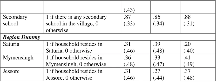
Figure 2 depicts how non-enrolment rates vary across boys and girls. This figure shows an opposite picture of the conventional belief that boys receive more education than girls. Boy’s non-enrolment rate is higher than girls at all age except at age 14. This is probably because, in recent times, the government of Bangladesh introduced an incentive program with the help of World Bank to increase girl’s school enrolment. From the age of 5 years, non-enrolment rates steadily decline to age 11 years for both boys and girls before it increases again. Girl’s non-enrolment rises to 17.7 per cent at age 14 years, whereas, boy’s enrolment is 14 per cent at the same age. At the age of 13, boys’ non-enrolment rate is much higher than that of girls; probably boys enter into the labour market from this age. Girl’s non-enrolment rate again rises sharply from the age of 15. At the age 17, girl’s non-enrolment rate is greater than boys. This possibly reflects the fact that girls have married or have withdrawn from school.
During the survey the children are asked ‘Are you still going to school?’ Only 67.8 per cent children of the total sample respond that they are attending school, while 2.2 per cent children report that they are attending school sometimes. On the other hand, 8.5 per cent children report that they are not going to school. However, for 21.4 per cent children, the information about their schooling is missing. In the sample, 74 per cent children are being educated in a co-education school and average distance of the nearest school from residence is between .25-.5 miles. Around 76 per cent children walk to school in all seasons. About 66per cent of the children study at the formal public school, while 2.7 per cent children study at formal madrasha8 and remaining children receive non-formal education.
4.2. Reason for Drop out from School
For the children not currently attending school the main reason for leaving school has been reported in the data. Table 4 reports the causes of leaving school for 5-17 years old children. Children that dropped out of school (about 8.8 per cent of the total sample) are asked the reason for dropping out from school; 27 per cent leave school because their parents couldn’t afford the expense; 27 per cent do not want to go to school; 13 per cent are deprived of schooling because their labour is essential for household work; and, another 4.2 per cent children leave school because of working in the own farm or for other income generating activities. Another reason for dropping out is that parents are reluctant to send girls to school, which account for 8.3 per cent of total drop out. Many parents in Bangladesh believe that it is not appropriate to send girls to school. Religious beliefs strengthen their view of not sending girls outside their home after a certain age.
4.3 Measurement of Children’s Work
The survey asks question about primary occupation and secondary occupation of all household members. To classify children’s activities, however, we focus on the occupation of children reported by household head. We define work broadly by including non-wage work and housework.
8
We consider two occupations (primary and secondary occupation) as the key indicators to define child work. Work and study are not mutually exclusive categories; as we see in the data, some children are reported attending school, while at the same time they are performing some form of paid or unpaid work. So we create four mutually exclusive categories to define child’s activity. These categories are - study only, work only, work and study, neither work nor study. We classify the children, in “study only category”, if their primary and secondary occupation is student or they do not have a secondary occupation. Similarly, “work only” category includes those children whose primary and secondary occupation is work or they do not have any secondary occupation but their primary occupation is definitely work. If a child works and attends school as well are included in “work and study” category. Neither work nor study category considers those who are reported as child in the survey. Presumably, they are neither going to school nor engaged in work, although there are in school going age.
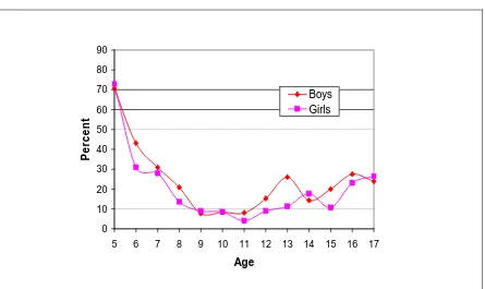
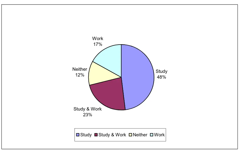
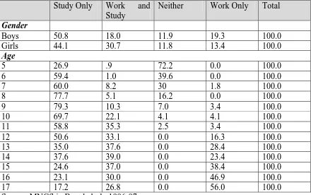
The figure 4 shows that only 48 per cent children attend school as their only activity. This represents 50.8 per cent of all boys and 44.1 per cent of all girls (Table 6). As seen from figure 4, another 17 per cent children are engaged in work as their only activity. Table 6 shows that this figure is 19.3 per cent for all boys and 13.4 per cent for all girls. Another 23 percent combine schooling with work.
4.4 Profile of Child Activity
Figure 4 indicates that 17 per cent children are reported to be engaged in paid or unpaid work. Household work is also included in the work category. Household is a common place for child work in rural Bangladesh. Most of the children are engaged in household work in rural areas, where agricultural work is performed mainly by the male children and household work is mainly performed by the female children. There are about 6 per cent children who are reported to be engaged in household work as their primary activity, where most of the children (about 4.6 per cent of the total children) are female children. In secondary occupation, about 15.4 per cent children, are reported to be performed household work as their secondary job, where 11.8 per cent are female children. Exclusion of household work therefore would seriously underestimate the work commitment of children, particularly for female children, which motivate us to include housework in the definition of child work.
Data from this survey reveals that children begin to work from 5 years of age. Children’s work participation increases with the age. Particularly, from 12 years old, work participation rate increases sharply, and school attendance falls increasingly. Increasing trend of children’s work participation with the age is because as children grow up their potential earning and opportunity cost of schooling increase with the age. School attendance is higher among 6-11 years old. On the other hand, neither schooling nor working children are prominent among the younger children aged from 5-11 years. Combining school with work also increases with the age up to 15 then decreases.
6. Empirical model and Estimation Issues
The multinomial logit model is used to estimate simultaneously the determinants of ‘work’, ‘study’, combining both, or doing neither.
Let Yi denote the polytomous variable with multiple unordered categories. Suppose there are j mutually exclusive categories and P Pi1 i2...Pij are the
probabilities associated with jcategories. In this case, we have four categories (j=4); 0
1
j= If child works and attends school, 2
j= If the child neither work nor study, 3
j= If the child works only.
Here, we consider study as reference category. These choices are associated with the following probabilities:
0
i
P = probability of study (not working)
1
i
P = probability of combining study and work
2
i
P = probability of neither work nor study
3
i
P = probability of work (not attending school).
0
1 2 3
1 1
1 2 3
2 2
1 2 3
3 3
1
( 0 ) ,
1 exp( ) exp( ) exp( )
exp( )
( 1 ) ,
1 exp( ) exp( ) exp( )
exp( )
( 2 ) ,
1 exp( ) exp( ) exp( )
exp( )
( 3 )
1 ex
r i i i
i i i
i
r i i i
i i i
i
r i i i
i i i
i
r i i i
P y x P
x x x
x
P y x P
x x x
x
P y x P
x x x
x
P y x P
β β β
β
β β β
β
β β β
β = = = ′ ′ ′ + + + ′ = = = ′ ′ ′ + + + ′ = = = ′ ′ ′ + + + ′ = = =
+ p(x′iβ1) exp(+ xi′β2) exp(+ xi′β3)
where β β1, 2and β3are the covariate effects of response categories study and work, neither work nor study and work only respectively with reference category study ( j=0) where β0= 0.
In general, for an outcome variable, Yiwith jcategories, the probability can be modelled as: 3 1 1 exp( ) ( )
1 exp( )
i
r i i ij j
i j j
x P y j x P
x β β − = ′ = = = ′ +
∑
for j;0
and (2)
0 1
1
1
( 0 )
1 exp( )
r i i i j
i j j
P y x P
Now, we estimate the above model for the sample size n. Each of n individuals falls into one of the j categories, with the probabilities given by (2). Let xibe the vector of explanatory variables, such as child, family and community characteristics. Thus for a model of k covariates, a total of (k+1)*(j-1) parameters are to be estimated. Then we usexito see the propensity of i towards j.
6.
Estimation and Empirical Findings
In empirical analysis, time use by children in different activities is used as dependent variable. Time use is represented by a variable taking value 0 if the child is reported attending school; 1 if the child attends school and works, 2 if child neither works nor attends school; and, 3 if the child works only. Explanatory variables used for the empirical investigation of the time use of school-age children mostly reflect the covariates in eq (8) of section 2.
To model the child’s activity choices a multinomial logit model is estimated for the probability that a child will “work only”, or combine both, or be in “neither” category as against “study only”. The estimated coefficient, t-statistics and odds ratios of multinomial logit are reported in the Table 6-8. Table 6 presents the results of all children, while Table 7 and Table 8 show the result for boys and girls separately. We estimate the sample separating by gender to see if there are any gender specific impacts on child labour decision.
6.1 Child’s characteristics
Child characteristics, such as age, gender, and whether the child is son/daughter of the head, appear to be important determinants of child labour and schooling decision. First let us consider the effect of age. The age coefficient is found to be significant for all categories (“work and study”, “neither” and “work”) as well as the boys’ sample. The probability of working and ‘combining work and study’ increases with age9. One
9
explanation of this result is that older children either have completed their studies or failed to continue. It may be also the case, as children grow up they acquire more experience and more human capital which creates a prospect of higher wages that induces them to leave school. However, insignificant age coefficient of ‘work only’ category in girls sample implies that age has no impact on the probability of working for girls (Table 8). The significant negative age coefficient of ‘neither work nor study’ indicates that younger children are more likely to be in neither category. This finding tells a different story in case of Bangladesh whereas studies from other developing countries finds that older children are more likely to be in neither category10. Levison et al.’s (2001) study in Mexico find no significant effect of age on the probability of combining work and study and on the probability on “neither work nor study”.
Table 6-8 confirm that if a child is the son or daughter of the head of household, he or she is more likely to specialise in study and less likely to specialize in work. This can be explained differently that if a child is not the son or daughter of the head, his or her odds to specialise in work are (1/exp (-2.221)=) 9.22 times as greater as that of a child of the head of household. This coefficient shows significant positive effect on the probability of combining work and study, which implies that son and daughter of the household head is also likely to combine study and work as opposed to the children of other relatives of the household head. This reflects that household head favours his/her own child with schooling or at least to combine school and work.
Now let us turn into gender coefficient. Although the gender coefficient has no effect on the probability of working and on the probability that a child will neither study nor work (Table 6); it has significant effect on the probability of combining study and work. Female children are more likely to combine study with work, since the odds of combining study with work for girls are nearly 3 times as higher as those of boys. This result is not surprising, as we include housework in the definition of work. It is thus show that probability of full time working decreases for the children up to 8 years old, then increases with the age up to age 12, then decreases again.
10
consistent with the finding of Levison, et al.’s (2001) who also find that if housework is included in the measurement of work, then, girls are 14.1 per cents points more likely than boys to combine work and study. However, other studies (for example, Grootaert, 1999; Maitra and Ray, 2002; Cigno and Rosati, 2000) that use conventional definition of work find that girls are less likely than boys to combine work and study.
6.2 Parents Characteristics
Among parental characteristics, both the education of father and mother and the occupation of father, have the greatest impact on child labour and schooling decision. Consistent with the theoretical assumption, empirical findings also reveal that the higher level of education of parents’ increases the likelihood that a school-age child will specialise in study relative to the likelihood that the child will “work only” or do neither. For example, the odds of working or doing nothing as opposed to schooling for children from illiterate father (used as reference category) are respectively (1/exp (-.902)) 2.47 and (1/exp (-1.205) 3.33 times as great as those from better-educated father (who can sign and write) (Table 6). On the other hand, relative to children from better educated mother (who can sign and write), children from illiterate mother are 1.55 times more likely to combine study with work, 4.49 times more likely to be in neither category, and 2.23 times more likely to work fulltime as opposed to study fulltime.
Among other parental variables, age of the parents is found to be insignificant. Some of the coefficients of occupation variable, however, give significant results. For example, if father’s occupation is trade, then it is more likely for the child to specialise in schooling. This gives the expected results that are predicted in the theoretical model. If a father is engaged in trade then positive income effect dominates to keep the children in the school. On the other hand, if the father of a child is day labourer or wage labourer, then it reduces the probability that the child will ‘study only’ and increases the probability that the child will combine ‘study and work’ or ‘work only’. For example, relative to reference category (father occupation is farming), children of day/wage labourer are nearly one and half times more likely to combine study with work, or doing nothing and nearly three time more likely to work fulltime (Table 6).
The mother occupation is found to be insignificant in the combined sample and boys sample. In case of girls, however, having a mother who does housework increases the likelihood that she specialises in schooling (Table 8). If mother does housework, then, it relieves girls from housework and makes it convenient for them to utilise their extra time to study. Parents’ occupations have no impact on the probability of “neither work nor study”.
6.3 Household Characteristics:
by girls. In that case schooling of girls becomes part time instead of fulltime. Theory also assumes that additional number of pre-school child tends to withdraw school-age children from schooling to work by the increased demand for child care time or by the increased cost of raising pre-school children. This study, however, confirms that reduced schooling is incurred by addition demand of childcare time rather than increasing cost of raising pre-school children. Hence, the finding suggests that pre-school children generate work for the school-age girls, as they require constant supervision and tending. The empirical result, however, contradicts with the theoretical prediction that the number of school-age children influences the probability of working and schooling, as the impact of the number of school-age children is found to be insignificant.
Cost of schooling variables are found to be insignificant, but where significant, it gives an unexpected sign. The regional dummies indicate that children residing in Mymensing and Jessore are more likely to work fulltime relative to children from Saturia.
7. Concluding Remarks
This paper analyses the incidence and determinants of child labour and school attendance in Bangladesh. The empirical findings provide evidence that the education of parents significantly increases the probability that a school-age child will specialise in study. Empirical results also show that if the father is employed in a vulnerable occupation, for example, day-labour or wage-labour, it raises the probability that a child will work full time or combine work and study. An increase in the number of total household members is associated with a higher probability of schooling.
Most of the literatures on child labour in developing countries find that boys are more likely to combine study and work. However, the significant and positive gender coefficient of this paper suggests that girls are more likely than boys to combine schooling with work in Bangladesh. Most of the girls in study areas are engaged in household work that allows them to combine school and work; because household work is more flexible than formal wage earning jobs. Another interesting finding of this study is that the analysis of the data shows that girl’s enrolment rate is higher than boys at all ages. This is probably because there is an on going education subsidy program for girls education in Bangladesh that attracts parents to send their daughter to school. This may be one reason why we have not found enough evidence of gender difference in child labour and school attendance.
paid to children of less educated and poor parents (estimated by occupation); as they can not afford schooling. We also find that the children who are not the sons and daughters of the head of household are more likely to work than the sons/ daughter of the household head. This may reflect the fact that if the household head is resource constrained then it is more likely for him to choose his own child for schooling first. This finding further sheds light on the relationship of child labour and poverty. Although this study could not provide any specific direction on the conjunction of child labour and household welfare, it tries, however, to indicate that child labour is negatively related with household income and welfare that is proxied by both the occupation and education of parents.
References
BBS. (1996).“Statistical Pocket Book of Bangladesh.” Bangladesh Bureau of Statistics (BBS), Dhaka.
BBS. (1997).“Statistical Year Book of Bangladesh.” Bangladesh Bureau of Statistics (BBS), Dhaka.
Becker, G. S. and Lewis, H. G. (1973). “On the Interaction between the Quantity and Quality of Children.” Journal of Political Economy, 81(2), Part 2, S279-S288. Becker, G. S. (1965). “A Theory of the Allocation of Time.” Economic Journal, 75,
493-517.
Blunch, N.-H. and Verner, D. (2000). “Revisiting the Link between Poverty and Child Labour: The Ghanaian Experience.” Mimeograph, The World Bank.
Browning M. and Chiappori P.A. (1998). “Efficient Intra-Household allocations: A General Characterization and Empirical Tests.” Econometrica, 66 (6), 1241-1278. Cartwright, K. (1999). “Child labour on Colombia.” Ch. 4 in Grootaert and Patrionos
(1999, eds)
Chiappori P.A. (1992). “Collective Labor Supply and Welfare.” The Journal of Political Economy, 100, 3, 437-467.
Cigno, A. and Rosati, F. C. (2000). “Why do Indian Children Work, and is it Bad for Them?” IZA Discussion Paper No. 115.
Dasgupta, P. (1995). An Inquiry Into Well-being and Destitution, Oxford, Clarendon Press.
Detray, D. N. (1973). “Child Quality and the Demand for Children.” Journal of Political Economy, 81, S70-S95.
Duraisamy, M. (2000).“Child Schooling and Child Work in India” Paper presented in the Eighth World Congress of the Econometric Society, August 11-16.
Emerson, P. M. and Portela, A. (2001). “ Bargaining Over Sons and Daughters: Child Labor, School Attendance and Intra-household Gender Bias in Brazil.” Working Paper, University of Colorado at Denver.
Grootaert, C. (1999). “Child Labour in Cote d Ivorie” Ch.3 in ‘ The Policy Analysis of Child Labour: A Comparative Study’ ed. Grootaert, C and Patrinos H.A. (1999), St. Martin Press, New York.
Ilahi, N. (2000). “The Intra-household Allocation of Time and Tasks: What Have We Learnt from the Empirical Literature?” Policy Report on Gender and Development, Working Paper Series No.13, The World Bank.
ILO. (1997a).“Combatting the Most Intolerable Forms of Child labour: A Global Challenge in the Report on Combating the Most Intolerable Forms of Child Labour: A global Challenge, Amsterdam, Child Labour Conference, Ministry of Social Affairs and Employment, The Hague.
ILO. (1997b). “Statistics on Working Children and Hazardous Child Labour in Brief, Bureau of Statistics, ILO, Geneva.
ILO-IPEC. (2002). “Every Child Counts: New Global Estimates on Child Labour.” International Labour Office, Geneva.
Khandker, S. R.(1988). “Determinants of Women’s Time Allocation in Rural Bangladesh.” Economic Development and Cultural Change, 37, 111-126.
Levison, D., Karine, S. M. and Felicia, M. K. (2001). “Youth Education and Work in Mexico.” World Development 29(1): 167-188.
Maddala, G.S. (1983). “Limited Dependent and Qualitative Variables in Econometrics.” Cambridge University Press, Cambridge.
Maitra, P. and Ray, R. 2002. “The Joint Estimation of Child Participation in Schooling and Employment: Comparative Evidence from Three Continents”. Oxford Development studies 30(1): 41-62.
Ridao-Cano, C. (2001) “Child Labor and Schooling in a Low Income Rural Economy.” University of Colorado, mimeo.
Rosenzweig, M. and Evenson, R (1977). “Fertility, Schooling and the Economic Contribution of Children in Rural India: An Econometric Analysis.” Econometrica, 45.
Salahuddin, K. (1981). "Aspects of Child Labour in Bangladesh." In ‘Disadvantage Children in Bangladesh: Some Reflections’ Women for Women, Dhaka, Bangladesh.
Sinha, N. (2003). “Fertility, Child Work and Schooling Consequences of Family Planning Programs: Evidence from an Experiment in Rural Bangladesh.” Center Discussion Paper No.867, Economic Growth Center, Yale University.
Table 1: Characteristics of the Micro Nutrient and Gender Study (First Round), 1996-97.
Characteristics Saturia Mymensingh Jessore All
Households 313 320 324 957
Individuals 1680 1923 1661 5264
Children (0-17) 726 827 703 2256
Children of the Household Head 581 657 589 1827
Children (5-17) 554 625 561 1740
Children of the Household Head 459 503 476 1438 Source: MNGS in Bangladesh, 1996-97.
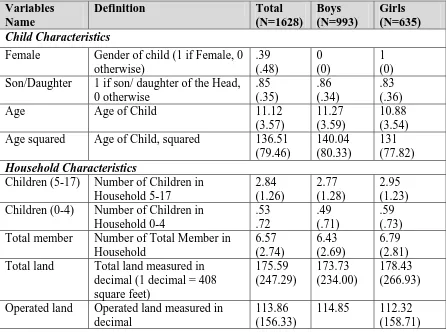
Table2: Variable names and definitions, means and standard deviations (standard deviation in parentheses under means) of variables.
Variables Name
Definition Total
(N=1628) Boys (N=993) Girls (N=635) Child Characteristics
Female Gender of child (1 if Female, 0 otherwise) .39 (.48) 0 (0) 1 (0) Son/Daughter 1 if son/ daughter of the Head,
0 otherwise .85 (.35) .86 (.34) .83 (.36)
Age Age of Child 11.12
(3.57)
11.27 (3.59)
10.88 (3.54) Age squared Age of Child, squared 136.51
(79.46) 140.04 (80.33) 131 (77.82) Household Characteristics
Children (5-17) Number of Children in Household 5-17 2.84 (1.26) 2.77 (1.28) 2.95 (1.23) Children (0-4) Number of Children in
Household 0-4 .53 .72 .49 (.71) .59 (.73) Total member Number of Total Member in
Household 6.57 (2.74) 6.43 (2.69) 6.79 (2.81) Total land Total land measured in
decimal (1 decimal = 408 square feet) 175.59 (247.29) 173.73 (234.00) 178.43 (266.93) Operated land Operated land measured in
decimal
113.86 (156.33)
(154.86) Homestead Homestead measured in
decimal 21.26 (24.14) 21.41 (23.69) 21.04 (24.85) Parental Characteristics
Father age Age of father 46.86
(10.57)
47.01 (10.75)
46.61 (10.28) Father’s Education Dummy
Illiterate 1 if father is illiterate, 0 otherwise .26 (.44) .26 (.44) .25 (.43) Can sign only 1 if father can sign only, 0
otherwise .27 (.44) .27 (.44) .26 (.44) Can read only 1 if father can read only, 0
otherwise .02 (.16) .02 (.16) .02 (.16) Can read and
write
1 if father can read and write, 0 otherwise .43 (.49) .43 (.49) .45 (.49) Father’s Occupation Dummy
Farming 1 if father’s occupation is agriculture, 0 otherwise
.48 (.49) .48 (.49) .47 (.49) Service 1 if father’s occupation is
service, 0 otherwise
.11 (.32) .11 (.32) .12 (.33) Trade 1 if father’s occupation is
business, 0 otherwise
.16 (.37) .16 (.37) .16 (.37) Day/wage labourer
1 if father is day labour and wage labour, 0 otherwise
.19 (.39) .19 (.39) .21 (.40) Other Occupation
1 if father is engaged in other occupation than the occupation stated above, 0 otherwise
.03 (.18) .03 (.18) .02 (.15)
Mother Age Age of mother 38.01
(9.21)
38.12 (9.27)
37.84 (9.12) Mother’s Education Dummy
Illiterate
1 if mother is illiterate, 0 otherwise .36 (.48) .39 (.48) .31 (.46) Can sign only 1 if mother can sign only, 0otherwise .36 (.48) .34 (.48) .39 (.48) Can read only 1 if mother can read only, 0
otherwise .04 (.20) .03 (.17) .05 (.23) Can read and
write
1 if mother can read and write, 0 otherwise .23 (.42) .23 (.42) .23 (.42) Mother’s Occupation
1 if mother does housework, 0 otherwise .94 (.22) .94 (.23) .95 (.21) Cost of Education
Distance to primary school
Distance to the nearest primary school
.25 .28 (.46)
(.43) Secondary
school
1 if there is any secondary school in the village, 0 otherwise
.87 (.33)
.86 (.34)
.88 (.31) Region Dummy
Saturia 1 if household resides in Saturia, 0 otherwise
.31 (.46)
.39 (.48)
.20 (.40) Mymensingh 1 if household resides in
Mymensingh, 0 otherwise
.36 (.48)
.33 (.47)
.41 (.49) Jessore 1 if household resides in
Jessore, 0 otherwise
.31 (.46)
.27 (.44)
[image:29.612.84.534.71.241.2].37 (.48)
Table 3: Enrolment in Primary School (1995-2001)
Source: Primary and Mass Education Division. Year Total (in
million)
Boys (percent)
Girls (percent)
1995 17.2 52.6 47.8
1996 17.5 52.8 47.6
1997 18.0 51.9 48.1
1998 18.3 52.1 47.8
1999 17.6 51.8 48.6
2000 17.6 51.3 48.7
Figure 1: Children not enrolled in School by Age
0 10 20 30 40 50 60 70 80 90
5 6 7 8 9 10 11 12 13 14 15 16 17
Age
P
e
rcen
t
Source: MNGS in Bangladesh, 1996-97.
Figure 2: Children not Enrolled in School by Age and Gender
0 10 20 30 40 50 60 70 80 90
5 6 7 8 9 10 11 12 13 14 15 16 17
Age
Per
c
ent
Boys Girls
[image:30.612.85.530.433.698.2]Table 4: Reason for Leaving School.
Cause Percent
Couldn’t Afford 27.1
Sickness 4.2
Needed for Housework 13.2
Needed for Own Farm .7
Needed for Income Generating Activities 3.5
School too Faraway 6.9
Not Appropriate to send girls to School 8.3
Did not Want to Go 27.1
Other Reason 9.0
Total 100 Source: MNGS in Bangladesh, 1996-97.
Figure 3: Distribution of Children across Four Categories (%).
Study 48%
Study & Work 23% Neither
12% Work
17%
Study Study & Work Neither Work
[image:31.612.91.486.411.658.2]Table 5: Activity Status of Children across Gender and Age (in per cent). Study Only Work and
Study
Neither Work Only Total Gender
Boys 50.8 18.0 11.9 19.3 100.0 Girls 44.1 30.7 11.8 13.4 100.0 Age
5 26.9 .9 72.2 0.0 100.0
6 59.4 1.0 39.6 0.0 100.0
7 60.0 8.2 30 1.8 100.0
8 77.7 5.1 16.2 0.0 100.0
9 79.3 10.3 7.0 3.4 100.0
Table 6: Multinomial logit estimates for all children (The reference category is Study only).
Study and Work Neither Work
Variable Names Coefficient t-statistics
Odds-ratio
Coefficient t-statistics
Odds-ratio
Coefficient t-statistics
Odds-ratio
Constant -9.252 -6.084 9.106 4.750 -12.495 -4.378
Child Characteristics
Female 1.037 6.659 2.82 -.017 -.078 0.983 -.174 -.815 .840
Son/Daughter .595 1.970 1.81 -.158 -.358 0.853 -2.221 -8.075 .108
Age 1.156 5.069 3.177 -1.43 -3.603 0.239 1.451 3.500 4.267
Age squared -.031 -3.379 .969 .034 1.407 1.034 -.029 -1.884 .971
Household Characteristics
Children (5-17) .039 .475 1.039 .223 1.759 1.249 -.010 -.114 .990
Children (0-4) .340 2.760 1.404 -.061 -.326 0.940 .102 .619 1.107 Total member -.130 -2.641 .87 .028 .397 1.028 -.112 -1.937 .894 Total land .000 1.038 1 -.001 -1.656 0.999 -.000 -.084 1
Operated land .002 1.950 1.002 -.002 -1.292 .998 -.000 -.026 1
Homestead -.006 -1.622 .994 .019 2.389 1.019 -.005 -1.208 .990
Parents Characteristics
Father age -.017 -1.017 .983 -.022 -.822 0.978 .029 1.577 1.029
Father’s Education (ref.: Illiterate)
Can sign only .006 .028 1.006 -.790 -2.755 0.453 -.607 -2.296 .544 Can read only .540 1.112 1.716 -1.064 -1.279 0.345 .242 .387 1.273 Can read and write -.358 -1.629 .699 -1.205 -3.845 0.299 -.902 -3.369 .405
Father Occupation (ref.: Farming)
Service -.364 -1.437 .694 .110 .248 1.116 -.438 -1.291 .645
Trade -.565 -2.449 .568 .229 .726 1.257 .006 .023 1.006
Mother Age .015 .736 1.015 .003 .084 1.003 -.020 -.916 .980
Mother Education (ref.: Illiterate)
Can sign only -.227 -1.251 .796 -.399 -1.566 .670 -.609 -2.632 .543 Can read only -.299 -.738 .741 -.798 -1.250 .450 -.611 -1.094 .542 Can read and write -.439 -1.922 .644 -1.500 -3.966 .223 -.802 -2.726 .448 Mother’s
Occupation
-.332 -1.019 .717 -.087 -.164 .916 .063 .156 1.065
Cost of Education
Distance to primary school
-.188 -1.040 .828 .279 1.057 1.321 -.0705 -.322 .932
Secondary school .003 .013 1.003 -.033 -.093 .967 .410 1.278 1.506
Region Dummies (ref.: Saturia)
Mymensingh -.016 -.079 .984 .166 .564 1.180 .497 1.903 1.644
Jessore -.061 -.321 .940 -1.117 -3.793 .327 .523 2.155 1.687
Chi squared 1471.672 (d.f.81) Pseudo R-squared .363
Table 7: Multinomial Logit Estimates for Boys (The reference category is Study only).
Study and Work Neither Work
Variable Names Coefficient t-statistics
Odds-ratio
Coefficient t-statisti
cs
Odds-ratio
Coefficient t-statistics
Odds-ratio
Constant -7.727 -3.568 8.227 3.461 -12.496 -3.665
Child Characteristics
Son/Daughter .673 1.459 1.960 .119 .202 1.126 -2.128 -6.162 0.119 Age .931 2.904 2.537 -1.39 -2.794 .249 1.401 2.840 4.059 Age squared -.022 -1.749 .978 .032 1.071 1.032 -.028 -1.514 .972
Household Characteristics
Children (5-17) .130 1.133 1.138 .101 .640 1.106 .011 .093 1.011 Children (0-4) .014 .081 1.014 -.061 -.250 .940 -.028 -.140 .972
Total member -.068 -.969 .934 .020 .215 1.020 -.088 -1.197 .915 Total land -.000 -.355 1 -.003 -2.132 .997 -.000 -.800 1
Operated land .002 1.974 1.002 -.000 -.431 1 .000 .279 1
Homestead -.002 -.283 .998 .028 2.995 1.028 -.003 -.482 .997
Parents Characteristics
Father age -.031 -1.330 .969 -.014 -.401 .986 .034 1.520 1.034
Father’s Education (ref.: Illiterate)
Can sign only -.176 -.630 .838 -.877 -2.370 .416 -.655 -2.077 .519 Can read only .500 .809 1.648 -.850 -.846 .427 .284 .369 1.328 Can read and write -.554 -1.874 .574 -1.028 -2.591 .357 -.917 -2.776 .399
Father Occupation (ref.: Farming)
Service -.470 -1.277 .625 .585 1.015 1.794 -.659 -1.618 .517
Trade -.912 -2.732 .401 .398 .970 1.488 -.164 -.497 .848
Mother Age .019 .648 1.019 .001 .029 1.001 -.021 -.793 .979
Mother Education (ref.: Illiterate)
Can sign only -.373 -1.541 .688 -.580 -1.753 .559 -.579 -2.087 .560 Can read only .056 .094 1.057 -.810 -.830 .444 -.107 -.141 .898 Can read and write -.710 -2.209 .491 -1.692 -3.539 .184 -.624 -1.799 .535 Mother’s
Occupation
.000 .001 1 .109 .173 1.115 .691 1.406 1.995
Cost of Education
Distance to primary school
-.296 -1.288 .743 .266 .845 1.304 -.292 -1.122 .746
Secondary school -.002 -.008 .998 .127 .280 1.135 .137 .382 1.146
Region Dummy (ref.: Saturia)
Mymensingh -.641 -2.360 .527 .269 .704 1.309 -.043 .957 .697
Jessore -.466 -1.825 .628 -.668 1.808 .513 .359 .668 .668
Chi squared 863.2037 (d.f.78) Pseudo R-squared .355
Table 8: Multinomial Logit Estimates for Girls (The reference category is Study only).
Study and Work Neither Work
Variable Names Coefficient t-statistics
Odds-ratio
Coefficien t
t-statistics
Odds-ratio
Coefficient t-statistics
Odds-ratio Constant -10.525 -4.444 11.258 2.974 -12.73 -2.319
Child Characteristics
Son/Daughter .567 1.264 1.762 -.400 -.534 .670 -2.453 -4.749 .086
Age 1.306 3.659 3.691 -1.554 -1.948 .211 1.216 1.525 3.373
Age squared -.035 -2.324 .965 .036 .694 1.036 -.015 -.482 .985
Household Characteristics
Children (5-17) -.031 -.237 .969 .397 1.657 1.487 -.010 -.055 .990 Children (0-4) .850 4.153 .427 -.060 -.181 .941 .345 1.029 1.411 Total member -.212 -2.691 1 .090 .618 1.094 -.174 -1.608 .840
Total land .001 1.974 1 .000 .054 1 .001 .972 1
Operated land .000 .743 .987 -.004 -1.281 .996 .000 .235 1
Homestead -.013 -2.218 1.007 .005 .348 1.005 -.016 -1.800 .984
Parents Characteristics
Father age .007 .250 1.300 -.024 -.514 .976 .012 .289 1.012
Father’s Education (ref.: Illiterate)
Can sign only .263 .735 1.300 -.760 -1.539 .467 -.579 -1.068 .560 Can read only .228 .283 1.256 -.701 -.419 .496 .305 .270 1.356 Can read and write -.051 -.143 .950 -1.60 -2.909 .201 -.918 -1.805 .399
Father Occupation (ref.: Farming)
Service -.360 -.906 .697 -.584 -.692 .557 .460 .690 1.584
Trade -.370 -.985 .690 .181 .342 1.198 .432 .744 1.540
Mother Age .014 .433 1.014 -.013 -.220 .987 .002 .033 1.002
Mother Education (ref.: Illiterate)
Can sign only -.165 -.533 .847 -.172 -.388 .841 -.781 -1.685 .458 Can read only -.995 -1.672 .369 -1.060 -1.067 .346 -1.355 -1.485 .257 Can read and write -.147 -.396 .863 -1.496 -2.184 .224 -1.163 -1.880 .312 Mother’s
Occupation
-1.341 -2.185 .261 -.876 -.846 .412 -1.568 -1.781 .208
Cost of Education
Distance to primary school
-.008 -.026 0.992 -.038 -.071 .962 .647 1.419 1.909
Secondary school .298 .791 1.347 -.108 -.173 .897 1.944 2.085 6.986
Region Dummy (ref.: Saturia)
Mymensingh 1.237 3.386 3.445 -.110 -.213 .896 1.942 3.302 6.972
Jessore .931 2.648 2.537 -1.902 -3.573 .149 .955 1.657 2.599
Chi squared 671.4555 (d.f. 78) Pseudo R-squared .425