MULTI-OBJECTIVE CALIBRATION
FOR AGENT-BASED MODELS
Alex Rogers
Intelligence, Agents, Multimedia Group Electronics and Computer Science
Southampton, SO17 1BJ, UK
Peter von Tessin Eurobios UK 26 Farringdon Street London EC4A 4AB, UK
KEYWORDS
Agent based model, calibration, pareto-optimality, genetic algorithm.
ABSTRACT
Agent-based modelling is already proving to be an immensely useful tool for scientific and industrial modelling applications. Whilst the building of such models will always be something between an art and a science, once a detailed model has been built, the process of parameter calibration should be performed as precisely as possible. This task is often made dif-ficult by the proliferation of model parameters with non-linear interactions. In addition to this, these models generate a large number of outputs, and their ‘accuracy’ can be measured by many different, often conflicting, criteria. In this paper we demonstrate the use of multi-objective optimisation tools to cal-ibrate just such an agent-based model. We use an agent-based model of a financial market as an exem-plar and calibrate the model using a multi-objective genetic algorithm. The technique is automated and requires no explicit weighting of criteria prior to cal-ibration. The final choice of parameter set can be made after calibration with the additional input of the domain expert.
INTRODUCTION
Agent-based modelling and simulation is one of the most useful tools for understanding complex dy-namic systems. The properties of such systems, which are mostly the result of the agents actions and interactions, are much better understood when we build models of these systems from the bottom up. By such a procedure we gain insights into the work-ing of the entire system which would not have been possible by concentrating our analysis on only the in and out flow of data, as would be the case with traditional statistical models.
However, this approach often leads to a concentra-tion of the modelling efforts on the inner workings of the various agents and thus a proliferation of model parameters. These parameters often interact in an extremely complex, non-linear manner. Whilst the insights gained through this modelling work might be
very valuable, the usefulness of the resulting model is only assured if it can accurately reproduce phe-nomenon observed in the real system. Our model building often indicates how some of the model pa-rameters must be set, however we are typically left with a number of parameters which must be tuned
by comparing the predictions of the model against real world data.
The comparison of the model to real world data is often complicated by a number of factors. A suffi-ciently complex model produces a number of outputs and thus the ‘accuracy’ of the model can be measured by any number of different criteria. These criteria are often conflicting and thus, increasing the accuracy of one, results in the degrading of another. Addition-ally, there is often no cleara priori way of weighting one criteria against another. Also, the model often incorporate some form of stochastic events. Thus the model must not reproduce exact real world data, but it must be statistically similar to the real world data. Despite the importance of this calibration task, there are few systematic methodologies and the cal-ibration is typically done by hand (Manson, 2001; Palin, 2002). Where researchers have considered evo-lutionary algorithms to automatically update model parameters, there is typically only a single ‘accuracy’ criteria or a direct weighting over several criteria (Said et al., 2002).
In this paper, using a simple agent-based model of a financial market, we introduce the use of tech-niques from multi-objective optimisation to tune the parameters of the model. This technique is auto-mated and does not require that we explicitly trade-off one criteria against another. We use a genetic algorithm to run the model repeatedly with differ-ent parameter setting and we evolve a population of pareto-optimal parameters sets. From this popula-tion, we can then select a single candidate as our final tuned parameter set. The generation of a pop-ulation of pareto-optimal parameter sets, allows this final selection to be made in the presence of the do-main expert without any prior explicit weighting of criteria.
The remainder of the paper is organised as follows: in the following section we give a short description of the exemplar agent-based model and the various
agents it incorporates. We then describe the use of the multi-objective genetic algorithm for calibrating this model against real world stock price data. We present the results of this calibration and in the con-clusion discuss this the use of this technique in more general problems.
FINANCIAL MARKET MODEL
Our exemplar model is an agent-based model of a financial market (Farmer and Joshi, 2000). Unlike more complex models where agents bid on individ-ual assets (Arthur et al., 1997; Darley and Brown, 1999), it incorporates a market maker who drives the price discovery process depending on the net or-ders placed by a population of trading agents. These trading agents are split in two different categories – trend followers who act solely on their current ob-servation of the asset price and value investors who also consider a fundamental value for the asset. The intention of the Farmer and Joshi model is to show how simple trading strategies inside an agent-based model of a financial market can provide realistic look-ing asset price time-series. These time-series share some of the characteristics of real world asset prices (e.g. clustered volatility and unit roots). We go one step beyond the statement of such similarities and attempt to calibrate the parameters of the Farmer and Joshi model, in order to derive prices which are as statistically similar to real world prices as possi-ble. We give a sketch of agents here, although we recommend Farmer and Joshi’s original paper for a full account.
Market Maker
The market maker in the Farmer and Joshi model is risk neutral and determines the price of the traded asset by looking only at the supply and demand gen-erated by the population of N traders. A market impact function is used to describe the change in pt(the logarithm of the asset pricePt) at each time
step (Das, 2003). This market impact function is given by
pt+1=pt+
1 λ
N X
i=0
ωti+ξt+1 (1)
whereωi is the net demand per agent (i.e. the
num-ber of shares of the asset that the agent wishes to buy or sell). The market maker has a liquidity pa-rameter,λ, and in each period a small random term, ξt+1, drawn from a Gaussian, is used to capture all
the other possible influences on the price of the asset.
Trend Follower
The trend following investor assumes that the asset price has inertia and thus always continues to move in its current direction (i.e. it will continue to rise if it rose in the past and it will continue to fall if it
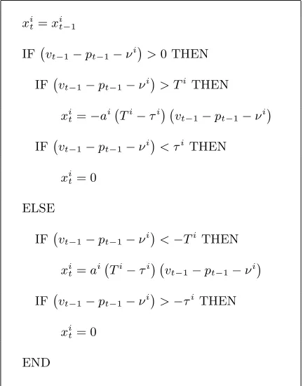
xit=xit−1
IF vt
−1−pt−1−ν
i
>0 THEN IF vt
−1−pt−1−ν
i
> TiTHEN
xit=−ai Ti−τi
vt−1−pt−1−ν
i
IF vt
−1−pt−1−ν
i
< τi THEN
xit= 0
ELSE IF vt
−1−pt−1−ν
i
<−TiTHEN
xit=ai Ti−τi
vt−1−pt−1−ν
i
IF vt
−1−pt−1−ν
i
>−τiTHEN
xit= 0
[image:2.595.333.549.72.347.2]END
Figure 1: Algorithm for calculating the position of the value investor.
fell in the past). Therefore her position (the number of shares of the asset held) in each period is propor-tional to the change in asset price determined over a fixed period of time
xit=a i
(pt−1−pt
−θi) (2)
whereθi
represents the time-lag over which the price movement is determined and ai
represents a scale parameter for capital assignment. The demand,ωi
t,
of the agent at this time is simply the change in her position and is thus given by
ωi t=x
i t−xit
−1. (3)
Value Investor
The value investor is a more sophisticated agent than the trend follower. She makes a subjective assess-ment of the value of the asset in relation to the cur-rent price of the asset. Her position is proportional to the difference between this fundamental value and the actual current market price
xit∝ vt−1−pt−1−νi (4)
where vt
−1 represents the logarithm of the asset
value, Vt
−1, and ν
i
Number of value agents Nvalue 100
Number of trend agents Ntrend 100
Min threshold for entering position Tvalue min 0.4
Max threshold for entering position Tvalue max 1.4
Min threshold for exiting position τvalue min -1.4
Max threshold for exiting position τvalue max -0.4
Scaling for capital assignment avalue 0.001
Scaling for capital assignment atrend 0.001
Min offset for perceived value νmin -0.10
Max offset for perceived value νmax 1.00
Min delay for trend followers θmin 20
Max delay for trend followers θmax 80
Price formation process noise σξ 0.01
Liquidity λ 0.50
[image:3.595.326.548.68.261.2]Starting price p0 0.20
Figure 2: Default model paramters.
Under this strategy, the value investors disregard their actual position. However, this disregard may lead to an unbounded value for this position; a situ-ation which would be contrary to any real world in-vestors behavior. For this reason Farmer and Joshi introduced thresholds into the value strategy, so that a value investor will only enter or exit a position when the difference between the perceived funda-mental value and the current price is beyond that threshold; otherwise the position remains unchanged from the last time period. To quote Farmer and Joshi, “Assume that a short position is entered when the mispricing exceeds a threshold Ti
and exited when it goes below a thresholdτi
. Similarly, a long position is entered when the mispricing drops below a threshold−Ti and exited when it exceeds−τi”.”
Figure 1 shows the algorithm for the decision mak-ing when these thresholds are incorporated. Again, the demand, ωi
t, of the agent at this time is simply
the change in her position and is thus given by
ωti=x i t−x
i t
−1. (5)
Running the Model
In order to run the model, the agents must be ini-tialised with their relevant parameters. In the case of a value investor, for example, these are ai
, νi
, Ti
andτi
. Rather than specify parameter values for ev-ery individual agent, Farmer and Joshi assign these values by drawing them from a uniform distribution where the model parameters specify the upper and lower bound of this uniform distribution. Figure 2 shows the default parameters which we are ulti-mately seeking to calibrate.
We do not have complete freedom over the choice of parameter values. As the correlation of log-returns (the change in asset price,pt−pt
−1) is close to zero
in real asset price time-series, the model should im-pose this feature. This is done by ensuring that the number of trend following agents matches the
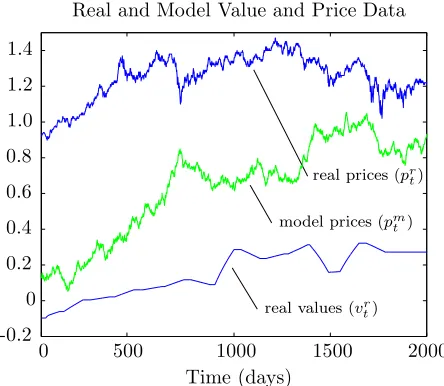
num-Real and Model Value and Price Data
Time (days)
model prices (pm t )
real prices (pr t)
real values (vr t)
0
0 500 1000 1500 2000
[image:3.595.81.291.73.234.2]-0.2 0.2 0.4 0.6 0.8 1.0 1.2 1.4
Figure 3: Real price and value data plotted with the model price output when run with default parame-ters.
ber of value investors and they share the same scaling constant for capital assignment.
In addition to initialising the agent parameters, we must provide a real asset value time-series, which acts as the driver for the value investors. As a proxy for this data, we use the earnings per share (EPS) of the asset, smoothed over a number of days to gener-ate a continuous curve. In the example runs of the model presented here, we use historical data covering eight years of daily data taken from an asset in the Euro-Stoxx-50TMindex 1.
Figure 3 shows the results of running the model with this input data and the default parameters. The ‘real value’ curve is the smoothed real world earning per share data. The ‘real price’ data is the real world share price data and the ‘model price’ curve is the model output.
MULTI-OBJECTIVE CALIBRATION
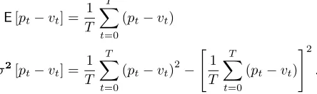
In order to calibrate the model, we must tune the parameters to ensure that the output matches the real asset price data. As the model itself is stochastic, we can not simply match the time-series, but must match the statistical properties of the time-series. Our choice of measure is driven by a feature of the model, that is, the price and value time-series are cointegrated (Jasiak and Gourieroux, 2002). Thus, whilst the price and value data may follow their own random walks, the value [pt−vt] is drawn from a
well defined distribution. Thus we attempt to match two criteria, the mean and variance of this [pt−vt]
1
distribution. These two criteria are thus given by
E[pt−vt] =
1 T
T X
t=0
(pt−vt)
σ2[pt−vt] =
1 T
T X
t=0
(pt−vt) 2
−
" 1 T
T X
t=0
(pt−vt) #2
.
We compareE[pm t −v
r
t] andσ2[p m t −v
r
t] calculated
using the model price time-series and the real value time-series with E[pr
t−v r
t] and σ2[p r t−v
r
t]
calcu-lated using the both the real price and real value time-series. As the model is driven by stochastic factors, we run the model a number of times (in this case, 100 times) in order to collect repeatable statis-tics.
We calculate the percentage error in the model price value compared to the real price values and these two criteria are used to judge the accuracy of the model output in our example. As it is not clear,a priori, how we should weight these two measures, we use multi-objective optimisation to find parameters sets which results in pareto-optimal combinations of two criteria.
There are a number of multi-objective optimisa-tion techniques, but the one we present here uses a multi-objective genetic algorithm to search for a population parameter sets which yield pareto-optimal combinations to the accuracy criteria (Flem-ing, 1993; Horn et al., 1994). The chromosomes of the genetic algorithm encode the parameters of the model. The chromosomes are evaluated by running the model with the encoded parameters and calcu-lating the accuracy criteria as described above.
The first two operators of the multi-objective ge-netic algorithm (i.e. mutation and crossover) are unchanged from the conventional genetic algorithm. We apply mutation to each individual by selecting one of the real coded model parameters and apply-ing a small random percentage change. Uniform crossover is performed by dividing the population into pairs and exchanging parameters between each pair with probability 1/2.
The significant difference between the multi-objective genetic algorithm and the conventional ge-netic algorithm occurs when selection is considered. In the conventional genetic algorithm, selection to the next generation requires a single ‘explicit’ fitness to be evaluated (Davis, 1991). The multi-object ge-netic algorithm differs from this standard algorithm in two important ways. Firstly, there is no need for this single ‘fitness’ value. Rather the solutions are sorted in order of pareto-dominance, where one solu-tion is dominated by another, if all the accuracy cri-teria of that solution are better. The next generation is selected on the basis of this ranking. Thus the pop-ulation member which is not dominated by any other, is most likely to be selected for the next generation.
Whilst the population member which is dominated by all the other solutions, will almost certainly not be selected. Like the conventional genetic algorithm, this selection scheme is stochastic. This changes alle-viates the need to explicitly weight different criteria in order to calculate a single ‘fitness’ value and also preserves diversity in the population, as two solu-tions with the same pareto-dominance ranking may actually encode very different parameter settings.
The second difference, is that all the solutions gen-erated are stored in an archive at the end of each generation and solutions which are dominated by any others are pruned from this archive. Thus the archive represents a store of parameter sets which yield pareto-optimal solutions to the calibration problem and the current population of the genetic algorithm is the source of new solutions.
RESULTS
The multi-objective genetic algorithm was initialised with a population of 20 parameter sets and run for 100 generations. Each evaluation of a parameter set involves running the model 100 times in order to ensure that the values ofE[pt−vt] and σ2[pt−vt]
[image:4.595.75.297.99.165.2]calculated, are repeatable. In general, there are no stopping criteria for the multi-objective genetic algo-rithm; whilst the population still shows some diver-sity, it is still effectively searching for new solutions. The limiting factor is the computational time avail-able.
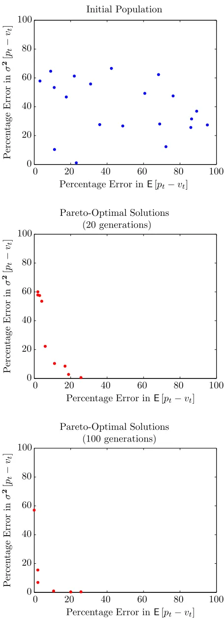
Figure 4 shows the initial population of parameter sets and the archive of pareto-optimal parameter sets after 20 generation and after 100 generations. The two plots of the archive, show how the pareto-optimal parameters sets form a line in the two dimensional space which gradually moves toward the bottom left corner, indicating that better and better solutions to the calibration problem are being found. The plots show some evidence of there being a trade-off in the accuracy criteria. It is possible to generate param-eters sets which very accurately match the value of
E[pt−vt] but at some sacrifice to the accuracy of
matching the value ofσ2[pt−vt].
The final contents of the archive is a population of parameter sets that yield non-dominated pareto-optimal solutions to the calibration problem. With no way to weight one criteria against the other, there is no explicit way to choose between them. However in sophisticated models, there are often other char-acteristics which have not been included as measur-able criteria but allow the domain expert to choose between them. In our example, this is not the case and we simply select a parameter set in the middle of the range where both criteria are well satisfied. Figure 5 shows these parameter values.
pre-Percentage Error inE[pt−vt]
P
er
ce
n
ta
g
e
E
rr
o
r
in
σ
2[
pt
−
vt
]
Initial Population
0 0 20
20 40
40 60
60 80
80 100
100
Percentage Error inE[pt−vt]
P
er
ce
n
ta
g
e
E
rr
o
r
in
σ
2[
pt
−
vt
]
Pareto-Optimal Solutions (20 generations)
0 0 20
20 40
40 60
60 80
80 100
100
Percentage Error inE[pt−vt]
P
er
ce
n
ta
g
e
E
rr
o
r
in
σ
2[
pt
−
vt
]
Pareto-Optimal Solutions (100 generations)
0 0 20
20 40
40 60
60 80
80 100
100
Figure 4: Sequence showing the development of pareto-optimal parameter sets during subsequent generations of the multi-objective genetic algorithm.
Number of value agents Nvalue 120
Number of trend agents Ntrend 120
Min threshold for entering position Tvalue
min 0.18
Max threshold for entering position Tvalue
max 2.73
Min threshold for exiting position τvalue
min -0.32
Max threshold for exiting position τvalue
max -0.13
Scaling for capital assignment avalue 0.0001
Scaling for capital assignment atrend 0.0001
Min offset for perceived value νmin -1.95
Max offset for perceived value νmax 0.75
Min delay for trend followers θmin 1
Max delay for trend followers θmax 120
Price formation process noise σξ 0.01
Liquidity λ 0.41
[image:5.595.332.549.72.234.2]Starting price p0 1.08
Figure 5: Final calibrated model paramters.
Real and Model Value and Price Data
Time (days)
model prices (pm t )
real prices (pr t)
real values (vr t)
0
0 500 1000 1500 2000
[image:5.595.65.293.74.702.2]-0.2 0.2 0.4 0.6 0.8 1.0 1.2 1.4
Figure 6: Real and model price data plotted against time. Value data also plotted.
vious run presented, where the default parameters were used. Whilst we have not attempted to match the actual time-series, the statistical properties of both the model and real price time series show good agreement.
CONCLUSIONS
[image:5.595.329.550.277.470.2]the need to explicitly trade-off one criteria against another and this final decision can often be made with the assistance of the domain expert.
We demonstrated the process with a simple agent-based model of a financial market. This model shares many of the properties of larger more complex agent-based models used in real applications. It involves a large number of parameters that interact in a non-linear manner. As the model incorporates stochastic effects, we can not simply compare the model out-puts to the real world equivalent, but must match the statistical properties of both. This typically in-volves running the model repeatedly to ensure that these statistical measures are repeatable. It is the computational time required to perform these runs which tends to be the limiting factor in the process. In the example agent-based model presented, we derived two criteria for comparing the accuracy of the model output to the real world asset prices. The resulting population of pareto-optimal thus repre-sents a line in the two dimension plot. Where there are more criteria, the population represents a surface in some high dimensional space. Visualising this re-sult becomes more complex and we are currently in-vestigating visualisation tools to aid in this process.
REFERENCES
Arthur, B., Holland, J., LeBaron, B., Palmer, R., and Tayler, P. (1997). Asset pricing under en-dogenous expectations in an artificial stock mar-ket. Addison-Wesley.
Darley, V. and Brown, M. (1999). The future of trad-ing: Biology-based market modeling at Nasdaq. InPerspectives in Business Innovation. Issue 4. Ernst and Young Center for Business Innova-tion.
Das, S. (2003). Intelligent Market-Making in Ar-tificial Financial Markets. PhD thesis, Mas-sachusetts Institure of Technology.
Davis, L., editor (1991). Handbook of Genetic Algo-rithms. Van Nstrand Reinhold, New York.
Farmer, J. and Joshi, S. (2000). The price dynamics of common trading strategies. Technical report, SFI Working Paper 00-12-069, Santa Fe Insti-tute.
Fleming, C. M. F. . P. J. (1993). Genetic Algorithms for Multiobjective Optimisation: Formulation, Discussion and Generalisation. In Proceedings of 5th International Conference on Genetic Al-gorithms, pages 416–423. Morgan Kaufmann.
Horn, J., Nafpliotis, N., and Goldberg, D. E. (1994). A niched Pareto Genetic Algorithm for Multi-objective Optimisation. InProceedings of IEEE Conference on Evolutionary Computation, vol-ume 1, pages 82–87. IEEE.
Jasiak, J. and Gourieroux, C. (2002). Financial Econometrics. Princeton University Press.
Manson, S. (2001). Calibration, Verification, and Validation. InMeeting the Challenge of Com-plexity. Proceedings of a Special Workshop on Land-Use/Land-Cover Change. Center for the Study of Institutions, Population, and Environ-mental Change.
Palin, J. (2002). Agent-Based Stockmarket Models: Calibration Issues and Application. PhD thesis, University of Sussex, UK.
Said, L. B., Bouron, T., and Drogoul, A. (2002). Agent-based interaction analysis of consumer behavior. In Proceedings of the first interna-tional joint conference on Autonomous agents and multiagent systems, pages 184–190. ACM Press.
AUTHOR BIOGRAPHIES
ALEX ROGERS is a Senior Research Fellow in the Intelligence, Agents, Multimedia Group at the University of Southampton. He gained a Ph.D. for work modelling the dynamics of genetic algorithms and has worked with Eurobios UK on a number of business consulting and agent-based nodelling projects. His email address is