Spectroscopy of K
¿"
Rg and transport coefficients of K
¿in Rg
„
Rg
Ä
He–Rn
…
Larry A. Viehlanda)
Division of Science, Chatham College, Pittsburgh, Pennsylvania 15232
Je´roˆme Lozeilleb)
Department of Chemistry, University of Sussex, Falmer, Brighton, United Kingdom BN1 9QJ
Pavel Solda´n
Department of Chemistry, University of Durham, South Road, Durham, United Kingdom DH1 3LE
Edmond P. F. Leec)
School of Chemistry, University of Southampton, Highfield, Southampton, United Kingdom SO17 1BJ and Department of Applied Biology and Chemical Technology, Hong Kong Polytechnic University, Hung Hom, Hong Kong
Timothy G. Wrightd)
Department of Chemistry, University of Sussex, Falmer, Brighton, United Kingdom BN1 9QJ 共Received 6 February 2004; accepted 10 March 2004兲
Ab initio calculations employing the coupled-cluster method, with single and double substitutions
and accounting for triple excitations noniteratively关CCSD共T兲兴, are used to obtain accurate potential energy curves for the K⫹•He, K⫹•Ne, K⫹•Ar, K⫹•Kr, K⫹•Xe, and K⫹•Rn cationic complexes. From these potentials, rovibrational energy levels and spectroscopic parameters are calculated. In addition, mobilities and diffusion coefficients for K⫹cations moving through the six rare gases are calculated, under conditions that match previous experimental determinations. A detailed statistical comparison of the present and previous potentials is made with available experimental data, and critical conclusions are drawn as to the reliability of each set of data. It is concluded that the present
ab initio potentials match the accuracy of the best model potentials and the most reliable
experimental data. © 2004 American Institute of Physics. 关DOI: 10.1063/1.1735560兴
I. INTRODUCTION
The interactions of closed-shell alkali-metal cations with closed-shell neutral rare gas atoms have received a very large amount of attention over the years. These are prototypical systems because of the absence of complications that arise in open-shell systems. Of course, the accuracy of ab initio methods has improved tremendously in the years since the first comparisons between derived potentials obtained from ion beam studies1,2and initial ion mobility studies.3,4It was the lighter K⫹•Rg 共Rg⫽rare gas兲 systems that were em-ployed in the first such comparisons;1,3we tackle these sys-tems again, but extend the study to the complete set of six K⫹•Rg systems共Rg⫽He–Rn兲. The work follows from our previous studies of the six Li⫹•Rg 共Ref. 5兲 and six Na⫹
•Rg 共Ref. 6兲systems, where we showed that our potentials were either comparable to or of a better quality than those previously available. We were also able to analyze critically previous experimental results and draw conclusions as to the reliability of those data. We are in the process of completing a study of the heavier species: Rb⫹•Rg, Cs⫹•Rg, and Fr⫹
•Rg, and those results will be published in due course.
In the present paper, we report high-quality CCSD共T兲 potential energy curves, using basis sets of quadruple- and quintuple-quality. All-electron basis sets are employed for the lighter Rg atoms, He–Ar, while 共relativistic兲 effective-core potentials共ECPs兲are employed for the heavier species, Kr–Rn. For K⫹, both all-electron and potentials based upon ECPs are employed—these are described below.
We note that Bellert and Breckenridge7 have recently provided a thorough survey of the information available on the interactions that occur between metal atomic cations and rare gas atoms.
II. THEORETICAL DETAILS
A.Ab initio calculations
CCSD共T兲calculations were employed to calculate inter-atomic potentials over a wide range of separations, as de-manded by the transport property calculations 共vide infra兲. The basis sets employed for the Rg atoms were essentially those used in our previous study on the Na⫹•Rg species.6
For He–Ar, the standard aug-cc-pVQZ共denoted aVQZ hereafter兲and aug-cc-pV5Z 共denoted aV5Z hereafter兲 basis sets were employed. For He, we also employed the double-augmented version of the quintuple- basis set 共 d-aug-cc-pV5Z, denoted d-aV5Z hereafter兲, since double augmenta-tion can help to describe the hyperpolarizability more accurately.8
a兲Electronic mail: Viehland@chatham.edu
b兲Present address: Istituto per i Processi Chimico-Fisici, C.N.R. della
Ricerca di Pisa, Via G. Moruzzi 1, 56124 Pisa, Italy.
c兲Electronic mail: E.P.Lee@soton.ac.uk
d兲Fax:⫹44 1273 677196. Electronic mail: T.G.Wright@sussex.ac.uk
341
For Kr, Xe, and Rn, the basis sets may be represented by ECP28MWB关8s7 p5d3 f 2g兴, ECP46MWB关6s6 p4d3 f 2g兴, ECP78MWB关10s9 p7d4 f 2g兴, respectively. In each case, the number of core electrons is represented by the number, the M generally indicates that the neutral atom is used in the derivation of the ECP, WB implies the use of the quasirela-tivistic approach described by Wood and Boring,9 and the contracted valence basis set is indicated in brackets. The Kr and Xe basis sets are detailed in Ref. 5, the Rn basis set is detailed in Refs. 10 and 11.
For potassium, two basis sets were employed. The first was the 关10s9 p6d4 f 2g兴 all-electron basis set used in Ref. 12 共where it was called AE-B兲. It is a (23s19p6d4 f 2g)/
关10s9 p6d4 f 2g兴contraction of the Feller Misc. CVQZ basis set from Gaussian Basis Order Form.13For simplicity of pre-sentation, ‘‘aVQZ’’ will be used to describe the use of this K⫹ basis set with the corresponding Rg basis set, i.e., the standard aug-cc-pVQZ basis sets for He–Ar and the ECP basis sets for Kr–Rn.
The second basis set employed for potassium was the ECP-2 basis set described in full in Ref. 14. It comprises the ECP10MWB 共Ref. 15兲 ECP, which describes the 1s – 2 p electrons augmented with a large, flexible valence basis set
共note that for K⫹the valence electrons are the 3s and 3 p), which may be summarized as (29s23p5d4 f 3g)/
关10s9 p5d4 f 3g兴. This basis set was used in conjunction with standard aug-cc-pV5Z basis sets for He–Ar, but omit-ting the h functions, and additionally with the d-aug-cc-pV5Z basis set for He. For simplicity of presentation, ‘‘aV5Z’’ will be used to describe the use of this K⫹basis set with the aug-cc-pV5Z共no h兲basis set for the corresponding Rg atom; with d-aV5Z being used when the d-aug-cc-pV5Z basis set was employed for He.
Energies were determined at a range of intermolecular separations, R, covering the short- as well as long-range re-gions. The ranges of R used were selected based upon the position of the minimum and upon the demands of the trans-port property calculations. Basis set superposition error
共BSSE兲 was accounted for by employing the full counter-poise correction of Boys and Bernardi16 in a point-by-point manner. All energy calculations were performed employing
MOLPRO.17 The frozen core approximation was used when the all-electron basis set was employed for K⫹, with the potassium 1s, 2s, and 2 p orbitals frozen. The frozen core approximation obviously affects the calculated total energy, but we showed in Ref. 18 that the freezing of the core orbit-als had a negligible effect on the calculated dissociation en-ergy and equilibrium bond length for this type of species.
B. Spectroscopy and interaction parameters
From the interaction potential energy functions, the equi-librium interatomic separations and the dissociation energies were obtained. Le Roy’sLEVEL program19 was used to cal-culate rovibrational energy levels, and the e andexe pa-rameters were then determined from the calculated energy levels by straightforward means.
The rotational energy levels for each vibrational level were fitted to the expression,
E共v,J兲⫽E共v,0兲⫹BvJ共J⫹1兲⫺DvJ2共J⫹1兲2
⫹HvJ3共J⫹1兲3 共1兲
although the Hv term was not always statistically meaning-ful, and so only Bv and Dv are reported herein.
C. Transport coefficients
Starting from the interaction potentials, transport cross sections were calculated using the program QVALUES,20,21 and these cross sections were then used in the program
GRAMCHAR 共Ref. 22兲to determine the ion mobility and the other gaseous ion transport coefficients as functions of E/N
共the ratio of the electric field strength to the gas number density兲 at particular gas temperatures. The mobilities are generally precise within 0.1%, which means that the numeri-cal procedures within programs QVALUES and GRAMCHAR
have converged within 0.1% for the given ion-neutral inter-action potential. However, at some intermediate E/N values convergence is sometimes only within a few tenths of a per-cent and a slight ‘‘wobble’’ is observed in the computed val-ues for the heavier rare gases. The diffusion coefficients are generally precise within 1%, with the exception of interme-diate E/N values where convergence is only within 3%.
III. RESULTS
A. Potential energy curves and spectroscopic constants
Our ion-neutral interaction potential energies are given in Table I. For a closed-shell atom interacting with a single-charged ion at long range,
U共R兲⫽⫺D4 R4⫺
D6
R6⫹¯. 共2兲
Ignoring the higher order terms, Ahlrichs et al.23 共among others兲 have noted that D4 and D6 are related to the other parameters by
D4⫽␣1/2, 共3兲
D6⫽␣2/2⫹C6共K⫹•Rg兲, 共4兲
where␣1 is the static dipolar polarizability共or simply static polarizability兲, ␣2 is the static quadrupolar polarizability of the rare gas atom, and C6 is a dispersion coefficient. As a consequence of Eq.共2兲, least-squares fitting of the calculated potentials at large R allows values for the parameters D4and
1. K¿"He
Although there has been some earlier theoretical work, we concentrate here on the most recent studies. The first curves we consider are those of Koutselos, Mason, and Viehland25 共denoted KMV hereafter兲, who derived their curve from a ‘‘universal scaling’’ and fitting to available ion mobility data; they obtained De⫽164 cm⫺1, and Re ⫽2.91 Å. Moszynski et al.26 calculated the whole potential
using symmetry-adapted perturbation theory 共SAPT兲, and they used the potential to calculate both rovibrational energy levels and transport coefficients. They obtained De ⫽171 cm⫺1at Re⫽2.87 Å, with the potential being found to support 36 bound rovibrational energy levels. Røeggen, Skullerud, and Elford27 used an extended group function
[image:3.612.126.484.70.608.2]共EGF兲approach to generate a potential energy curve, obtain-ing De⫽177.4 cm⫺1and Re⫽2.85 Å; an error analysis led to
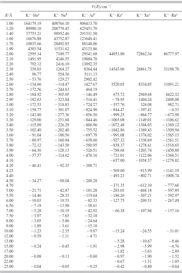
TABLE I. CCSD共T兲potentials for K⫹•He, K⫹•Ne, and K⫹•Ar. Energies are given with respect to the relevant dissociation limit.
R/Å
V(R)/cm⫺1
K⫹•Hea K⫹•Neb K⫹•Arb K⫹•Krc K⫹•Xec K⫹•Rnc
1.00 164179.19 408766.10 806413.70 1.20 80980.10 208778.45 425451.70 1.40 37753.21 98952.46 291531.50 1.60 16676.88 43752.87 123648.41 1.70 10835.66 28492.85 88148.06 1.90 4303.54 11531.62 43133.86
2.00 2595.14 7109.77 29541.68 44953.80 72862.34 86777.97 2.10 1491.95 4246.55 19884.70
2.20 792.12 2416.10 13092.35
2.30 358.03 1264.27 8364.44 14543.06 26861.75 33188.78 2.40 96.77 554.36 5111.13
2.50 ⫺53.76 129.27 2902.42
2.60 ⫺134.60 ⫺114.47 1427.67 3520.05 8334.05 11091.21 2.70 ⫺172.56 ⫺244.63 464.19
2.80 ⫺184.92 ⫺305.05 ⫺146.49 675.72 2969.68 4422.32 2.90 ⫺182.63 ⫺323.84 ⫺516.41 ⫺78.95 1404.24 2408.08 3.00 ⫺172.53 ⫺318.83 ⫺724.27 ⫺557.76 326.08 982.71 3.10 ⫺158.77 ⫺301.07 ⫺824.90 ⫺844.47 ⫺397.41 ⫺6.33 3.20 ⫺143.80 ⫺277.36 ⫺856.30 ⫺999.25 ⫺864.77 ⫺673.98 3.30 ⫺129.00 ⫺251.68 ⫺844.46 ⫺1065.08 ⫺1149.01 ⫺1106.62 3.40 ⫺115.09 ⫺226.29 ⫺806.96 ⫺1072.48 ⫺1304.05 ⫺1369.12 3.50 ⫺102.40 ⫺202.40 ⫺755.52 ⫺1042.86 ⫺1369.43 ⫺1509.94 3.60 ⫺91.04 ⫺180.56 ⫺697.78 ⫺991.08 ⫺1374.02 ⫺1565.15 3.70 ⫺80.97 ⫺160.94 ⫺638.60 ⫺927.32 ⫺1338.69 ⫺1561.51 3.80 ⫺72.12 ⫺143.50 ⫺580.95 ⫺858.37 ⫺1278.41 ⫺1518.65 3.90 ⫺64.36 ⫺128.13 ⫺526.51 ⫺788.68 ⫺1203.74 ⫺1450.88 4.00 ⫺57.57 ⫺114.62 ⫺476.16 ⫺721.01 ⫺1122.06 ⫺1368.51 4.10 ⫺657.00 ⫺1038.37 ⫺1278.82 4.20 ⫺46.41 ⫺92.35 ⫺388.71
4.25 ⫺569.60 ⫺915.99 ⫺1141.19 4.40 ⫺493.23 ⫺802.71 ⫺1008.74 4.50 ⫺34.27 ⫺68.04 ⫺288.28
4.70 ⫺371.35 ⫺612.10 ⫺777.66 5.00 ⫺21.71 ⫺42.87 ⫺181.28 ⫺283.03 ⫺468.18 ⫺597.89 5.50 ⫺14.46 ⫺28.35 ⫺119.64 ⫺186.26 ⫺307.21 ⫺392.97 6.00 ⫺10.03 ⫺19.53 ⫺82.33 ⫺127.75 ⫺209.51 ⫺267.49 6.50 ⫺7.18 ⫺13.90 ⫺58.61
7.00 ⫺5.28 ⫺10.19 ⫺42.92 ⫺66.38 ⫺107.94 ⫺137.16 7.50 ⫺3.97 ⫺7.65 ⫺32.18
8.00 ⫺3.05 ⫺5.86 ⫺24.64 9.00 ⫺1.89 ⫺3.61 ⫺15.18
10.00 ⫺1.23 ⫺2.35 ⫺9.87 ⫺15.24 ⫺24.55 ⫺31.01 12.00 ⫺0.59 ⫺1.11 ⫺4.71
13.00 ⫺5.28 ⫺10.67 ⫺8.46
15.00 ⫺0.24 ⫺0.45 ⫺1.91 ⫺2.98 ⫺5.99 ⫺4.76
17.00 ⫺1.82 ⫺3.63 ⫺2.89
20.00 ⫺0.08 ⫺0.13 ⫺0.60 ⫺0.97 ⫺1.90 ⫺1.52
22.00 ⫺0.67 ⫺1.31 ⫺1.05
25.00 ⫺0.04 ⫺0.05 ⫺0.25 ⫺0.42 ⫺0.80 ⫺0.64
the conclusion that the binding energy was not in error by more than 0.4%. In a follow-up paper,28 that potential was modified in order to fit mobility measurements better. It was concluded that, over the range of the potential tested by the mobility measurements, unexplained discrepancies of ⬃1% still existed between experiment and theory. Finally, Skullerud, Løvaas, and Tsurugida29 constructed a model po-tential with adjustable parameters, based on well-known ana-lytic forms23of the short and long-range regions of M⫹•Rg potentials; by fitting to the previous ab initio values of Ref. 28. The most accurate potential of these has been concluded29 to be the modified version of the EGF potential.28
We calculated potential energy curves over a wide range of R for the three sets of basis sets: aVQZ, aV5Z, and d-aV5Z. From these curves, we calculated rovibrational en-ergy levels, and used these to extract spectroscopic constants. The values are shown in Table II, and the potential energy curve is shown in Fig. 1. As may be seen from Table II, there is, on the whole, reasonable agreement between the three basis sets, with the difference between aV5Z and d-aV5Z being extremely small. There is a significant difference both in Deandeon going from aVQZ to aV5Z, suggesting that the shape of the curve changes between these two basis sets; the changes between the aV5Z and d-aV5Z levels of theory are very much smaller. Our best values for De and Re are 185.4 cm⫺1and 2.825 Å.
In Table III, we present the whole set of bound rovibra-tional levels obtained from our potential. Note that we obtain 53 bound rovibrational levels, whereas the SAPT potential of Moszynski26 only led to 36: this is likely a consequence of an incomplete description of electron correlation effects in
that work, leading to a shallower potential and fewer bound levels. As noted above, comparison with mobility data in Refs. 28 and 29 has led to the conclusion that the mobility-modified potential of Ref. 28 is very accurate, and so we compare to that potential also. Plots of that potential and our CCSD共T兲/d-aug-cc-pV5Z one lead to the conclusion that these are, indeed, very similar, with only very small differ-ences observable by eye. The modified EFG potential given in Ref. 28 leads to values of De⫽185.5 cm⫺1, and Re ⫽2.83 Å—both in very good agreement with the values ob-tained herein.
Vibrational energy levels and rotational constants are given in Table IV for the lowest few levels. Our best value for e is 100.4 cm⫺
1
[image:4.612.51.300.63.327.2], which compares favorably with the value of 101.4 cm⫺1 obtained from the mobility-modified potential. The value of 94.4 cm⫺1from the SAPT potential26 is not in such good agreement.
TABLE II. Calculated spectroscopic parameters for39K⫹•Rg.a
Species Re/Å e/cm⫺1 exe/cm⫺1 De/cm⫺1 Ref.
K⫹•4He 2.91 164 25 2.87 94.4b 14.6b 171 26
2.85 177.4 27
2.83b 101.4c 15.5c 185.5b 28 2.818 97.2 14.9 177.8 This work共aVQZ兲 2.825 100.2 15.2 184.1 This work共aV5Z兲 2.825 100.4 15.2 185.4 This work共d-aV5Z兲 K⫹•20Ne 2.97 314 25
2.87 350 29
2.940 69.0 4.50 311.9 This work共aVQZ兲 2.921 72.0 4.82 324.3 This work共aV5Z兲 K⫹•40Ar 3.13 938 25
3.11 990 29
3.42 490 30
3.225 80.6 2.36 829.8 This work共aVQZ兲 3.215 82.1 2.36 856.8 This work共aV5Z兲 K⫹•84Kr 3.30 1135 25
3.28 1157 29
3.356 74.1 1.51 1075.0 This work K⫹•132Xe 3.35 1721 25
3.46 1510 29
3.558 72.9 1.12 1378.0 This work K⫹•222Rn 3.641 71.0 0.93 1569.5 This work
aSee text for details.
bPotential of Ref. 26 analyzed in the present work. cPotential of Ref. 28 analyzed in the present work.
FIG. 1. Potential energy curves for the six K⫹•Rg species calculated at the CCSD共T兲level of theory. Basis sets used: d-aV5Z (K⫹•He); aV5Z (K⫹ •Ne and K⫹•Ar), and ECP basis sets for K⫹•Kr–K⫹•Rn. See text for details.
TABLE III. Energies of the bound rovibrational states (v,J) of 39K⫹•4He共cm⫺1). Relative to the dissociation limit (De⫽185.393 cm⫺1). Calculations performed at the CCSD共T兲/d-aug-cc-pV5Z level of theory.
J
v
0 1 2 3 4 5
0 ⫺136.930 ⫺66.873 ⫺27.203 ⫺8.630 ⫺1.781 ⫺0.136 1 ⫺135.864 ⫺66.018 ⫺26.583 ⫺8.239 ⫺1.584 ⫺0.079 2 ⫺133.733 ⫺64.313 ⫺25.349 ⫺7.466 ⫺1.206
3 ⫺130.542 ⫺61.765 ⫺23.515 ⫺6.333 ⫺0.682 4 ⫺126.297 ⫺58.385 ⫺21.100 ⫺4.874 ⫺0.081 5 ⫺121.008 ⫺54.190 ⫺18.133 ⫺3.142
6 ⫺114.687 ⫺49.199 ⫺14.655 ⫺1.221 7 ⫺107.346 ⫺43.441 ⫺10.719
8 ⫺99.004 ⫺36.948 ⫺6.401
9 ⫺89.680 ⫺29.763 ⫺1.813
10 ⫺79.400 ⫺21.941 11 ⫺68.193 ⫺13.553
12 ⫺56.092 ⫺4.699
13 ⫺43.140
14 ⫺29.387
[image:4.612.317.560.555.758.2]We conclude that, on the basis of the spectroscopic con-stants, there is little difference between the mobility-modified potential of Ref. 28, and the best potential obtained herein—we shall compare these potentials further when con-sidering the calculated transport constants below.
2. K¿"Ne
There has not been much work performed on K⫹•Ne. Ahlrichs et al.23 derived a model potential for the system, and this was modified in the later work by Skullerud et al.,29 where two adjustable parameters were used to fit the poten-tial to mobility data—this is denoted the SLT potenpoten-tial here-after. In addition, KMV共Ref. 25兲 also derived a model po-tential based upon a universal scaling procedure, again fitting to available mobility data. The two mobility-fitted potential energy curves25,29give good agreement with each other, with Ref. 25 obtaining Re⫽2.97 Å and De⫽314 cm⫺1, and Ref. 29 obtaining corresponding values of 2.87 Å and 350 cm⫺1. Again, in the present work, a wide range of R was used to calculate the potential for this species using both the aVQZ and aV5Z basis sets, andLEVELemployed to obtain spectro-scopic constants. The curve is shown in Fig. 1. As may be seen from Table II, reasonable agreement is obtained be-tween the CCSD共T兲/aVQZ and CCSD共T兲/aV5Z calculations, with the larger basis set giving Re⫽2.92 Å and De
⫽312 cm⫺1. These values are in good agreement with the potential energy curves obtained from fits to mobility data.25,29
Vibrational energy levels and rotational constants are given in Table IV for the lowest few levels.
3. K¿"Ar
Ahlrichs et al.23 used a model potential to describe the K⫹/Ar system. This potential was modified by Skullerud and co-workers29 with parameters fitted to mobility data; they obtained a potential with Re⫽3.13 Å and De⫽938 cm⫺1. The earlier potential of KMV,25 also obtained by fitting to available mobility data, had Re⫽3.11 Å and De ⫽990 cm⫺1. In addition, Bauschlicher et al.30 employed the modified coupled-pair functional 共MCPF兲 approach, with large basis sets, to obtain Re⫽3.42 Å and a dissociation en-ergy of 490 cm⫺1, which seems to be very low.
It is worth noting in passing that scattering cross sections obtained from molecular beam studies have been used to derive information about the K⫹•Rg systems. Powers and Cross31fitted their data to model potentials, obtaining a De value of 758 cm⫺1and an Revalue of 3.49 Å, clearly out of line with the mobility studies. Perhaps this is not too surpris-ing as such studies tend to be probsurpris-ing the repulsive region of the potential and, as noted in Ref. 6, these studies were un-able to gain any information on the lighter species, K⫹•He and K⫹•Ne, presumably since the potential was too shallow. The results from the present work are given in Table II, with the potential curve being presented in Fig. 1. As may be seen, the difference between the results using the CCSD共T兲/ aVQZ and the CCSD共T兲/aV5Z levels of theory is relatively small. Our best values are De⫽856.8 cm⫺1 and Re ⫽3.215 Å. The dissociation energy is similar to that obtained in the mobility studies,25,29 but is far removed from the MCPF value30 共see Table II兲. The value for e reported in Ref. 30 of 66 cm⫺1is also rather low compared to our best value of 82 cm⫺1.
Vibrational energy levels and rotational constants are given in Table IV for the lowest few levels.
4. K¿"Kr
For this species, there are only two sources of potentials to the authors’ knowledge. The first is Ref. 25 where poten-tials are reported, which 共as noted above兲were obtained by fitting to available mobility data. The second, more recent, one is that of Skullerud and co-workers,29who again used a model potential with parameters fitted to further mobility data. For K⫹•Kr, the KMV potential yielded Re⫽3.30 Å and
De⫽1135 cm⫺1, while the Skullerud potential gave corre-sponding values of 3.28 Å and 1157 cm⫺1. These values compare favourably to those obtained herein: De ⫽1075 cm⫺1 and Re⫽3.36 Å. In addition, we note that Powers and Cross31 obtained values of De⫽686 cm⫺1 and
[image:5.612.51.295.64.424.2]Re⫽3.59 Å from beam studies, and again these values seem to indicate a potential that is too shallow.
TABLE IV. Calculated rovibrational spectroscopic constants for39K⫹•Rg.a
v E(v,0)⫺E(0,0) Bv/cm⫺1 Dv/cm⫺1
K⫹•4He
0 0 0.533 8.953⫻10⫺5
1 70.06 0.427 15.29⫻10⫺5
2 109.73 0.310 25.94⫻10⫺5
3 128.30 0.197 40.87⫻10⫺5
K⫹•20Ne
0 0 0.145 2.81⫻10⫺6
1 62.36 0.135 3.43⫻10⫺6
2 115.08 0.125 4.23⫻10⫺6
3 158.69 0.114 5.24⫻10⫺6
K⫹•40Ar
0 0 8.15⫻10⫺2 3.49⫻10⫺7
1 77.35 7.93⫻10⫺2 3.74⫻10⫺7
2 149.99 7.70⫻10⫺2 4.04⫻10⫺7 3 217.97 7.46⫻10⫺2 4.37⫻10⫺7
K⫹•84Kr
0 0 5.54⫻10⫺2 1.31⫻10⫺7
1 70.90 5.43⫻10⫺2 1.38⫻10⫺7
2 138.78 5.32⫻10⫺2 1.46⫻10⫺7
3 203.66 5.21⫻10⫺2 1.54⫻10⫺7
K⫹•132Xe
0 0 4.40⫻10⫺2 6.66⫻10⫺8
1 70.67 4.33⫻10⫺2 6.90⫻10⫺8
2 139.09 4.26⫻10⫺2 7.16⫻10⫺8
3 205.27 4.19⫻10⫺2 7.44⫻10⫺8
K⫹•222Rn
0 0 3.81⫻10⫺2 4.55⫻10⫺8 1 69.16 3.76⫻10⫺2 4.68⫻10⫺8 2 136.47 3.71⫻10⫺2 4.83⫻10⫺8 3 201.93 3.66⫻10⫺2 5.00⫻10⫺8
aE(v,J)⫽E(v,0)⫹B
5. K¿"Xe
For K⫹•Xe, the KMV potential25 yielded Re⫽3.35 Å and De⫽1721 cm⫺1, while the corresponding values from the Skullerud et al. potential29were 3.46 Å and 1510 cm⫺1. These values are in reasonable agreement with the values of
De⫽1378 cm⫺1 and Re⫽3.56 Å obtained herein, but both appear to be a little deeper and more strongly bound than the present potentials, which are shown in Fig. 1. Again, the molecular beam studies yield a potential which seem to be too shallow, with De⫽1210 cm⫺1 and Re⫽4.00 Å.
We also note the study of Freitag et al.32 who used the coupled-electron-pair approximation 共CEPA兲method to cal-culate properties of M⫹•Xe species. They obtained values of: Re⫽3.77 Å, De⫽900 cm⫺1, e⫽57 cm⫺1, and exe ⫽1.0 cm⫺1. As may be seen, by comparison both with the previous mobility potentials and the values obtained herein
共Table II兲, Freitag et al.’s potential is also too shallow. Vibrational energy levels and rotational constants are given in Table IV for the lowest few levels.
6. K¿"Rn
There have been no previous studies on the K⫹•Rn sys-tems, and so the spectroscopic values presented in Tables II and IV constitute the only ones available; the potential en-ergy curve is given in Fig. 1. Our values are: De ⫽1570 cm⫺1, Re⫽3.64 Å, ande⫽71 cm⫺1.
7. Rovibrational data for the K¿"Rg species
In Table IV are given the energies of the lowest few pure vibrational levels, and it is from these levels that theeand exevalues in Table II are derived. One can see from Table II that the vibrational energies do not follow a monotonic trend with increasing molar mass: this may be understood by noting that there are two counteracting factors that are affect-ing the frequencies. First, as the mass of Rg increases, then the vibrational frequency would be expected to fall, all things being equal; but secondly, as Rg increases in size it becomes more polarizable, and so the interaction energy is expected to increase 共as observed兲, which is expected to in-crease the frequency. These two effects are in competition and lead to the observed oscillation in the frequency. It is also seen that the anharmonicity of the vibration decreases as Rg increases in size: this is to be expected as the well-depth increases.
B. Transport properties
There have been many studies of the transport of K⫹in rare gases, with all gases having been studied except radon. For helium and argon in particular, the number of studies is quite large, covering a variety of transport coefficients over wide ranges of E/N, and at a variety of temperatures. For this reason, and as was the case for Li⫹ and Na⫹ 共Refs. 5 and 6兲we have placed the results in the gaseous ion transport database at Chatham College.33
The differences between the measured and calculated transport coefficients are compared using statistical quanti-ties,␦and, which take into account the estimated errors in each quantity.22 In order to compare the data informatively,
some idea of the meanings of ␦ and is required. If the experimental and calculated errors are the same at all E/N, then␦is the ratio of the average percentage difference to the maximum combined percentage difference expected, while is the ratio of the standard deviation of the percentage differ-ences to the root mean square of the maximum combined percentage deviations expected. A positive value of ␦ indi-cates that the data lie above the calculated values, and vice versa. Values of兩␦兩that are substantially lower共alternatively, higher兲 than 1 indicate that there is substantial agreement
共disagreement兲between the calculated and measured values, on average. Values of that are not much larger than 兩␦兩 indicate that there is little scatter in the experimental data and that the agreement between the calculated and measured values is uniform over all values of E/N, while values of substantially greater than兩␦兩indicate that at least one of these factors is not true. The statistical comparisons are performed at low, intermediate and high E/N regions.
[image:6.612.332.541.49.325.2]1. K¿ in He
The experimental data has been reported in Refs. 28, 35– 42, and our calculations are compared to those studies in Table V. The experimental studies cover a very wide range of temperature and E/N, providing a good set of data to which to compare the potential energy curves.
For all of the potentials, the D⬜/K data from Ref. 41 give␦values greater than 1 at low E/N, between⫺1 and⫹1 at intermediate E/N, and below ⫺1 at high E/N. We con-clude that these experimental data are significantly too high at low E/N, about right between 30 and 150 Td, and signifi-cantly too low at high E/N. In part, this conclusion comes from the high accuracy共2%兲claimed for these data, but pri-marily it points to a systematic error of unknown origin in the experiments.
With the possible exception of the KMV potential,25 none of the potentials match the diffusion data from Ref. 39 above 20 Td. This is consistent with recent experimental re-sults for other atomic ion-atom systems43 that indicate that the Georgia Tech data at high E/N suffer from a flawed method for extracting transport coefficients from the raw ar-rival time data. The flaw in the data analysis has a more serious impact on diffusion than on mobility, and so it is logical that disagreement begins at smaller E/N for the D储 data.
The 80 K data from Ref. 42 shows considerable scatter, as evinced by large values of , and they are poorly de-scribed by every potential studied, as indicated by␦ values substantially below⫺1, probably indicating that these values are not too reliable.
It was stated in 1991共Ref. 41兲that ‘‘none of the avail-able potentials is completely correct.’’ The only potential in-cluded here that was subject to this statement is the KMV one.25Indeed, this potential describes well the mobility data
from Ref. 38 that were used to determine its parameters, but it does not match the data obtained since 1991. The most logical reason for its poor agreement with the later data is that the mobility data in Ref. 38 is not as accurate as those for other systems; this is consistent with the fact that the ␦ values obtained for this system using other potentials are close to or slightly above the value of ⫹1 that indicates a significant disagreement. We conclude that the KMV poten-tial and the data from Ref. 38 are not reliable.
The potential curves from Refs. 26 and 27 are ab initio potentials that match the experimental data from Refs. 35– 37, 40, and 41 moderately well. However, the ␦ values are consistently negative for the potential from Ref. 26, while those for the potential from Ref. 27 are approximately evenly split between positive and negative values. This suggests that the latter potential is a more accurate representation of the true K⫹•He interaction potential than the former.
Only the potential from Ref. 28 and the current aV5Z and d-aV5Z potentials match the rest of the data with 兩␦兩 values⬍1 and withvalues smaller than 1. This is particu-larly striking for the mobility data from Ref. 28, which are not only the most recent data but also have the highest claimed accuracy. Given that the aVQZ potential is not suf-ficient to describe the mobility data, it suggests that the de-mands on basis set for these rather simple systems is quite stringent. It appears a quintuple- basis set is required— likely due to the weak nature of this interaction, caused by the low polarizability of the He atom.
In summary, the potential from Ref. 28 and the present CCSD共T兲/aV5Z and CCSD共T兲/d-aV5Z potentials are the best available for this system. Only the present potentials are
ab initio potentials. Although most of the experimental data
[image:7.612.52.561.65.310.2]does not distinguish between these two potentials, the recent data from Ref. 28 is matched marginally better by the
TABLE V. Statistical comparison of calculated and experimental transport data for K⫹ions in He gas.a
Data type Range of E/N A No.
Potential source
Ref. 25 Ref. 29
This work
aVQZ aV5Z d-aV5Z
P ␦ P ␦ P ␦ P ␦ P ␦
K0
303 K Ref. 37
9–20 2 14 0.1 ⫺1.150 1.160 0.4 ⫺0.729 0.751 0.1 ⫺0.236 0.279 0.1 0.001 0.146 0.1 0.128 0.195 20– 82 2 18 0.1 ⫺0.765 0.801 0.4 0.143 0.412 0.1 0.080 0.242 0.1 0.093 0.200 0.1 0.143 0.217 9– 82 32 ⫺0.93 0.98 ⫺0.24 0.59 ⫺0.06 0.26 0.05 0.18 0.14 0.21
K0
76.8 K Ref. 28
2–15 0.5 11 0.1 ⫺3.342 3.573 0.4 ⫺3.198 3.335 0.1 ⫺0.773 1.075 0.1 0.373 0.630 0.1 0.590 0.682
K0
294 K Ref. 28
2–19 0.5 9 0.1 ⫺5.114 5.118 0.4 ⫺3.178 3.183 0.1 ⫺1.837 1.850 0.1 ⫺0.780 0.828 0.1 ⫺0.275 0.405 19–35 0.5 4 0.1 ⫺4.155 4.182 0.4 ⫺1.329 1.453 0.1 ⫺1.240 1.291 0.1 ⫺0.837 0.858 0.1 ⫺0.539 0.559 2–35 13 ⫺4.82 4.85 ⫺2.61 2.77 ⫺1.65 1.70 ⫺0.80 0.84 ⫺0.36 0.46
K0
295 K Ref. 28
2–29 0.5 10 0.1 ⫺4.998 5.020 0.4 ⫺2.889 2.977 0.1 ⫺1.773 1.811 0.1 ⫺0.827 0.847 0.1 ⫺0.353 0.379 29–51 0.5 4 0.1 ⫺3.012 3.024 0.4 ⫺0.031 0.478 0.1 ⫺0.208 0.324 0.1 ⫺0.118 0.159 0.1 0.074 0.097 51–300 0.5 13 0.1 ⫺3.822 3.963 0.4 2.070 2.148 0.1 1.389 1.477 0.1 0.948 1.034 0.1 0.953 1.031 2–300 27 ⫺4.14 4.27 ⫺0.08 2.35 ⫺0.02 1.51 0.13 0.89 0.34 0.75
D⬜/K 294 K Ref. 28
4 –19 3 6 0.3 ⫺0.058 0.317 1 0.087 0.269 1 0.111 0.292 1 0.063 0.286 1 0.080 0.295 19–75 3 8 0.3 ⫺0.797 0.902 1 0.557 0.705 1 ⫺0.054 0.371 1 ⫺0.265 0.429 1 ⫺0.299 0.444 75–220 3 8 0.3 ⫺2.310 2.447 1 0.823 1.009 1 0.424 0.504 1 0.221 0.347 1 0.196 0.327 4 –220 22 ⫺1.15 1.58 0.53 0.76 0.16 0.41 0.00 0.36 ⫺0.02 0.37
a
CCSD共T兲/d-aV5Z potential. Hence, this ab initio potential appears to be the best potential available for this system, but the differences between it, the CCSD共T兲/aV5Z one, and that of Ref. 28 are very small.
2. K¿ in Ne
The experimental work on K⫹in Ne has been published in Refs. 29, 35–39. Again, the experimental studies cover a very wide range of temperatures and E/N, providing a good set of data to which to compare the potential energy curves. The comparison between the calculated transport data and the experimental is presented in Table VI.
All of the potentials match the available data except for the diffusion data39 at high E/N from the Georgia Tech group. Again, this is consistent with a flawed method for extracting transport coefficients 共see discussion above for K⫹•He). The present ab initio potentials are at least as good, and are perhaps slightly better, at matching the data than are the two model potentials from Refs. 25 and 29, although this is not conclusive. The SLT model potential29 does the best job of fitting the data reported in the same paper, but that is natural since the potential parameters were fitted to that data. The fit of the present potentials to these recent data is accept-able. It is not conclusive whether the aVQZ or the aV5Z
potentials of the present work perform better at describing the transport data or not; with each potential fitting some data better than the other. This inconclusiveness is due to the closeness of the two potentials.
3. K¿ in Ar
The experimental work on K⫹in Ar has been published in Refs. 35–37, 41, 44 – 48. Again, a fairly wide range of
E/N and temperatures has been covered. Comparison of the
calculated data with the experimental is given in Table VII, from which we make the following comments.
[image:8.612.49.570.64.211.2]In 1991, Hogan and Ong49 concluded that the KMV potential25 was the best one available at that time, in the sense that it did the best job of matching the experimental transport data. However, this potential is in significant or nearly significant disagreement with all of the data except that from Ref. 36, which was the data used to determine the parameter values for that model potential. We conclude that the mobility data from Ref. 36 is inaccurate and that the KMV potential for this system should no longer be consid-ered reliable. The SLT model potential29and the aVQZ and aV5Z potentials from the present work do not agree well with the experimental mobilities from Ref. 35, whether at
TABLE VI. Statistical comparison of calculated and experimental transport data for K⫹ions in Ne gas.a
Data type
Range of
E/N A
No. of points
Potential source
Ref. 25 Ref. 29
This work
aVQZ aV5Z
P ␦ P ␦ P ␦ P ␦
K0
302 K Ref. 37
9–25 2 10 0.1 ⫺0.017 0.089 1 0.423 0.428 0.1 ⫺0.304 0.315 0.1 0.045 0.097 25– 81 2 16 0.1 0.057 0.152 1 0.231 0.290 0.1 0.158 0.220 0.1 0.243 0.266 9– 81 26 0.03 0.13 0.30 0.35 ⫺0.02 0.26 0.16 0.22
D⬜/K 295 K Ref. 29
4 –25 1 8 1 ⫺0.427 0.504 1 ⫺0.089 0.240 1 ⫺0.468 0.546 1 ⫺0.384 0.448 25–70 1 7 1 ⫺1.013 1.023 1 ⫺0.347 0.417 1 ⫺0.625 0.667 1 ⫺0.560 0.587 70–350 1 9 1 ⫺2.778 2.954 1 ⫺0.719 0.740 1 ⫺0.573 0.612 1 ⫺0.743 0.772 4 –350 24 ⫺1.42 1.86 ⫺0.40 0.52 ⫺0.55 0.61 ⫺0.57 0.63
aA⫽accuracy of experiment共%兲. P⫽precision of calculations共%兲.
TABLE VII. Statistical comparison of calculated and experimental transport data for K⫹ions in Ar gas.a
Data type Range of E/N A No. of points
Potential source
Ref. 25 Ref. 29
This work
aVQZ aV5Z
P ␦ P ␦ P ␦ P ␦
K0304 K
Ref. 37
9– 46 2 17 0.1 0.995 1.011 0.1 0.567 0.580 0.1 ⫺0.341 0.359 0.1 0.160 0.180 46 –110 2 15 0.3 1.220 1.259 0.3 1.959 2.034 0.3 0.177 0.446 0.3 0.679 0.779 9–110 32 1.10 1.13 1.22 1.46 ⫺0.10 0.40 0.40 0.55
K0295 K
Ref. 42
3– 46 0.5 14 0.1 1.683 1.726 0.1 0.479 0.505 0.1 ⫺2.178 2.272 0.1 ⫺0.596 0.695 46 –120 0.5 8 0.3 3.530 3.667 0.3 3.806 4.052 0.3 ⫺0.539 1.240 0.3 2.006 2.390 3–120 22 2.35 2.60 1.69 2.48 ⫺1.58 1.96 0.45 1.61
D⬜/K 298 K Ref. 48
10– 46 3 8 1 0.425 0.624 2 0.184 0.359 1 ⫺0.061 0.404 1 0.068 0.363 46 –185 3 10 3 ⫺0.698 0.879 5 ⫺0.283 0.401 3 ⫺0.595 0.664 3 ⫺0.415 0.499 185– 600 3 16 1 ⫺2.599 2.614 1 ⫺0.555 0.602 1 ⫺0.770 0.805 1 ⫺0.770 0.834 10– 600 32 ⫺1.41 1.94 ⫺0.32 0.51 ⫺0.59 0.71 ⫺0.469 0.657
[image:8.612.50.566.572.749.2]197 K or 275 K. Given the remaining comments, we con-clude that the experimental data are high by more than the 2% accuracy claimed for them.
The aVQZ potential matches the mobility data from Ref. 44 quite well, much better than the SLT model potential29or indeed the aV5Z one. None of the potentials matches the parallel diffusion coefficient data at intermediate or high
E/N, indicating that the diffusion data 共unlike the mobility data兲is not as accurate as claimed.
The aVQZ potential matches the mobility data from Ref. 45 quite well at low and intermediate E/N—much better than does the potential of Ref. 29 or the aV5Z one. The perpendicular diffusion data from Ref. 45 is adequately re-produced by all three potentials. Nevertheless, the calculated mobilities at high E/N are not adequately represented by the potentials, suggesting that the experimental values at high
E/N are high by more than the 1.5% accuracy claimed for
them.
The SLT model potential29reproduces the mobility data from Ref. 36 with extraordinarily high precision at all E/N, whereas the current aVQZ and aV5Z potentials only repro-duce them with moderate success. However, this situation is reversed for the mobility data from Ref. 37, making defini-tive conclusions difficult.
The mobility data from Ref. 46 is not well represented by the SLT model potential29 or the two current potentials, probably partly because the temperature varied substantially during the experiments, as noted therein.
The SLT model potential29reproduces the mobility data from Ref. 47 with good precision at all E/N, much better than any other potential. The agreement is particularly strik-ing at low E/N. However, the parallel diffusion data from the same work is not well described by any of the potentials, suggesting that it is too high by more than the 5% accuracy claimed. It is also the case that the mobility data from Ref. 42 is not well represented by the SLT model potential29 or the two current potentials.
The SLT model potentials29 and the present aVQZ and aV5Z potentials represent the D⬜/K data from Ref. 48 quite well, which attests to their reliability since the accuracy claimed for these data is very good共3%兲.
An overall assessment of these results, particularly the comparison with the results from Refs. 36 and 48, suggests
that the SLT model potential29 and the present aVQZ poten-tial are of approximately equal reliability and that the avail-able experimental data do not clearly indicate which of the two potentials is likely to be closer to the true interaction potential for the K⫹•Ar system. Interestingly, the preponder-ance of the data suggest that the aV5Z potential is in slightly poorer agreement with the experimental data than is the aVQZ one—this is surprising since the larger basis set would be expected to be more reliable. Possible interpretations are that the aVQZ potential benefits from a cancellation of er-rors, or that the experimental data are not as accurate as claimed so that the statistics are leading to an incorrect con-clusion. Only further experimental work will unravel this question.
4. K¿ in Kr
The experimental data has been reported in Refs. 29, 41, 50, and 51.共Note that the data in Ref. 41 have been adjusted to 298 K.兲The statistics describing the comparison between the calculated data and the experimental is given in Table VIII. From these statistics it can be concluded that the KMV potential25 only fits the mobility data from Ref. 51, i.e., the data from which the fitted parameters were derived. Given that this potential does not fit the diffusion data in Ref. 51, which was obtained by the same group, then the KMV potential25must be considered unreliable.
The SLT model potential29and the present potential de-scribe the complete set of experimental data with about the same reliability, although the SLT potential describes the mo-bility and diffusion data from the Georgia Tech group slightly better. Given the comments in the previous para-graph, it is likely that at least the diffusion data are actually of a lower accuracy than was claimed.
The present potential fits both sets of D⬜/K data better than does the SLT model potential. Overall, there is an indi-cation that the present potential is slightly more accurate than is the SLT one; however it is not conclusive.
5. K¿ in Xe
[image:9.612.52.563.64.204.2]The experimental data has been reported in Refs. 29, 50, and 51, and the statistics describing the comparison between the calculated data and the experimental is given in Table IX.
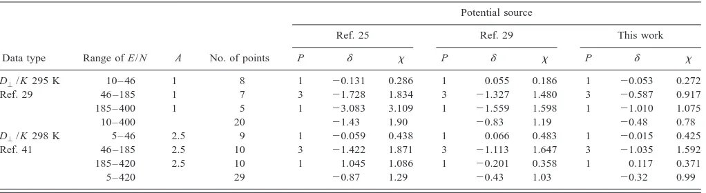
TABLE VIII. Statistical comparison of calculated and experimental transport data for K⫹ions in Kr gas.a
Data type Range of E/N A No. of points
Potential source
Ref. 25 Ref. 29 This work
P ␦ P ␦ P ␦
D⬜/K 295 K Ref. 29
10– 46 1 8 1 ⫺0.131 0.286 1 0.055 0.186 1 ⫺0.053 0.272 46 –185 1 7 3 ⫺1.728 1.834 3 ⫺1.327 1.480 3 ⫺0.587 0.917 185– 400 1 5 1 ⫺3.083 3.109 1 ⫺1.559 1.598 1 ⫺1.010 1.075 10– 400 20 ⫺1.43 1.90 ⫺0.83 1.19 ⫺0.48 0.78
D⬜/K 298 K Ref. 41
5– 46 2.5 9 1 ⫺0.059 0.438 1 0.066 0.483 1 ⫺0.015 0.425 46 –185 2.5 10 3 ⫺1.422 1.871 3 ⫺1.113 1.647 3 ⫺1.035 1.592 185– 420 2.5 10 1 1.045 1.086 1 ⫺0.201 0.358 1 0.117 0.371 5– 420 29 ⫺0.87 1.29 ⫺0.43 1.03 ⫺0.32 0.99
The KMV potential25 is found not to fit any of the ex-perimental data very well; interestingly, not even the data from which the fitted parameters were obtained.50 The SLT model potential and the present ab initio potential both fit the available data with about the same reliability, suggesting that both of these potentials are about as accurate as each other in describing the K⫹•Xe interaction.
6. K¿ in Rn
Since there is no experimental data, nor any previous theoretical work, then no comparison for this system can be made. An example of the calculated data is, however, pre-sented in Fig. 2.
IV. CONCLUSIONS
Both the calculated spectroscopic data and transport data point to the present ab initio potentials being extremely ac-curate. It is important to note that the potentials calculated here, the spectroscopic parameters and the transport data are all ab initio and consequently have no adjustable parameters anywhere. The excellent agreement with the model potentials of Skullerud et al.,29 which were based on a simple model potential with parameters fitted to accurate mobility data, and the present potentials indicate that truly reliable potentials are available for the K⫹•He–K⫹•Rn species. Interestingly, there was not always a clear indication that the aV5Z basis set was performing better than the smaller aVQZ ones for K⫹•He–K⫹•Ar; indeed, sometimes the indications were that the performance was the opposite to expectations. The only reasonable conclusion to draw from this is that this is an artifact caused by the statistical analysis, which builds in the accuracy of the experimental data. Although it might be ar-gued that better experiments might be able to spread some light on this matter, many of the experiments are already extremely accurate. We do note that we have used a combi-nation of all-electron and ECP-based basis sets, and that con-sequently, there is some inconsistency in the treatment of core-correlation effects and the inclusion of relativistic ef-fects; however, the large valence basis sets used in all cases ought to be able to describe the interactions here adequately. We were also able, based on the large body of data avail-able and a statistical analysis, to make conclusions as to the reliability of the different sets of diffusion and mobility data, and also to make similar comments regarding potentials.
In conclusion, in this work we have calculated very ac-curate ab initio potentials for the set of six K⫹•Rg species, and have shown that these are able to reproduce even very accurate transport data.
ACKNOWLEDGMENTS
The authors are grateful to the EPSRC for the award of computer time at the Rutherford Appleton Laboratories un-der the auspices of the Computational Chemistry Working Party 共CCWP兲, which enabled these calculations to be per-formed, and for a studentship to J.L. E.P.F.L. is grateful to the Research Grant Council共RGC兲 of the Hong Kong Spe-cial Administration Region 共HKSAR兲 and the Research Committee of the Hong Kong Polytechnic University for support. P.S. would like to thank the EPSRC for his present funding at Durham 共Senior Research Assistantship兲. The work of L.A.V. was supported by the National Science Foun-dation.
1F. E. Budenholzer, J. J. Galante, E. A. Gislason, and A. D. Jorgensen,
Chem. Phys. Lett. 33, 245共1975兲.
2F. E. Budenholzer, E. A. Gislason, and A. D. Jorgensen, J. Chem. Phys.
78, 5279共1983兲.
3
L. A. Viehland and E. A. Mason, Ann. Phys.共N.Y.兲91, 499共1975兲.
4I. R. Gartland, L. A. Viehland, and E. A. Mason, J. Chem. Phys. 66, 537
共1977兲.
5J. Lozeille, E. Winata, P. Solda´n, E. P. F. Lee, L. A. Viehland, and T. G.
Wright, Phys. Chem. Chem. Phys. 4, 3601共2002兲.
6
L. A. Viehland, J. Lozeille, P. Solda´n, E. P. F. Lee, and T. G. Wright, J. Chem. Phys. 119, 3729共2003兲.
7D. Bellert and W. H. Breckenridge, Chem. Rev.共Washington, D.C.兲102,
1595共2002兲.
8
P. Solda´n, E. P. F. Lee, and T. G. Wright, Phys. Chem. Chem. Phys. 3, 4661共2001兲.
9J. J. Wood and A. M. Boring, Phys. Rev. B 18, 27016共1978兲. 10E. P. F. Lee and T. G. Wright, J. Phys. Chem. A 103, 7843共1999兲. 11
E. P. F. Lee, S. D. Gamblin, and T. G. Wright, Chem. Phys. Lett. 322, 377
共2000兲.
12E. P. F. Lee and T. G. Wright, Mol. Phys. 101, 405共2003兲.
13EMSL Basis Set Library. Basis sets were obtained from the Extensible
Computational Chemistry Environment Basis Set Database, Version 1/29/01, as developed and distributed by the Molecular Science Comput-ing Facility, Environmental and Molecular Sciences Laboratory which is part of the Pacific Northwest Laboratory, P.O. Box 999, Richland, Wash-ington 99352, USA, and funded by the U.S. Department of Energy. The Pacific Northwest Laboratory is a multi-program laboratory operated by Battelle Memorial Institute for the U.S. Department of Energy under Con-tract No. DE-AC06-76RLO 1830. Contact David Feller or Karen Schu-chardt for further information.
14E. P. F. Lee and T. G. Wright, Chem. Phys. Lett. 363, 139共2002兲. 15
T. Leininger, A. Nicklass, W. Ku¨chle, H. Stoll, M. Dolg, and A. Bergner, Chem. Phys. Lett. 255, 274共1996兲.
[image:10.612.50.566.64.163.2]16S. F. Boys and F. Bernardi, Mol. Phys. 19, 533共1970兲.
TABLE IX. Statistical comparison of calculated and experimental transport data for K⫹ions in Xe gas.a
Data type Range of E/N A No. of points
Potential source
Ref. 25 Ref. 29 This work
P ␦ P ␦ P ␦
D⬜/K 295 K Ref. 29
10–51 1 9 1 ⫺0.120 0.157 1 ⫺0.142 0.207 1 ⫺0.414 0.572 51–151 1 6 3 ⫺1.204 1.416 3 ⫺1.469 1.628 3 ⫺1.749 1.918 151– 400 1 5 1 ⫺3.480 3.505 1 ⫺1.110 1.131 1 ⫺0.571 0.613 10– 400 20 ⫺1.29 1.92 ⫺0.78 1.06 ⫺0.85 1.16
17
MOLPROis a package of ab initio programs written by H.-J. Werner, P. J. Knowles, with contributions from J. Almlo¨f, R. D. Amos, A. Berning
et al. The CCSD treatment is described in C. Hampel, K. Peterson, and
H. J. Werner, Chem. Phys. Lett. 190, 1共1992兲.
18P. Solda´n, E. P. F. Lee, and T. G. Wright, J. Chem. Soc., Faraday Trans. 94,
3307共1998兲.
19R. J. Le Roy,
LEVEL 7.2, A computer program for solving the radial Schro¨-dinger equation for bound and quasibound levels, and calculating various expectation values and matrix elements共University of Waterloo Chemical Physics Research Program Report CP-555R, 2000兲.
20L. A. Viehland, Comput. Phys. Commun. 142, 7共2001兲. 21L. A. Viehland, Chem. Phys. 70, 149共1982兲.
22
L. A. Viehland, Chem. Phys. 179, 71共1994兲.
23
R. Ahlrichs, H. J. Bohm, S. Brode, K. T. Tang, and J. P. Toennies, J. Chem. Phys. 88, 6290共1988兲.
24G. R. Ahmadi, J. Almlo¨f, and I. Røeggen, Chem. Phys. 119, 33共1995兲. 25A. D. Koutselos, E. A. Mason, and L. A. Viehland, J. Chem. Phys. 93,
7125共1990兲.
26R. Moszynski, B. Jeziorski, G. H. F. Diercksen, and L. A. Viehland, J.
Chem. Phys. 101, 4697共1994兲.
27I. Røeggen, H. R. Skullerud, and M. T. Elford, J. Phys. B 29, 1913共1996兲. 28
H. R. Skullerud, M. T. Elford, and I. Røeggen, J. Phys. B 29, 1925共1996兲.
29
H. R. Skullerud, T. H. Lovaas, and K. Tsurugida, J. Phys. B 32, 4509
共1999兲.
30C. W. Bauschlicher, Jr., H. Partridge, and S. R. Langhoff, J. Chem. Phys.
91, 4733共1989兲.
31
T. R. Powers and R. J. Cross, Jr., J. Chem. Phys. 58, 626共1973兲.
32A. Freitag, C. van Wu¨llen, and V. Staemmler, Chem. Phys. 192, 267
共1995兲.
33To access this database you must telnet to the computer named
sassafrass-.chatham.edu and log on as gastrans. The required password will be pro-vided upon request by email to viehland@sassafrass.chatham.edu.
34See EPAPS Document No. E-JCPSA6-120-310421 for extended versions
of Tables V–IX. A direct link to this document may be found in the online article’s HTML reference section. The document may also be reached via the EPAPS homepage 共http://www.aip.org/pubservs/epaps.html兲 or from
ftp.aip.org in the directory /epaps/. See the EPAPS homepage for more information.
35R. P. Creaser, Ph.D. thesis, Australian National University, 1969共
unpub-lished兲.
36H. B. Milloy and R. E. Robson, J. Phys. B 6, 1139共1973兲. 37R. P. Creaser, J. Phys. B 7, 529共1974兲.
38D. R. James, E. Graham, G. R. Akridge, and E. W. McDaniel, J. Chem.
Phys. 62, 740共1975兲.
39
D. R. James, E. Graham, G. R. Akridge, I. R. Gatland, and E. W. McDaniel, J. Chem. Phys. 62, 1702共1975兲.
40N. Takata, J. Phys. B 8, 2390共1975兲.
41M. J. Hogan and P. P. Ong, J. Chem. Phys. 95, 1973共1991兲. 42
R. A. Cassidy and M. T. Elford, 3rd International Swarm Seminar Pro-ceedings, Innsbruck, 1983, Aust. J. Phys. 39, 25共1986兲.
43T. H. Lovaas, H. R. Skullerud, O.-H. Kristensen, and D. Lihjell, J. Phys. D
20, 1465共1990兲.
44Technical Report, Georgia Tech., 1972, subsequently published in D. R.
James, E. Graham IV, G. M. Thomson, I. R. Gatland, and E. W. McDaniel, J. Chem. Phys. 58, 3652共1973兲.
45H. R. Skullerud, Technical Report No. EIP 72-3, University of Trondheim,
Norway, 1972.
46
N. Takata, J. Phys. B 10, 2749共1977兲. Data actually obtained at 295–311 K.
47M. Takebe, Y. Satoh, K. Iinuma, and K. Seto, J. Chem. Phys. 73, 4071
共1980兲.
48P. P. Ong and M. J. Hogan, J. Phys. B 24, 633共1991兲. 49
M. J. Hogan and P. P. Ong, Phys. Rev. A 44, 1597共1991兲.
50D. R. Lamm, M. G. Thackston, F. L. Eisele, H. W. Ellis, J. R. Twist, W. M.
Pope, I. R. Gatland, and E. W. McDaniel, J. Chem. Phys. 74, 3042共1981兲.
51W. M. Pope, F. L. Eisele, M. G. Thackston, and E. W. McDaniel, J. Chem.
Phys. 69, 3874共1978兲.
52
Smoothed data taken from H. W. Ellis, E. W. McDaniel, D. L. Albritton, L. A. Viehland, S. L. Lin, and E. A. Mason, At. Data Nucl. Data Tables 22, 179共1978兲.
53Smoothed data from H. W. Ellis, R. Y. Pai, E. W. McDaniel, E. A. Mason,