The effect of thermal conduction on the Virgo cluster

arXiv:astro-ph/0507443v1 19 Jul 2005

The Effects of Thermal Conduction on the ICM of the

Virgo Cluster

Edward C.D. Pope

_{, Georgi Pavlovski}

_{, Christian R. Kaiser}

_{, Hans Fangohr}

1_{School of Physics & Astronomy, University of Southampton, UK, SO17 1BJ} 2_{School of Engineering Sciences, University of Southampton, UK, SO17 1BJ}

5 February 2008

ABSTRACT

Thermal conduction has been suggested as a possible mechanism by which suffi-cient energy is supplied to the central regions of galaxy clusters to balance the effect of radiative cooling. Recent high resolution observations of the nearby Virgo cluster make it an ideal subject for an attempt to reproduce the properties of the cluster by numerical simulations, since most of the defining parameters are comparatively well known. Here we present the results of a simulated high-resolution, 3-d Virgo cluster for different values of thermal conductivity (1, 1/10, 1/100, 0 times the full Spitzer value). Starting from an initially isothermal cluster atmosphere we allow the cluster to evolve freely over timescales of roughly 1.3₋4.7_×109yrs. Our results show that

ther-mal conductivity at the Spitzer value can increase the central ICM radiative cooling time by a factor of roughly 3.6. In addition, for larger values of thermal conductvity the simulated temperature and density profiles match the observations significantly better than for the lower values. However, no physically meaningful value of thermal conductivity was able to postpone the cooling catastrophe (characterised by a rapid increase in the central density) for longer than a fraction of the Hubble time nor ex-plain the absence of a strong cooling flow in the Virgo cluster today. We also calculate the effective adiabatic index of the cluster gas for both simulation and observational data and compare the values with theoretical expectations. Using this method it ap-pears that the Virgo cluster is being heated in the cluster centre by a mechanism other than thermal conductivity. Based on this and our simulations it is also likely that the thermal conductvity is suppressed by a factor of at least 10 and probably more. Thus, we suggest that thermal conductvity, if present at all, has the effect of slowing down the evolution of the ICM, by radiative cooling, but only by a factor of a few.

Key words: thermal conduction-galaxies: clusters-individual(Virgo)-galaxies: active-cooling flows

1 INTRODUCTION

The strong central peak of the X-ray surface brightness profiles of many clusters of galaxies is generally inter-preted as the signature of a cooling flow (Cowie & McKee 1977; Fabian 1994). Standard cooling flow theory suggests that this peak should coincide with the deposition of large amounts of cold gas and significant excess of star forma-tion at the centre of the cooling flow. However, the XMM-Newton and Chandra satellites have demonstrated both the lack of the expected cold gas, at temperatures below roughly 1 keV (e.g. Edge 2001), and that spectroscopically mea-sured mass-deposition rates are roughly one tenth of the

⋆ _{E-mail:[email protected]}

value inferred from the peaks of cluster X-ray surface bright-ness maps (Voigt & Fabian 2004). These findings suggest that the gas in the cluster cores is reheated; either con-tinually or periodically, in order to produce the observed minimum central temperature (or entropy) and the lack of significant excess star formation. In recent years, work has concentrated on two main possibilities for heating the gas in the central regions of clusters: (1) heating by out-flows from AGN (e.g. Tabor & Binney 1993; Churazov et al. 2001; Br¨uggen & Kaiser 2002) and (2) transportation of heat from the outer regions of the cluster by thermal con-duction (e.g. Zakamska & Narayan 2003; Voigt et al. 2002; Voigt & Fabian 2004). In this paper we shall concentrate purely on thermal conduction.

centres of many relaxed clusters allows the possibility that thermal conduction may play a role in reducing the radiative energy losses in the cluster centre. Indeed, Zakamska & Narayan (2003) show that for several galaxy clusters the inward heatflow from the outer regions due to thermal conduction may be sufficient to balance the radia-tive losses although, in a different sample Voigt et al. (2002) show that thermal conduction is only able to balance radia-tive losses in the outer regions of the cluster core. However, though it is possible to achieve an energy balance for these clusters in their present state, this requires the thermal con-ductivity to vary as a function of radius. Furthermore, it is unclear what effect thermal conduction would have on the intra cluster medium (ICM) if it constitutes a significant process throughout the lifetime of the cluster. Since thermal conduction acts to oppose the formation of the temperature gradient that causes it, one might expect that the temper-ature and density profiles for those clusters in which ther-mal conduction plays a significant role to appear different compared to those clusters in which thermal conduction is less effective. In particular, the temperature profiles in such clusters could be much flatter than in clusters where thermal condcution is heavily suppressed. In addition, temperature gradients also occur outwards towards the edge of clusters. Therefore, it is possible that the high thermal conductivi-ties required to balance the radiative losses may also have a cooling effect by transporting energy away from the cluster centre and out into intercluster space (Loeb 2002).

One of the primary problems for studying the effects of thermal conduction in plasmas is the unknown value of the thermal conductivity. The theoretical value for the thermal conductivity of a fully ionized, unmagnetized plasma was originally calculated by Spitzer (1962). However, observa-tions indicate the existence of a magnetic field in the ICM (B<10µG; e.g. Carilli & Taylor 2002) which can affect this value dramatically. For magnetic fields of these strengths the electron and proton gyro radii are much smaller than their mean free paths along the field lines. The precise effect that magnetic fields have on thermal conductivity is unclear, al-though for magnetic fields of the observed strengths the ef-fective thermal conductivity is determined by the topology of the field (Markevitch et al. 2003). A magnetic field tan-gled on scales much longer than the electron mean free path will suppress thermal conduction perpendicular to the field lines reducing the thermal conductivity to at most one third of the full Spitzer value (if transport along the field line is unaltered) (Sarazin 1986). For a magnetic field tangled on scales shorter than the electron mean free path the conduc-tivity is suppressed by a factor of up to 100 as the electrons have to travel further to diffuse a given distance perpen-dicular to the field (Tribble 1989). In addition, for tangling lengths that are comparable to the electron mean free path, conduction along the magnetic field line can be reduced by a factor of roughly 10 by the effect of magnetic mirrors (Malyshkin & Kulsrud 2001). Alternatively, recent theoret-ical work by Narayan & Medvedev (2001) and Cho et al. (2003) has shown that for certain spectra of field fluctu-ations, turbulent magnetic fields are less efficient at sup-pressing thermal conduction than previously thought. The highly tangled, turbulent magnetic field may allow signifi-cant cross field diffusion such that the thermal conductivity remains of the order of the Spitzer value. In any case the

collisional thermal conductivity on 100 kpc scales is likely to be reduced by a factor of 3-100 (Markevitch et al. 2003). We define the suppression factor,f, byκ=f κS, where

κis the actual thermal conductivity and κS is the Spitzer thermal conductivity. To date this factor has been very diffi-cult to constrain from observations: Voigt et al. (2002) and Zakamska & Narayan (2003) find that suppression factors of

>0.3 are sufficient to balance radiative losses in some cluster while other cluster require unphysically high values (f >1). In other cases, the temperature drops across cold fronts in A2142 (Ettori & Fabian 2000) implies a suppression factor of<0.004. At the boundaries between the ICM and galaxy-size dense gas clouds in Coma (Vikhlinin et al. 2001) the thermal conductivity is found to be suppressed by a factor of order one hundred. However, one might reasonably expect both of these cases not to be characteristic of the bulk ICM, since they contain boundaries between different gas phases and disjointed magnetic fields. Another estimate uses the ex-istence of cold filaments in galaxy clusters (Nipoti & Binney 2004) to put constraints on the value of the suppression fac-tor. Although not all of the values of the required quantities are well known, they find that for the Perseus cluster the suppresion factor is < 0.04, which result they consider to be compatible with the results of Markevitch et al. (2003) based on observations of temperature gradients present in A754.

The aim of the work presented here is to investigate whether thermal conduction can prevent the catastrophic radiative cooling of the gas at the centres of galaxy clusters by transporting thermal energy from the cluster outskirts to the centre. We also investigate whether this process gives rise to gas temperature and density profiles compatible with those derived from X-ray observations.

The plan of this paper is as follows. In Section 2 we dis-cuss why thermal conduction would be an unlikely solution to the cooling flow problem from analytical predictions. Sec-tion 3.1, describes the numerical model and code which we use to obtain our results. Section 3.2 states the initial condi-tions specific to the problem we are investigating. Section 3.3 gives the details of all simulations, e.g. time simulated and value of thermal conductivity used. In Section 4 we present the results of our simulations in the form of temperature and density profiles, emissivity profiles, the effective adiabatic in-dex, central temperature and density, and mass flow rates respectively. We also discuss the comparisons of these re-sults with recent observations of the Virgo cluster and their implications. We present our conclusions in Section 5 and demonstrate the numerical convergence of our results in the Appendix.

2 HEATING BY THERMAL CONDUCTION

Thermal conduction transfers heat so as to oppose the tem-perature gradient which causes the transfer. Therefore, if thermal conduction occurs at all in galaxy clusters, it will certainly result in some heating of the cluster centre, but to what extent? If thermal conduction is to provide a solu-tion to the cooling flow problem it must fulfill the following conditions:

simultane-ously comparable with observations and stable for cosmo-logically significant timescales (e.g. Allen et al. 2001).

(ii) the deposition of large amount of cold gas in the cen-tre of the cluster must be suppressed (e.g. Edge 2001).

In order to assess the likelyhood that thermal conduc-tion is capable of satisfying the above requirements we make analytical predictions based on the relevant hydrodynamic equations.

The rate of radiative energy loss per unit volume (ǫrad) is given by equation (1) where ne is the electron concentration,np is the concentration of protons/positive ions and Λrad(T, Z) is the cooling function

ǫrad=₋nenpΛrad(T, Z) [erg s−1cm−3]. (1)

The rate of heating due to thermal conduction is given by the divergence of the thermal flux

ǫcond= 1

r2

d dr

r2κdT

dr

[erg s−1_cm−3_{], (2)}

whereκis the thermal conductivity defined in the introduc-tion.

For the high temperatures of cluster atmospheres the coefficients of thermal conductivity and viscosity are given by the value calulated by Spitzer (1962). In the absence of magnetic fields the coefficients of Spitzer thermal conduc-tivity and viscosity are given by

κs=1.84×10 −5

ln Λc

T5/2 [erg s−1cm−1K−1] (3)

µs=2.5×10 −15

ln Λc

T5/2 [g s−1_cm−1_{], (4)}

where ln Λc is the Coulomb logarithm and Λc is given by

equation (5).

Due to the large variation in density over cluster-scale distances it is necessary to take into account the variation of the Coulomb logarithm given by (e.g. Choudhuri 1998)

Λc= 24πne

8πe2_ne kBT

−3/2

. (5)

The opposing energy fluxes of radiative cooling and thermal conduction determine the behaviour of the cluster gas. For a spherically symmetric cooling flow, in which we ignore the effect of viscous heating and gravitational effects, the energy equation is

d dt

3kBneT

2µmp

!

=₋ǫrad+ǫcond [erg s−1_cm−3_{], (6)}

where the symbols have the definitions given above. A rough estimate of the cooling lifetimes of the ICM can be used to illustrate the point that thermal conduction would be an unlikely solution to the cooling flow problem. For the case in which thermal conduction is completely su-pressed the cooling time of the gas can be defined as

tcool_≈ nekBT n2

eΛrad

[s], (7)

where Λrad = 2.1 × 10−27

√

T erg s−1_cm−3

(Rybicki & Lightman 1979) is the cooling function for pure bremsstrahlung emission, T is the gas temperature andneis the electron number density.

Using equation (7), with the initial conditions near the centre of the Virgo cluster (see section 3.2), the central cool-ing time is approximately 200 Myr. This is comparable to the results of our simulation without thermal conduction. The cooling time at_∼100 kpc is_∼1012_yrs.

Given the form of equation (7), the central cooling time for a radiatively cooling and thermally conducting ICM is given by

tcool_≈ nekBT

ǫrad₋ǫcond [s], (8)

where ǫrad and ǫcond are defined by equations (1) and (2) respectively.

Thus, if thermal conductivity is the sole process by which the radiative cooling is opposed, then the predicted cooling time of 200 Myr, based on observations, must be ex-tended by at least an order of magnitude. From equation (8) this requires the energy flux due to thermal conduction to be equal to the radiative energy flux to within better than 1 %. Such a situation may be possible for exceptional clusters e.g. those with very low density, so that the radiative losses are small, and high temperatures, so that the thermal con-ductivity is large. However, due to the independent nature of the competing processes it seems unfeasible to expect this to be the case in every galaxy cluster. In addition, although thermal conductivity probably increases the cooling time of the gas at the cluster centre by a factor of a few, in doing so it also reduces the cooling time at larger radii introducing a secondary cooling problem.

However, we note that the above analysis is based only on estimates, since it is impossible to solve the full hydrody-namic equations analytically. Therefore, in order to better understand the effect of thermal conduction on the ICM we perform 3-d simulations in which the hydrodynamic equa-tions are solved numerically.

3 NUMERICAL MODEL

3.1 The Code

We performed high resolution, 3-d numerical hydrodynamic simulations to produce temperature and density profiles of model Virgo clusters. For simplicity we assume that the dark matter halo of our simulated cluster is fully formed and stationary throughout the simulation. We also neglect the self-gravity of the gas. Thus the gravitational potential con-fining the gas is fixed. We also self-consistently include the effects of radiative cooling, thermal conductivity and vis-cosity. We do not include any external heating mechanisms such as AGN. By neglecting the self-gravity of the cluster gas we are able to run the simulations over cosmologically relevant timescales (few×108−few×109 yrs).

block-structured AMR code, parallelised using the Message Passing Interface (MPI) library.

FLASH solves the Riemann problem on a carte-sian grid using the Piecewise-Parabolic Method (PPM; Woodward & Colella 1984). It uses a criterion based on the dimensionless second derivativeD2 _≡Fd2F/dx2/(dF/dx)2 of a fluid variable F to increase the resolution adaptively whenever D2 > c1 and de-refine the grid when D2 < c2,

c1,2 are tolerance parameters. When a region requires

refin-ing, child cells of half the size of the parent cells are placed over the offending region, and the coarse solution is inter-polated. In our simulations we have used density, pressure and temperature as the refinement fluid variableF (see also Dalla Vecchia et al. 2004).

FLASH imposes the analytic gravitational potential to the grid cell, and computes the corresponding gravitational acceleration. This is done only once since we neglect the self-gravity of the gas. To interpolate the intial density field to the FLASH mesh, we impose a uniform initial grid with a sphere of higher resolution in the central regions with a radius of 16.2 kpc, because of the steeper gradients in the cluster centre. This is the minimum refinement allowed dur-ing the simulation, the maximum refinement was set to 9 re-finement levels, equivalent to 20483 uniform computational cells. We use periodic boundary conditions and a computa-tional box size large enough (648 kpc) that the density at the cluster edge remains approximately constant over the lifetime of the simulation.

FLASH calculates three limiting timesteps based on the requirements for consistency in the hydrodynamics, radia-tive cooling and diffusive processes, i.e. thermal conduction and viscosity, of the solution in the entire computational grid. The solution is then advanced by choosing the mini-mum of these timesteps. The hydro timestep is derived by the Courant condition dt=Cδx/cs whereδxis the cell di-mension,csis the sound speed in that cell andCis the CFL coeffient which is set to 0.8 in our simulations. The cool-ing timestep is given by: dt =ei/(dei/dt) where ei is the internal energy per unit volume and dei/dt is the rate of change of internal energy. We usually find this timestep to be very large except for very high cooling rates. The diffu-sion timestep is given by: dt= 0.5(min(dx2))/max(χ) where min(dx2_{) is the smallest cell dimension,χis the diffusivity}

and max(χ) is the largest diffusivity in the computational zone. This timestep is smaller for larger values of thermal conduction and viscosity.

The simulations were performed using Iridis, one of the University of Southampton‘s Beowulf clusters. Iridis has 115 computational nodes connected with myrinet of which we usually used 8 to 10 nodes (16 to 20 processors).

3.2 Initial Conditions

From the assumption that the Virgo cluster is currently ap-proximately in hydrostatic equilibrium it is possible to de-rive the gravitational acceleration as a function of radius within the cluster if both the temperature and the density distributions of the gas are well defined. For these we use the best-fit functions for the temperature and electron num-ber density distributions from Ghizzardi et al. (2004) who combine the data from Chandra, XMM-Newton and Beppo-SAX. They fit the deprojected temperature and electron

number density profiles with a Gaussian (see equation 9) and double beta profile (see equation 10) respectively. We consider this method more accurate than estimating the ap-propriate parameters for a Navarro, Frenk & White potential (Navarro et al. 1997), since the gravitational potential in the central regions of a real galaxy cluster will be dominated by the central galaxy.

T =T0₋T1exp

−1₂r

2 σ2

[ K], (9)

the best fit values areT0= 2.78_×107 K ,T1 = 8.997_×106 K andσ= 7.39_×1022 _cm.

The electron density is given by:

ne= n0

(1 + (r/r0)2₎α0 +

n1

(1 + (r/r1)2₎α1[ cm

−3_{], (10)}

the best fit values are given byn0= 0.089 cm−3_{,n1= 0.019}

cm−3_{,r0 = 1.6}

×1022cm,r1 = 7.39×1022 cm,α0 = 1.52,

α1= 0.705.

The double β-profile for the gas density found by Ghizzardi et al. (2004) is interesting given the observation that although in general cluster temperature profiles are con-sistent with a single phase gas, the X-ray surface brightness is less centrally peaked than expected. This is taken as evi-dence for distributed mass deposition throughout the flow, caused by a multiphase gas (Fabian et al. 2002, and refer-ences therein).

Work by Evrard (1990) and Navarro et al. (1995) showed that the central megaparsec of clusters are roughly isothermal due to the effect of shock heating of the infall of the gas in the formation of the cluster. Therefore our initial conditions assume that the ICM is uniformly heated to the cluster Virial temperature and has an initial density profile that ensures hydrostatic equilibrium with the gravitational potential derived above. The assumption of a precisely uni-form initial temperature is adequate for the purposes of this work since we simulate only the central few hundred kilopar-secs of the Virgo cluster. However, we note that it may still be simplisitic with regard to residual temperature and den-sity perturbations arising from the formation of the cluster which should be taken in to account for a complete study of ICM evolution. However, this will be dealt with in future work.

We estimate the Virial temperature (Tvir) of the Virgo cluster from

Tvir_≈GMvirµmp

kBRvir [K], (11)

whereMviris the Virial mass,Rviris the Virial radius,Gis the Universal gravitational constant, andµmpis the mean molecular mass of the gas.

We are able to estimate the Virial mass and radius us-ing the gravitational mass profile given by Ghizzardi et al. (2004). We adopt a Virial mass of 1013M⊙with a Virial ra-dius of 100 kpc and find the Virial temperature of the Virgo cluster to be_∼3.1_×107 K. The initial value for the uniform temperature was determined by finding a temperature near to the Virial temperature, for which the simulated tempera-ture profile, after a period of 108_{yrs of evolution of the ICM,}

Figure 1.Cooling function as a function of plasma temperature. Note that the effects of line cooling at lower temperatures mean that the gas cools much more rapidly at lower temperatures than if we just assume bremsstrahlung. At high temperatures the cool-ing is dominated by bremsstrahlung.

initial temperature of 3_×107 _{K resulted in an adequate}

temperature profile.

The initial density profile required for hydrostatic equi-librium is determined by the derived gravitational potential and the initially uniform temperature up to a multiplica-tive constant. This constant is defined as the density at the cluster centre. Since the gas density in the cluster outskirts will not vary much throughout the simulated time, we ad-just this constant such that the density in the outer regions of our cluster is comparable to the currently observed den-sity in these localities. Thus we found an appropriate central density of 5.15_×10−26_{g cm}−3_.

In our model, the ICM is a single, ideal fluid, of half-solar metallicity which is assumed to be fully ionised with an adiabatic index of 5/3. For such a composition the total mass density of the ICM is given by:ρ= (8/7)mpnewhere

neis the electron number density andmpis the proton mass. In order to properly take into account the effect of chemical enrichment and metallicity on the radia-tive cooling we adopt the cooling function calculated by Sutherland & Dopita (1993). The function is suitable for low density astrophysical plasma and was obtained from the study of plasmas cooling in both equilibrium and non-equilibrium situations in the temperature range 104₋108.5 K. By using this cooling function we are able to account for the effects of emission-line cooling which become signifi-cant for temperatures below_∼107_{(see figure 1). We assume}

the metallicity to be half of the solar value (Edge & Stewart 1991) and that the cooling function depends only on tem-perature and metallicity, but not density. For temtem-peratures below 104K the cooling effect is ’switched off’ meaning that we do not accurately model cooling below this temperature. However, for none of our simulations were such low gas tem-peratures reached.

In order to implement the plasma thermal conductivity correctly it is essential to know whether the electron mean free path is less than the scale length of the temperature gra-dient. The scale length of the temperature gradient can be defined aslT_≡T /_∇T(Sarazin 1986). For electron mean free

paths which are greater than the scale length of the tempera-ture gradient the thermal conduction is said to ’saturate’ and the heat flux approaches a limiting value (Cowie & McKee 1977). For electron mean free paths much less than the tem-perature gradient the heat flux depends on the coefficient of thermal conductivity and the temperature gradient.

The mean free path of an electron (λe) in an unmagne-tized plasma is given by (Sarazin 1986)

λe= 3

3/2 _kBTe2

4π1/2_nee4_{ln Λc} [cm] (12)

Substituting typical values for near the centre of the cluster (ne_∼0.1cm−3_,T

e ∼107K) gives an electron mean

free path of roughly 10 pc where the length of the temper-ature gradient is of the order of kiloparsecs. For the outer cluster regions (ne _∼ 10−4_cm−3_,T

e ∼ 3×107K) we find

a mean free path of _∼ 20 kpc where the scale length of the temperature gradient is of the order of hundreds of kpc. This means that we are able to use the usual, ’non-saturated’ form for the thermal conductivity at all radii for the Virgo cluster.

Using the above result, we implemented thermal con-duction and viscosity with the transport coefficients given in equations (3) and (4), suppressed by the factor,f, into the simulation software. We use the same suppression fac-tor for both conductivity and viscosity as the two processes are intimately linked (e.g. Kaiser et al. 2005). In addition we also include a control run in which thermal conduction and viscosity are absent. For the cases in which we consider the effects of suppressed thermal conductivity and viscosity, the suppression factor is constant throughout the ICM. In reality the suppression factor is unlikely to be uniform due to varying magnetic field strength and tangling length. We note that unless the central regions of galaxy clusters are turbulent such that the thermal conductivity is suppressed only by a factor of a few (Zakamska & Narayan 2003), then it is likely that the tangling length of the magnetic field is shorter in the central regions (due to compression). There-fore the thermal conductivity may be smaller in the centre compared to the outer regions. The effect of this would be to reduce thermal conduction where it is required most.

When taking into account thermal conductivity as a source of heat for balancing radiative losses, i.e.ǫcond∼ǫrad, it is necessary to have sufficient energy in the outer regions of the cluster to achieve this. We can consider the outer regions of a cluster to be an infinite heat bath, however, larger volumes take longer to simulate. Simulating smaller volumes is quicker, but it may starve the simulated cluster of the energy that thermal conduction requires. The size of the computational box was fixed as a cube of dimension 648 kpc, with the cluster centre situated at the box centre. For a computational box of this size the regions outside 5 kpc (in-side which the cooling catastrophe was observed to occur in preliminary simulations) contain roughly 10,000 times more energy than can be supplied to the central 5 kpc over the lifetime of a simulation (roughly 2-5 Gyr).

nu-merical resolution, since this effect of compressional heating was eliminated by increasing the number of computational blocks in the central region of our cluster (see Appendix).

3.3 The Simulations

The nature of the problem we are considering here is 1-dimensional in many respects; this includes the initial con-ditions and the non-evolving gravitational potential. In gen-eral the physical mechanisms operating in this setup will re-sult in mainly radial flow of the gas. It is possible to achieve much higher spatial resolution in a 1-d compared to a 3-d simulation. However, by employing a 3-d geometry we allow for any non-radial processes which may occur, for example: the growth of non-spherical modes of the thermal instabil-ity or non-radial mass flow which is likely to occur near the cluster centre.

In order to determine any differences between employ-ing 3-d or 1-d coordinate systems we have performed 1-d spherically symmetric simulations for two cases: i) the ab-sence of thermal conduction and viscosity and ii) the limit of full Spitzer thermal conductivity and viscosity. The results of these simulations are similar to those performed using a 3-d coordinate system, and are given more completely in Appendix B. The main observable difference is that the evo-lution of 1-d spherically symmetric clusters is slightly more rapid than in the 3-d case. We consider this behaviour con-sistent with the inherent differences between the hydrody-namic equations in 1-d and 3-d. For example, there are extra dissipation terms both including and excluding the viscos-ity in the 3-d case which are absent in the 1-d case (see Appendix B) thus any non-spherically symmetric processes will never be allowed to develop in 1-d. We therefore proceed with 3-d simulations since we believe that the 3-d effects are important in the overall evolution of the gas.

We performed 4 simulations to which we assign labels such that the number preceedingκis the suppression factor,

f.

(i) radiative cooling alone (zero thermal conduction and viscosity) (0κ).

(ii) radiative and thermal conductivity at one hundredth of the full Spitzer value (0.01κ).

(iii) radiative and thermal conductivity at one tenth of the full Spitzer value (0.1κ).

(iv) radiative and thermal conductivity at the full Spitzer value (1κ).

Table 1 provides a summary of the simulations. Each simulation was stopped after the onset of a cooling catastrophe in the cluster centre. As a criterion for a cooling catastrophe we used the timestep adopted by the simulation software. If this timestep became insignificant compared to the duration of the entire simulation, we stopped the sim-ulation. This occured for central temperatures of less than

∼107 _{K in all simulations.}

4 RESULTS

4.1 Temperature and Electron Number Density Profiles

We present spherically averaged profiles, from our simula-tions, for both temperature and density, rather than 1-d slices through the cluster. This is done by defining a num-ber of spherical concentric shells at a numnum-ber of radii, in our case 200, from the cluster centre and averaging the tempera-ture and density between adjacent shells. The temperatempera-tures and densities are compared to observations in figures 2 to 5. The temperature and electron number density profiles are plotted at intervals of 3.17×108 yrs for all, except simu-lation 1κwhich is plotted for every 6.34_×108_{yrs, and for the}

final time of the simulation (see table 1). We also include the commen initial conditions for simulation 0κ only. For each simulation we note that the central density increases at all times during the ICM evolution. However, the behaviour of the gas temperature is rather more complex: during the early phases of evolution of the ICM the temperature falls, but appears to rise after the onset of the cooling catastrophe (see also section 4.4).

The cooling catastrophe is characterised by the rela-tively sudden and dramatic increase in the central density over a short period of time (few _×108 yrs). It should be noted that no physical value of thermal conductivity can prevent the occurance of a cooling catastrophe.

One result from our simulations is that regardless of whether thermal conductivity and viscosity are present, both the temperature and density profiles eventually ap-proach generic profiles. After 2 ×109 yrs even the simula-tion with full Spitzer thermal conductivity develops into a cooling catastrophe with temperature and density profiles similar to the other simulations.

The temperature profiles are characterised by a narrow, but deep central dip which deepens with time such that the central temperatures fall below the observed approximate minimum of Tvir/3 (e.g. Allen et al. 2001). Qualitatively, the main effect of thermal conduction is an increase of the width of the central temperature dip. This is due to ther-mal conduction tranporting energy down the temperature gradient towards the cluster centre. This reduces the rate at which the temperature falls in the cluster centre, but also increases the effective rate at which the gas cools at larger radii. The time taken to evolve into this profile is roughly inversely proportional to the magnitude of the thermal con-ductivity.

The broader temperature dip associated with larger thermal conductivities is accompanied by larger densities in the same region of the cluster. This has the same physical explanation as above. Due to thermal conductivity, the gas at larger radii loses more energy than it would otherwise do due to radiative losses. This prompts the inflow of gas at larger radii creating a build-up of material in a larger region of the cluster centre than for lower values of the thermal conductivity.

dramati-Name Supression factor Simulated time (yrs)

0κ 0 1.29×₁₀9

0.01κ 1/100 1.35×₁₀9

0.1κ 1/10 1.89×₁₀9

1κ 1 4.72×₁₀9

Table 1.Summary of the five main simulations

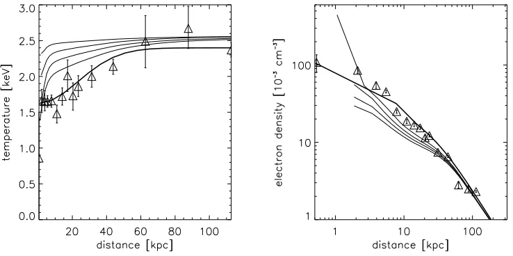
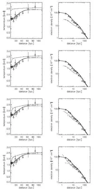
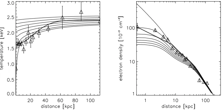
Figure 2.Temperature and density profiles evolving with time for simulation 0κ(see table 1). The thick lines for both temperature and density are the functions fitted to the data points (triangles) by Ghizzardi et al. (2004). The top line in the temperature plot shows the temperature profile after 3.17×₁₀8 _{yr and the bottom line at time of the end of the simulation. These times are given in table 1 for} each simulation. The intermediate lines represent the temperatures at intervals of 3.17×₁₀8 _{yr after the top temperature profile. The}

temporal sequence of the lines is reversed (bottom to top) in the density plot.

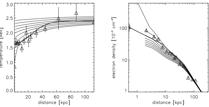
Figure 4.Temperature and density profiles evolving with time for simulation 0.1κ.

Figure 5. Temperature and density profiles evolving with time for simulation 1κ. Note that in this figure the temperature and density are plotted at intervals of 6.34×₁₀8_yrs.

cally. The fall in central temperature and rise in central den-sity that we observe are both the obvious signs of a strong cooling flow and eventually a cooling catastrophe in which large quantities of gas are being deposited into the central regions of the cluster.

It is evident from figures 2 to 5 that for increasing ther-mal conductivity the fit of the simulated density profiles to the observational data improves at larger radii. However, the profiles are not stable over sufficiently long timescales, e.g. the Hubble time. Thus, thermal conduction only delays the occurance of a cooling catastrophe and cannot simula-taneously reproduce temperature and density profiles that are consistent with observations.

4.2 Emissivity Profiles

From the simulated density and temperature data it is possi-ble to derive X-ray surface brightness maps for our radiative

cooling function. Previously we have compared the density and temperature distributions of our simulated clusters with those derived from observations of the X-ray surface bright-ness of the gas, since these are the fundmental variables used by FLASH. However, calculating the surface brightness for our simulations allows for a more direct comparison with the observational data. In practice the surface brightness along a given line of sight is dominated by emission from gas at the smallest radii from the cluster centre along that particular line of sight. Thus we calculate the emissivity of the gas (ǫ), i.e. the rate of energy loss per unit volume, and plot this as a function of radius. The bolometric emissivity is given by

ǫ=nenpΛrad(T, Z) [erg s−1cm−3] (13)

Figures 6 to 7 show the emissivity after 6.34_×108 _yrs

currently observed emissivity calculated from the work of Ghizzardi et al. (2004).

XMM-Newton observations revealed that the X-ray sur-face brightness was less centrally peaked than expected (e.g. Fabian et al. 2002). From figures 6 to 7 it is evident that our simulated clusters always develop a strong central peak in the surface brightness distribution, whether or not thermal conduction is taken into account. Such a peak is to be ex-pected given the density profiles in section 4.1, but is not present in the observational data. This again indicates that an extra heating mechanism in the central few kiloparsecs is required to prevent the excessive central cooling.

We note that the general fit at large radii to the obser-vational data seems to improve as the value of the thermal conductivity is increased. In addition, the emissivity pro-files show more excess emission out to larger radii for the simulations with a larger thermal conductivity. Thus, the emissivity plots re-iterate the previous observation from the density profiles that for higher thermal conductivities there is more mass in the central 20-50 kpc than for lower values of thermal conductivity. This is consistent with the mass flow rates which are larger at all radii for later times in the presence of high thermal conductivity than those for lower thermal conductivity (see section 4.5). Hence, in or-der to better match the observations by preventing a cooling catastrophe it appears that the presence of a larger thermal conductivity actually requires the input of more thermal en-ergy. In addition, this heat source would need to distribute its energy out to larger radii for the cases of larger thermal conductvity. The extra energy input required is roughly pro-portional to the extra volume which requires heating, and so an ICM with large thermal conductivity could require 100-1000 times more energy than for smaller thermal con-ductivities.

4.3 Effective Adiabatic Index

As an additional diagnostic for the behaviour of the clus-ter gas we calculate the effective adiabatic index defined by

γeff _≡ d lnP/d lnρ where P is the gas pressure, and ρ is the gas density. Following the method of Birnboim & Dekel (2003) we calculateγeff for a situation in which the volume of gas is constant, but is subjected to heating and cooling. The pressure in terms of the internal energy per unit mass,

e, is given by

P = (γ₋1)eρ[erg cm−3_{], (14)}

whereγis the true adiabatic index (e.g. 5/3 for a monatomic gas)

The rate of change of gas pressure with time is given by

˙

P= (γ₋1)( ˙eρ+eρ˙) [erg cm−3 _s−1_{]. (15)}

The rate of change of internal energy per unit mass for a constant volume of gas subjected to heating and cooling is given by

˙

e=h₋q [erg g−1_{], (16)}

where h and q are the heating and cooling functions per unit mass respectively.

By converting all the relevant quantities to be compat-ible with those we have defined previously and using the definition of the effective adiabatic index we findγeff to be given by

γeff = 1 + (γ₋1)

n2H−n2Λrad

˙

nkBT

, (17)

where H is the heating function (the heating analogue of the cooling function, Λrad), ˙n is the rate of change of number

density with time and the other symbols have their usual definitions.

In this derivation the nature of the heating and cool-ing mechanisms is not important, however, we choose to represent them in terms of quantities that we have already defined. From equation (17) we see that in the limit where either there is no heating or cooling or these competing ef-fects balance, the effective index is 1, which corresponds to an isothermal equation of state. Furthermore, we note that in the cases where no heating occurs,γeff is always less than one and for extreme cases will tend to zero as ˙n tends to

n/tcool(wheretcoolis the radiative cooling time). For a con-stant pressure cooling flowγeff will be equal to 1/3. In the cases where heating occurs this will have the effect of increas-ingγeff. Using this equation we predict for the simulations which include thermal conductivity at a significant fraction of the Spitzer value that the gas exhibits aγeffthat is greater than for lower values of thermal conductivity, at least in the cluster centre where radiative cooling is strongest.

In figure 8 we compare the effective adiabatic index ob-tained from the results of Ghizzardi et al. (2004) withγeff

for simulations 0κand 1κ. We note that in the absence of thermal conductivityγeff is roughly equal to 1 (isothermal) in our simulation only in the outer regions of the cluster, but falls steeply inside the central 10 kpc towards the cen-tral value given in table 2. The upturn at roughly 3 kpc is probably due to compressional heating towards the end of the simulated time. We also note that there is a minimum at roughly 25 kpc and a peak at roughly 15 kpc. For the full Spitzer value of thermal conductivity,γeff follows roughly a similar pattern to the above except that the variation is smoother. In addition, the central effective adiabatic index is higher due to the heating effect of thermal conductivity. In comparison, it is evident that for the functions fitted to the observational data by Ghizzardi et al. (2004)γeff is isother-mal throughout the cluster except for around 30 kpc where we observe a minimum similar to that noted in the simula-tion data. Of particular interest is the fact that there are 4 data points between the radii of 4-12 kpc with an effective adiabatic index of roughly 1 that are not consistent with either of the two simulations. By equation (17) this value of the observedγeff must be due to heating balancing cooling. From the simulations we can see that such a profile forγeff

is unattainable with thermal conductivity alone. Therefore, this is strong evidence that the Virgo cluster is being heated in the central regions by a mechanism other than thermal conduction.

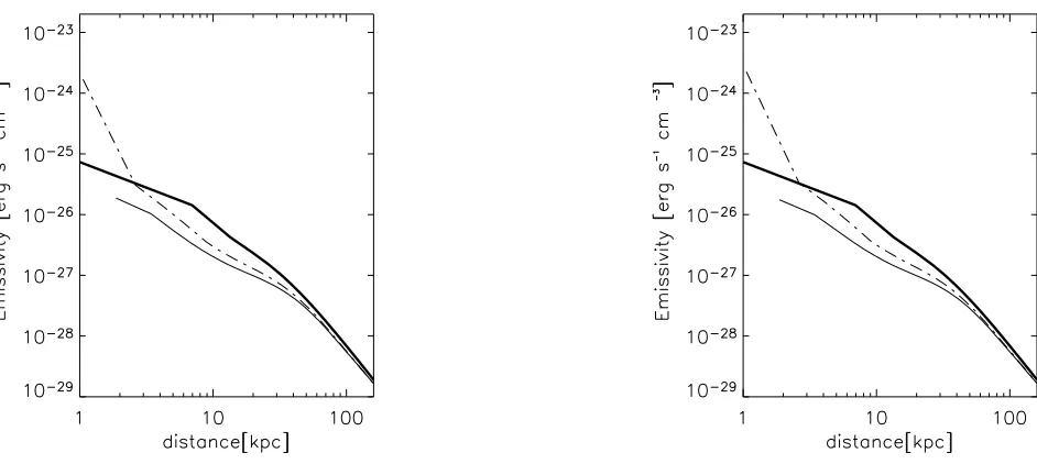
observa-Figure 6.Emissivity profiles for (from left to right) simulation 0κand 100κ. The thick line shows the observed emissivity given by Ghizzardi et al. (2004), the thin solid line shows the emissivity after 6.34×₁₀8 _{yrs; the thin dashed line shows the emssivity at the end}

point of each simulation as given by table 1.

Figure 7.Emissivity profiles for (from left to right) simulation 0.1κand 1κ. The definitions for each line are as in figure 6.

tional dataγeff appears to vary significantly throughout the cluster. Our results suggest that large values of the thermal conductvity tend to smooth out variations ofγeff. In addi-tion, since thermal conductivity acts to reduce the tempera-ture gradient, any heating source located near the centre of a cluster in which thermal conduction operates at near the Spitzer value is likely to result in a much flatter temperature profile than is currently observed. In the case where thermal conduction is heavily suppressed, it is possible that an ad-ditional heat source could maintain the temperature in the cluster centre at the observed level while allowing the region outside to continue to cool radiatively and thus produce the

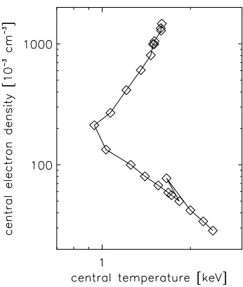
Figure 9.Central density against central temperature evolving as a function of time for simulation 0.01κ. The bottom right of the plot corresponds to the initial conditions and the system progresses upwards with passing time.

Figure 8.Comparison of the effective adiabatic index for simu-lation 1κ(triple dot dash), 0κ(dot dash) and the effective index from the fits to the observational data (solid line) and the data points. The triangles show the observational data that the fits are based on. At no point in time does the simulation data, within the central 15 kpc, approximate to the observational data. Therefore, for clarity, theγeff profiles for the simulation data are calculated

for times where the central temperature is near its lowest point. The vertical line near the left of the figure is the error bar from the data point closest to the cluster centre.

4.4 Central Temperature and density

It is also instructive to plot the central density against cen-tral temperature, at various points in time throughout each simulation. Figure 9 shows this for simulation 0.01κ. Each simulation shows the same three main characteristics: an

ini-tial power-law dependence between falling temperature and increasing density followed by a turning point near which the temperature begins to increase up to an asymptotic value while the density continues to increase. The results for each individual simulation are given in table 2 whereaandbare defined by a power-law relating temperature and density:

n=bTa_{. Given that the early evolutionary behaviour of the} central temperature and density is accurately described by a power-law it is also appropriate to describe this behaviour in terms of an effective adiabatic index, γeff which for the specified power-law is given by 1 + 1/a. The results given in table 2 show that the intial cooling phases are well de-scribed by power-laws and that a decreases for increasing values of thermal conductivity and b, which relates to the entropy, increases.γeff increases for larger thermal conduc-tivities because of the heating effect of thermal conduction in the cluster centre.

After the initial cooling in which the temperature falls with time, we observe without exception a period in which the central temperature begins to rise to an asymptotic value of roughly 1.6 keV which appears to be the same for each simulation. We have been unable to investigate the be-haviour past this asymptotic point due to the smallness of the timestep at the time when this behaviour was observed. The temperature rise is probably due to the cooling catastrophe which occurs after 109 _{yrs. The rapid inflow}

of material in the cluster centre results in some compres-sional heating. After a certain time the central tempera-ture has reached its maximum and begins to decrease again. Throughout this behaviour the density continues to increase while the temperature probably oscillates around the asymp-totic value to some degree.

find no evidence for a shock occuring near or after the turn-ing point. It appears that the power-law observed in these simulations and the other notable characteristics are unaf-fected by increasing the numerical resolution, see Appendix A.

4.5 Mass deposition rates

In this Section we calculate mass flow rates as a function of radius. Thus we can directly estimate the rate at which gas flows in to the cluster centre for different thermal conduc-tivities. In addition, we also calculate theoretical mass flow rates and compare them to the results from our simulations. The mass deposition rate is given by the mass flux through a spherical surface

dM

dt =

Z

ρv_.dA_{= 4πr}2_{ρvr [g s}−1_{], (18)}

where vr is the projection of the velocity vector on to the radial vector.

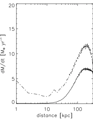
Figures 10 to 11 show the mass deposition rates as a function of radius for two different times. These figures show the local mass flow rates and not the integrated mass flow rate, M(<r). The first line (solid) is the mass deposition rate profile after 6.34_×108 yrs, the second line (dashed) is the profile for the final point in the simulation given in table 1. For the mass flow rate profiles after 6.34_×108 _{yrs the}

flow rate tends to zero in the cluster centre in all simulations. There is also a point near 150 kpc at which the flow rate reaches a maximum. From here on we refer to this point as the break-radius (Edge et al. 1992; Allen et al. 2001). The increase outside the break-radius (at roughly 200 kpc) is probably not realistic, but is due to edge effects in which the initial velocities are large, but dissipate over the duration of the simulation.

For the later profiles, when the cooling flow is well es-tablished, the central mass deposition rate increases up to several solar masses per year in all cases. We also note that the break-radius has moved further away from the cluster centre. The peak mass flow, at the break radius, is smaller for larger values of thermal conductivity. This is possibly a consequence of the action of shear viscosity which slows the inflow of the gas. In addition, the width of the mass flow rate peak increases with increasing thermal conductiv-ity and viscosconductiv-ity, indicating that in such cases there is more mass flowing towards the centre and that the inflow velocity falls off less quickly with radius. Thus it is possible that the central galaxies in clusters, which are thermally conducting, may be more massive, by a factor of a few, than those in cluster in which thermal conduction does not occur.

The calculated mass deposition rates are important for comparison with observational results. Edge (2001) finds the mass of molcular gas around M87 to be less than 1.3_×108_M

⊙. If the Virgo cluster has been cooling for roughly 10 Gyr then the average mass deposition rate over this pe-riod cannot be greater than 0.013 M⊙yr−1. We find that for a thermal conductivity at the Spitzer value the mass deposi-tion rate in the centre of the cluster is negligible for the first

∼109 years, but rises to several M⊙yr−1thereafter. In ad-dition, the rate of mass deposition will continue to increase after this time as the cooling catastrophe accelerates. For

the cases with suppressed thermal conductivity the central mass deposition rate is significant from earlier times mean-ing that more gas is deposited in the cluster centre for these simulations. Therefore, although the central mass flow rates of a few M⊙yr−1 appear at first rather modest, it is worth noting that the mass flow rates in the centre will quickly exceed the observations‘ upper limit.

It is possible to compare the calculated mass flow rates from our simulations with analytical predictions. In order to do this we require both the density and velocity profiles. However, it is not possible to solve the full hydrodynamic equations analytically for the velocity profile as a function of time due to the complexity of the problem. Instead we use both observational and simulation data to constrain the functional form of the velocity profile at any given time.

Figures 10 and 11 show that there is clearly a break radius in the mass flow rate profiles which agrees with the observations of Edge et al. (1992) and Allen et al. (2001). However, unlike these authors we plot the mass flow rate at each radius and not the cumulative mass flow rate. Since the radiative cooling rate is greatest near the cluster centre, gas in the central regions will lose its pressure support. This means that not only would we expect the gas infall velocity to tend asymptotically to zero for large radii, but that the scale height of the velocity profile will increase as a function of time as the less dense gas at larger radii has time to cool. The radiative cooling time as a function of radius is given by equation (7). We assume the cluster gas to be isothermal and the density to follow a generalisedβ-profile. Rearranging for the radius, we arrive at the cooling radius as a function of time

rcool r0 =

2tΛrad0n0

3kBT0.5

32β

−1

12

, (19)

wherer0 is the scale height of the density distribution. For the Virgo cluster the value of β is roughly 0.47 for radii greater than roughly 30 kpc.

Equation (19) implies that after times of order 0.3 Gyrs the velocity scale height grows proportional tot1/(3β).

Further constraints on the velocity profile can be deter-mined using equation (18) and what we already know about the gas density of the Virgo cluster. The electron number density given by equation (10) implies that at large radii the density scales as r1.4_{. Substituting this into equation}

(18) implies that in order for there to be a break radius the infall velocity of the gas must fall off more quickly than approximatelyr−0.6_{. Furthermore, by the observation that}

the mass flow rate tends asymptotically to zero in the clus-ter centre (before the cooling catastrophe occurs) it follows that, at least, in the central region the velocity cannot fall off faster thanr−2_{. However, it should be noted that after the}

occurance of the cooling catastrophe the central mass flow rate becomes finite. This suggests that the velocity profile steepens at least in the central few kiloparsecs and may be an indication that the gas is in free-fall after the onset of the cooling catastrophe. Thus, for the Virgo cluster, if the infall velocity follows a power-law (v∼r−α_{) thenαmay be} con-strained to lie between 0.6 and 2. In general, for any cluster in which the gas density may be described by aβ-profile the constraints onαare (2 - 3β)6α62.

veloc-Table 2.Summary of the parameters describing the behaviour of the central temperature and density for each simulation. The temperatures are given in keV and densities in units of 103cm−3

κ/κS a b γeff turning point(T,n) asymptote(T)

0 -1.60±_{0.025 -30.7}±_{0.41 0.375}±_0.006 ≃_0.84,≃₁₅₁ ≃_1.6 0.01 -1.67±_{0.016 -29.7}±_{0.27 0.40}±_0.004 ≃_0.89,≃₁₄₉ ≃_1.6 0.1 -1.96±_{0.119 -24.5}±_{1.95 0.49}±_0.029 ≃_0.94,≃₂₁₂ ≃_1.6 1 -2.32±_{0.070 -18.4}±_{1.17 0.57}±_0.017 ≃_0.82,≃₂₇₀ ≃_1.6

Figure 10.Mass deposition profiles for (from left to right) simulations 0κand 0.01κ. In all plots the solid line shows the mass flow rate at 6.34×₁₀8 _{yrs; the dashed line refers to the end point in the simulation. The times of the end points are given in table 1.}

ity profile we adopt a velocity profile as v_∼exp(₋r2/rs2) which satifies the condition above, where rs is the scale height of the velocity profile which is equivalent to the cool-ing radius described in equation (19).

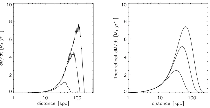
In order to understand the dependence of the mass flow rate on velocity we use the density profile that we calculated for the initial conditions of these simulations and the veloc-ity profile described above and vary only the velocveloc-ity scale height with time. The peak mass flow rate is determined by the velocity in the cluster centre, which by comparison with the simulation we chose to be of order 105_{cm s}−1_{. The}

sity profile can be assumed to remain fixed since the den-sity should not change significantly until a cooling catas-trophe occurs. However, a gradual increase in the central density will inevitably occur due to the inflow of gas to-wards the cluster centre. The results of this basic analysis are compared to the simulation data in figure 12. It is ob-vious that despite the simplistic nature of the analysis its predictions match the simulation results reasonably well. In addition, the analysis should hold for clusters in general and not just the Virgo cluster. Thus our inflow velocity profile,

v_∼exp(₋r2_/rs2_{), can be taken as a generic approximation}

for the gas velocity in radiatively cooling clusters.

5 SUMMARY

Our results suggest that thermal conduction is unable to prevent the occurance of a cooling catastrophe and can only increase the cooling time in the cluster centre by a factor of a few. Tests using different coordinate systems and spatial resolutions show that the developement of a cooling catas-trophe is inevitable. We do not consider this to be a con-sequence of our chosen initial conditions since we allow the cluster to evolve self-consistently, taking into account all rel-evant physics of which we are aware, using standard intial conditions used in cluster formation theory.

The temperature and density profiles from our simu-lated clusters fail to simultaneously converge to the observa-tional constraints. The mass flow rates we calculate also sug-gest that significantly more mass is deposited in the cluster centre than is observed. Somewhat contrary to expectations we also find that the mass flow rates are also greatest for the simulations in which thermal conductivion is most im-portant. The extra central concentration of mass this causes results in emissivities with broader peaks than for lower ther-mal conductivities. A consequence of this is that for these cases more energy has to be injected, for example, by a cen-tral AGN than for more weakly conducting cases to avert a cooling catastrophe.

These results are in agreement with Voigt et al. (2002) who found that in their sample thermal conduction could only balance radiative losses in the outer regions of clus-ter cores. There is a slight contradiction with the find-ings of Zakamska & Narayan (2003) who found that the temperature and density profiles of several galaxy clusters were consistent with a steady state maintained by phys-ically meaningful values of thermal conduction. However, since Zakamska & Narayan (2003) do not take into account the effect of line cooling, which is more significant at the lower temperatures near cluster centres, and only look for the temperature and density profiles which will ensure a

steady state, it is unclear whether this study and ours are comparable. Furthermore, neither of Voigt et al. (2002) nor Zakamska & Narayan (2003) have made predictions about the Virgo cluster. It would therefore be of interest to un-dertake a similar study, to this, for a cluster for which Zakamska & Narayan (2003) suggest thermal conduction could maintain a steady state.

The simulated and observed effective adiabatic index indicates that there is a heat source at the centre of the Virgo cluster. In addition, given this and the temperature and density profiles we suggest that thermal conductivity is suppressed to at most 1/100 to 1/10 of the full Spitzer value. However, even if thermal conductivity and viscosity are suppressed by a factor of 100, the thermal conduction and viscous dissipation of sound waves generated in the ICM could be significant.

For the overall energy budget we suggest that thermal conduction is unlikely to be able to suppress the cooling in the majority of clusters. The reason for this is simple: the physics underlying thermal conduction and radiative cooling is too different for the two processes to balance each other. The fact that these energy terms cannot balance means that the temperature and density profiles are likely to be unstable on cosmologically relevant timescales. Thermal conductivity cannot be responsible for the universal temperature profiles of clusters as observed by Allen et al. (2001).

6 ACKNOWLEDGEMENTS

ECDP acknowledges support from the Southampton Re-gional eScience centre in the form of a studentship. GP and CRK thank PPARC for rolling grant support. The soft-ware used for this work in part developed by the DOE-supported ASCI/Alliance Center for Astrophysical Ther-monuclear Flashes at the University of Chicago. We would like to thank the anonymous referee for helpful comments.

REFERENCES

Allen S. W., Fabian A. C., Johnstone R. M., Arnaud K. A., Nulsen P. E. J., 2001, MNRAS, 322, 589

Allen S. W., Schmidt R. W., Fabian A. C., 2001, MNRAS, 328, L37

Birnboim Y., Dekel A., 2003, MNRAS, 345, 349 Br¨uggen M., 2003, ApJ, 593, 700

Br¨uggen M., Kaiser C. R., 2002, Nat., 418, 301 Carilli C. L., Taylor G. B., 2002, ARA&A, 40, 319 Cho J., Lazarian A., Honein A., Knaepen B., Kassinos S.,

Moin P., 2003, ApJ, 589, L77

Choudhuri A., 1998, The Physics of Fluids and Plasmas, an introduction for astrophyisicists. Cambridge University Press

Churazov E., Br¨uggen M., Kaiser C. R., B¨ohringer H., For-man W., 2001, ApJ, 554, 261

Cowie L. L., McKee C. F., 1977, ApJ, 211, 135

Dalla Vecchia C., Bower R. G., Theuns T., Balogh M. L., Mazzotta P., Frenk C. S., 2004, MNRAS, 355, 995 Dolag K., Jubelgas M., Springel V., Borgani S., Rasia E.,

2004, ApJ, 606, L97

Figure 12.Comparison of the mass flow rates for increasing time for simulation 0.01κdata (left) and from simple theoretical predictions at the same times.

Edge A. C., Stewart G. C., 1991, MNRAS, 252, 414 Edge A. C., Stewart G. C., Fabian A. C., 1992, MNRAS,

258, 177

Ettori S., Fabian A. C., 2000, MNRAS, 317, L57 Evrard A. E., 1990, ApJ, 363, 349

Fabian A. C., 1994, ARA&A, 32, 277

Fabian A. C., Allen S. W., Crawford C. S., Johnstone R. M., Morris R. G., Sanders J. S., Schmidt R. W., 2002, MNRAS, 332, L50

Fryxell B., Olson K., Ricker P., Timmes F. X., Zingale M., Lamb D. Q., MacNeice P., Rosner R., Truran J. W., Tufo H., 2000, ApJ Supp., 131, 273

Ghizzardi S., Molendi S., Pizzolato F., De Grandi S., 2004, ApJ, 609, 638

Kaiser C. R., Pavlovski G., Pope E. C. D., Fangohr H., 2005, ArXiv Astrophysics e-prints

Loeb A., 2002, New Astronomy, 7, 279 Malyshkin L., Kulsrud R., 2001, ApJ, 549, 402

Markevitch M., Mazzotta P., Vikhlinin A., Burke D., Butt Y., David L., Donnelly H., Forman W. R., Harris D., Kim D.-W., Virani S., Vrtilek J., 2003, ApJ, 586, L19

Narayan R., Medvedev M. V., 2001, ApJ, 562, L129 Navarro J. F., Frenk C. S., White S. D. M., 1995, MNRAS,

275, 56

Navarro J. F., Frenk C. S., White S. D. M., 1997, ApJ, 490, 493

Nipoti C., Binney J., 2004, MNRAS, 349, 1509 Ruszkowski M., Begelman M. C., 2002, ApJ, 581, 223 Rybicki G. B., Lightman A. P., 1979, Radiative Processes

in Astrophysics. Wiley-Interscience

Sarazin C. L., 1986, X-ray Emission from Clusters of Galax-ies. Reviews of Modern Physics

Spitzer L., 1962, Physics of Fully Ionized Gases. Wiley-Interscience, New York

Sutherland R., Dopita M., 1993, ApJ Supp., 88, 253 Tabor G., Binney J., 1993, MNRAS, 263, 323 Tribble P. C., 1989, MNRAS, 238, 1247

Vikhlinin A., Markevitch M., Forman W., Jones C., 2001, ApJ, 555, L87

Voigt L. M., Fabian A. C., 2004, MNRAS, 347, 1130 Voigt L. M., Schmidt R. W., Fabian A. C., Allen S. W.,

Johnstone R. M., 2002, MNRAS, 335, L7 Woodward P., Colella P., 1984, JCP, 54, 174 Zakamska N. L., Narayan R., 2003, ApJ, 582, 162

APPENDIX A: NUMERICAL RESOLUTION CONVERGENCE

The numerical convergence of the simulations was tested by running simulation 0.01κwith varied spatial resolution. We compare the evolution of temperature and density profiles for otherwise identical simulations in which the minimum refinement, maximum refinement and region of increased initial resolution in the central region are all increased by one level of refinement. For the size of the computational box we employ for these simulations, a refinement level of 9 corresponds to a resolution of 0.31 kpc; a refinement level of 10 corresponds to 0.15 kpc. The initial enhanced resolution of the central region (refinement of 6) corresponds to 2.53 kpc in the central_∼16 kpc. We also investigate the effect of increasing this resolution by one level of refinement to a res-olution of 1.26 kpc. The resres-olution in the outer regions of the cluster is determined by the minimum refinement level. This is initially set to 3 (corresponding to roughly 20 kpc), but is also tested at level 4 (roughly 10 kpc). The refinement pa-rameters corresponding to each simulation are summarised in table A1.

Table A1.Summary of the refinement parameters of the numerical resolution tests.

Test Central Refinement Maximum refinement Minimum refinement

1 7 9 3

2 6 9 3

3 7 10 3

4 8 9 3

5 7 9 4

changed and in good agreement across the range of different resolutions. This series of tests demonstrates that for a cen-tral refinement of level 7, a maximum refinement of level 9 and a minimum refinement of level 3 the results are in close agreement with those achieved with higher resolutions.

APPENDIX B: HYDRODYNAMIC DIFFERENCES BETWEEN 3-D AND 1-D COORDINATE SYSTEMS GEOMETRIES

In this section we outline the differences between a purely spherically symmetric geometry and a full 3-d geometry, for our problem, with the aid of the hydrodynamic equations and trial simulations of the Virgo cluster. For these pur-poses we have re-done two of the simulations from the main paper with i) zero thermal conductivity and viscosity and ii) full Spitzer thermal conductivity and viscosity, in 1-d spherical coordinates, both at the same spatial resolution as our 3-d runs and higher spatial resolutions. The minimum level of refinement for the 1-d simulation performed at the same spatial resolution as the 3-d runs was 7 correspond-ing to roughly 1.27 kpc. For the higher spatial resolution 1-d test the minimum refinement was level 9, correspond-ing to a spatial scale of nearly 0.32 kpc. In both cases the maximum level of the refinement was 12 corresponding to approximately 0.04 kpc.

The results of these 1-d spherically symmetric simula-tions explicitly show that a cooling catastrophe always oc-curs in 1-d as well as 3-d. Furthermore, the cooling catastro-phe takes less time to evolve in the 1-d scatastro-pherically symmetric case than the 3-d case and increasing spatial resolution has almost no effect. For the simulation with zero thermal con-ductivity the cooling catastrophe occurs after approximately 1_×109_{yrs-roughly 3}

×108 _{yrs before the occurance in 3-d.}

For the simulation with full Spitzer thermal conductivity the cooling catastrophe occurs after roughly 4.2_×109_{yrs which}

is approximately 0.5_×109_{yrs less than in the 3-d case (see}

figures B1 and B2).

Figure B3 gives an indication of the non-radial flow in the central regions of our simulated clusters, in the absence of thermal conduction and viscosity. If the differences for simulations using different geometries are real physical ef-fects, rather than numerical errors, then we should also ex-pect to see differences in the equations of hydrodynamics for the 1-d and 3-d cases. Since viscosity enters into the mo-mentum equation it is an appropriate choice to investigate any differences which may arise due to dimensional effects.

The equation for the viscous force per unit volume is given by (e.g. Sarazin 1986)

F_vis=η

∇2v₊1

3∇∇.v

, (B1)

whereηis the bulk viscosity andvis fluid velocity. Using the standard vector identity we can substitute for the divergence term

∇2v₌∇(∇.v₎₋∇_×(∇_×v_{) (B2)}

so that equation (B1) becomes

F_vis=η

4 3∇

2_v+1

3∇×(∇×v)

. (B3)

Even without the evidence from simulations, from equa-tion (B3) alone it is evident that viscous processes are differ-ent in 3-d and 1-d cases due to shear effects. In 3-dimensions the term involving the vector products constitutes a mech-anism for the dissipation of momentum, whereas in 1-d all vector products are zero, by definition, and so this mecha-nism is suppressed.

It seems that equation (B3) is able to account for some of the differences between the 1-d and 3-d simulations in which full Spitzer thermal conductivity and viscosity were present. However, there was also a significant difference in the time at which the cooling catastrophe occured in the simulations in which diffusion processes were not present. Studying the complete momentum equation allows us to in-vestigate these differences.

∂v

∂t + v.∇

v=F ₋1

ρ∇P+ν

₄

3∇

2_v+1

3∇×(∇×v)

,

(B4) whereF is the force per unit mass, P is the fluid pressure andνis the kinematic viscosity.

Using a second standard vector calculus identity for the second term on the left hand side of equation (B4) we find

v_.∇ v₌1

2∇(v.v)−v×(∇×v), (B5) and substituting into equation (B4), the total momentum equation is

∂v

∂t+

1

2∇(v.v)−v×(∇×v) =F− 1

ρ∇P+ν

₄

3∇

2_v+1

3∇×(∇×v)

.

(B6) Since vector products are zero in 1-dimension, equation (B6) reduces to

∂v ∂t +

1 2

∂(v2₎ ∂r =F−

1

ρ ∂P

∂r +ν

4 3 1 r2 ∂ ∂r

r2∂v ∂r

Figure B1.Temperature and density profiles evolving with time for simulation 0κfor a 1-d spherically symmetric geometry. The profiles are plotted for the same times as the equivalent temperature and density profiles in section 4.1, with the same spatial resolution, except for the final profile which is plotted at 1×₁₀9_yrs.

Figure B2.Temperature and density profiles evolving with time for simulation 1κfor a 1-d spherically symmetric geometry. The profiles are plotted for the same times as the equivalent temperature and density profiles in section 4.1, with the same spatial resolution, except for the final profile which is plotted at 4.2×₁₀9_yrs.

in 1-d spherically symmetric coordinates.

From equation (B7) it is clear that there is an additional dissipation term in the 3-d case which is not present in 1-d, even in the absence of viscosity. Thus, in agreement with our simulations, it is reasonable to expect the behaviour of a fluid to be different in 1-d compared to 3-d, even in the absence of viscosity.

We note that the overall properties of the simulations, e.g. the temperature and density profiles, remain roughly the same in 1-d spherically symmetric and 3-d coordinates. Therefore, for simulations such as these it seems possible to gain a reasonable estimate of the main properties and timescales for the given circumstances at a lower compu-tational expense than for 3-d simulations. However, in or-der to gain a more complete unor-derstanding of the physical