Discrete Predictive Optimal ILC Implemented on a Non-minimum
Phase Experimental Test-bed
Chris Freeman, Paul Lewin and Eric Rogers
Abstract— Predictive Optimal ILC has been implemented on a non-minimum phase experimental test facility. Predictive Optimal ILC has first been derived for discrete-time systems, having previously only been formulated for the continuous case. Practical implementation issues have been considered and methods have been proposed to limit the necessary memory and calculation time required. The plant has been described and experimental results then presented for two cases of predictive horizon. The effect of variation of parameters used in the cost function has been described. The convergence rate observed in practice has been compared against a theoretical bound.
I. INTRODUCTION
Iterative learning Control (ILC) can be applied to systems which repetitively perform the same task with a view to sequentially improving accuracy. The task in question is regarded as the tracking of a given reference signal r(t) or output trajectory for an operation on a specified time interval. The object of ILC is to use the repetitive nature of the process to progressively improve the accuracy with which the operation is achieved by updating the control input iteratively from trial to trial. A literature survey of ILC can be found in [1] and there exist textbooks on the subject [2], [3].
Norm Optimal ILC and Predictive Optimal ILC (which includes Norm Optimal ILC as a subset) have been im-plemented on a non-minimum phase experimental test-bed. Non-minimum phase systems have proved a significant challenge in the field of ILC and the experimental test-bed was designed specifically to include this characteristic. The Norm Optimal algorithm has previously been derived both in continuous time [4] and discrete time [5], [6]. The Predictive Optimal ILC law has been derived in continuous time only [7]. The absence of a discrete formulation of Pre-dictive Optimal ILC necessitates its derivation here before it can be implemented on an experimental non-minimum phase spring-mass-damper system. The formulation of Pre-dictive Optimal ILC for discrete systems closely follows the continuous case, the signal norms used, however, are the same as those used in the discrete derivation of Norm Optimal ILC [6].
II. ALGORITHM DERIVATION
The Predictive Optimal ILC problem is set up as in [6], using k to denote the trial index, and t the elapsed time during the trial. The trial is of length M samples and the C. Freeman, P. Lewin and E. Rogers are with the School of Electronics and Computer Science, University of Southampton, University Road, Southampton SO17 1BJ, United Kingdom, email: [email protected]
reference is denoted by r(t). The ILC process is said to be convergent if and only if{uk(t)}k≥0, when applied to the plant, produces an output sequence{yk(t)}k≥0 with the property that the following limits exist:
limk→∞yk(t) =r(t) limk→∞uk(t) =u∞(t)
∀t∈[0, M] (1)
In this paper the following sampled-time system is consid-ered
x(t+ 1) =Ax(t) +Bu(t) x(0) =x0 0≤t≤M
y(t) =Cx(t) x∈Rn, u∈Rm, y∈Rp (2) The state-space matrices A, B, C are assumed to be time-invariant for simplicity. Because only finite time intervals are considered in ILC, the output can be written in vector form by defining the supervectors
y=
⎡ ⎢ ⎢ ⎢ ⎣
y(1) y(2)
.. .
y(M)
⎤ ⎥ ⎥ ⎥
⎦ u=
⎡ ⎢ ⎢ ⎢ ⎣
u(0) u(1)
.. .
u(M−1)
⎤ ⎥ ⎥ ⎥
⎦ (3)
An equivalent representation of (2) becomes
y=y0+Gu (4)
with the matrixG∈R(pM)×(mM) defined as
G=
⎡ ⎢ ⎢ ⎢ ⎣
CB 0 . . . 0
CAB CB . . . 0
..
. ... . .. ...
CAM−1B CAM−2B . . . CB
⎤ ⎥ ⎥ ⎥
⎦ (5)
with the vector of initial condition response y0 =
[(CA)T (CA2)T . . . (CAM)T]Tx
0. The matrix G is invertible in the SISO case if and only if CB = 0, and if it has a delay, can be regularised (see [6]). Consider a tracking problem with reference trajectory r(t), given for
1≤t≤M (a relative degree of 1 is assumed for simplicity of representation). The tracking error is defined as
e=r−y=r−Gu−y0= (r−y0)−Gu (6) whereeandrare supervectors. Without loss of generality, it is possible to replacerbyr−y0in the analysis and thence assume thaty0= 0or, equivalently,x0= 0. On completion of thekthtrial, the Predictive Optimal algorithm calculates the control input on the (k+ 1)th trial as the solution of the minimum norm optimisation problem:
uk+1= arg min
uk+1{Jk+1:ek+1=r−yk+1, yk+1=Guk+1}
(7)
2005 American Control Conference
The discrete form of the cost appearing in [7] is written as
Jk+1,N = N
i=1
λi−1(e
k+i2Y+uk+i−uk+i−12U) (8)
and, with N = 1, this reduces to the cost used in [6]. The parameter λ > 0 is used to determine the importance of future errors. The norms · are appropriate norms for the input and outputUandYspaces respectively. These spaces arel2 spaces ofmandpvectors on[0, M−1]and[1, M]. Written out as sums the index becomes
Jk+1,N = N
i=1
λi−1 M
t=1
[r(t)−yk+i(t)]TQ(t)[r(t)−yk+i(t)]
+
M−1
t=0
[uk+i(t)−uk+i−1(t)]TR(t)[uk+i(t)−uk+i−1(t)]
(9) The weighting matricesQ(t)andR(t)must be symmetric and positive definite for all t. The cost function (8) is equivalent to (9) if the norms used are induced from the following inner products
y1, y2Y = yT1Qy2= M
t=1
y1(t)TQ(t)y2(t) (10)
u1, u2U = uT1Ru2= M−1
t=0
u1(t)TR(t)u2(t) (11)
Following the reasoning of the continuous case [7], it is postulated thatJk+1,N is a quadratic form inek, that is
Jk+1,N(uk+1) =ek, QNekY (12)
where QN ∈ R(pM)×(pM) is a symmetric matrix. We can then write
Jk+1,N =ek+1Y2+uk+1−uk2U
+λ
N−1
j=1
λj−1(e
k+1+j2Y+uk+1+j−uk+j2U)
=ek+12Y+uk+1−uk2U+λJk+2,N−1 (13) The controller on the(k+ 1)thtrial is obtained with vector differential calculus from the required stationary condition,
1 2
∂Jk+1,N
∂uk+1 =−G TQe
k+1+R(uk+1−uk)+λ2∂J∂uk+2,N−1 k+1
= 0 (14) The postulate (12) allows the substitution Jk+2,N−1 =
ek+1, QN−1ek+1Y so that
∂Jk+2,N−1
∂uk+1 =−2G TQQ
N−1ek+1 (15) Inserting this into (14) and rearranging produces
uk+1 = uk+R−1GTQek+1+λR−1GTQQN−1ek+1
= uk+G∗ek+1+λG∗QN−1ek+1 (16)
The substitution G∗ = R−1GTQ can be made since
R−1GTQis equivalent to the adjoint operator with respect to the weighted inner product equations (10,7) [8]. Equation (16) is identical to the continuous time case and, setting
N = 1, equates to the discrete Norm Optimal solution, since
Q0= 0. Manipulation of (16) yields the error evolution
ek+1 =LNek, LN = [I+GG∗(I+λQN−1)]−1 (17) whereLN ∈R(pM)×(pM). To determineQN, (16) is used to write
uk+1−ukU=
(R−1GTQ(I+λQ
N−1)ek+1)TR(R−1GTQ(I+λQN−1)ek+1) = (GT(I+λQN−1)ek+1)TQ(R−1GTQ(I+λQN−1)ek+1)
=ek+1,(I+λQN−1)GG∗(I+λQN−1)ek+1Y
(18) so that (13) becomes
Jk+1,N =ek+1, ek+1Y+λek+1, QN−1ek+1Y +ek+1,(I+λQN−1)GG∗(I+λQN−1)ek+1Y =ek+1,(I+λQN−1)[I+GG∗(I+λQN−1)]ek+1Y =ek, LN(I+λQN−1)ekY
(19) Comparison with (12) yields the following recursive equa-tion forQN:
QN = LN(I+λQN−1)
= [I+GG∗(I+λQ
N−1)]−1(I+λQN−1) (20) It is then possible to expressLN as a recursive relation by eliminatingQN
LN(H, λ) = [(1 +λ)I+H−λLN−1]−1, N= 1,2, . . . (21) where L0 = I, and H := GG∗ has been used for conciseness. LN(H, λ) is a symmetric matrix and, if H is positive and bounded in norm, is positive according to the bound
LN(H, λ)≥(I+λ+H)−1>0, ∀0< λ <∞, N = 1,2, . . . (22)
The upper bound of LN (the norm of LN) is important to ILC convergence since the norm of the error at the kth trial can be bounded byek ≤ LNke0. Therefore it is sufficient for convergence thatLN is less than one. If the plant is bounded below such that
e, HeY≥σ2e2Y ∀ e∈Y (23)
thenLN ≤lN(σ2, λ)I with
lN(σ2, λ) =
1
1 +λ+σ2−λlN−1(σ2, λ), l0= 1 (24) and the error sequence is bounded by ek+1 ≤
lN(σ2, λ)ek. If σ > 0 then LN < 1 ∀N ≥ 1 then geometric convergence is assured. In the case of N = 1 thenL1= [I+H]−1andl1=1+σ12 which agrees with the
rate of convergence seen in [6]. In the case ofN = 2then
L2 = [(1 +λ) +H −λ(I+H)−1)]−1 and we can write
l2 = 1+λ+σ2−1λ( 1
1+σ2) which will later be compared with
[6], σ can be changed by the design rates QandR since the definition of σcan be written as
eTGTQGe≥σ2eTRe ∀e∈Y (25)
III. CAUSAL ALGORITHM FORMULATION In this section the cost function (9) is transformed until it is in the form of
Jk+1,N =ek+12Y+uk+1−uk2U (26)
which is the cost function used in the discrete Norm Optimal ILC derivation [6]. The corresponding causal solution can then be applied to form the necessary update. In order to do this (9) is written out in full as
Jk+1,N = M t=1 ⎡ ⎢ ⎢ ⎣ ek+1 ek+2 . . .
ek+N ⎤ ⎥ ⎥ ⎦ T⎡ ⎢ ⎢ ⎣
Q 0 . . . 0 0 λQ . . . 0
. . . . . . .. . . . .
0 0 . . . λN−1Q ⎤ ⎥ ⎥ ⎦ ⎡ ⎢ ⎢ ⎣ ek+1 ek+2 . . .
ek+N ⎤ ⎥ ⎥ ⎦
+
M−1
t=0
⎡ ⎢ ⎢ ⎣
uk+1−uk uk+2−uk+1
. . .
uk+N−uk+N−1
⎤ ⎥ ⎥ ⎦ T⎡ ⎢ ⎢ ⎣
R 0 . . . 0 0λR . . . 0
. . . . . . .. . . . .
0 0 . . . λN−1R ⎤ ⎥ ⎥ ⎦ ⎡ ⎢ ⎢ ⎣
uk+1−uk uk+2−uk+1
. . .
uk+N−uk+N−1
⎤ ⎥ ⎥ ⎦
(27) Using the substitution
⎡ ⎢ ⎢ ⎢ ⎢ ⎣
uk+1−uk
uk+2−uk+1
uk+3−uk+2 .. .
uk+N−uk+N−1
⎤ ⎥ ⎥ ⎥ ⎥ ⎦ T = ⎡ ⎢ ⎢ ⎢ ⎢ ⎣
1 0 0. . . 0
−1 1 0. . . 0
0 −1 1. . . 0
..
. ... ... . .. ...
0 0 0. . . 1
⎤ ⎥ ⎥ ⎥ ⎥ ⎦ ⎡ ⎢ ⎢ ⎢ ⎢ ⎣
uk+1−uk
uk+2−uk
uk+3−uk .. .
uk+N−uk ⎤ ⎥ ⎥ ⎥ ⎥ ⎦ (28) the difference-in-input vector of (27) can be rewritten. The implementation uses a number of parallel plants, only the first of which is the actual plant which produces uk+1. The other ‘virtual’ plants are simulated, their only purpose being to contribute to the calculation of uk+1. The errors are written in vector form as
⎡ ⎢ ⎢ ⎣
ek+1
ek+2 .. .
ek+N ⎤ ⎥ ⎥ ⎦= ⎡ ⎢ ⎢ ⎣ r r .. . r ⎤ ⎥ ⎥ ⎦− ⎡ ⎢ ⎢ ⎣
G 0 . . . 0 0 G . . . 0
..
. ... . .. ...
0 0 . . . G
⎤ ⎥ ⎥ ⎦ ⎡ ⎢ ⎢ ⎣
uk+1
uk+2 .. .
uk+N ⎤ ⎥ ⎥
⎦ (29)
According to the block diagonal plant matrix from (29) the extended plant matrices are defined
AN =diag{A, A, . . . A}, BN =diag{B, B, . . . B}
CN =diag{C, C, . . . C}
(30)
and also the following extended weight matrices
QN =diag{Q, λQ, . . . λN−1Q},
RN =
⎡ ⎢ ⎢ ⎢ ⎢ ⎣
(1 +λ)R −λR 0 . . . 0
−λR (λ+λ2)R −λ2R . . . 0 0 −λ2R (λ2+λ3)R . . . 0
..
. ... ... . .. ...
0 0 0 . . . λN−1R
⎤ ⎥ ⎥ ⎥ ⎥ ⎦ (31) The optimisation problem is now in the form of the causal LQR prblem proposed in [6] which has the following solution
⎡ ⎢ ⎢ ⎣
uk+1
uk+2 .. . uk+N ⎤ ⎥ ⎥ ⎦= ⎡ ⎢ ⎢ ⎣ uk uk .. . uk ⎤ ⎥ ⎥
⎦−{BNTK(t)BN+RN(t)}−1BTNK(t)
×AN
⎛ ⎜ ⎜ ⎝ ⎡ ⎢ ⎢ ⎣
xk+1
xk+2 .. . xk+N ⎤ ⎥ ⎥ ⎦− ⎡ ⎢ ⎢ ⎣ xk xk .. . xk ⎤ ⎥ ⎥ ⎦ ⎞ ⎟ ⎟ ⎠ ⎤ ⎥ ⎥
⎦+RN−1(t)BNTξk+1,N(t)
(32) where the state feedback gain matrix K(t)is the solution of the discrete matrix Riccati equation on the interval t∈
[0, M−1]
K(t) =AT
NK(t+ 1)AN+CTNQN(t+ 1)CN−[ATNK(t+ 1)
×BN{BNTK(t+ 1)BN+RN(t+ 1)}−1BNTK(t+ 1)AN]
(33) with the terminal condition K(M) = 0. The feedforward termξk+1,N(t)is generated by
ξk+1,N(t) ={I+K(t)BNR−N1(t)BTN}−1
×{AT
Nξk+1,N(t+ 1) +CNTQN(t+ 1)
⎡ ⎢ ⎢ ⎣
ek(t+ 1)
ek(t+ 1) .. .
ek(t+ 1)
⎤ ⎥ ⎥
⎦}
(34) with the terminal conditionξ(M) = 0. The algorithm uses
N−1 models of the plant in parallel with the actual plant for the computation of the optimal input for the N-step predictive algorithm. Only knowledge of the state xk+1(t) of the actual plant is a potential problem as the others are directly available from the simulated plants. If it is not available an observer can be constructed to estimate it.
IV. NON-MINUMUM PHASE PLANT
2
2
J
B
K
J
oi
g
G
r
r
[image:4.612.89.271.75.173.2]r r
Fig. 1. Non-minimum phase section
of the system. A 1000 pulse/rev encoder records the ouput shaft position and a standard squirrel cage induction motor drives the load. The continuous time transfer function used to model the plant is given by
G(s) = 1.202(4−s)
s(s+ 9)(s2+ 12s+ 56.25) (35) A PID loop around the plant is used in order to act as a pre-stabiliser and provide greater stability. The PID gains used are Kp= 137,Ki= 5 andKd = 3. The resulting closed-loop system constitutes the system to be controlled. The values of the Kalman covariance matrices,QeandRe, used to construct the observer, were set at10and1 respectively.
V. PRACTICAL IMPLEMENTATION
The implementation of the N = 1 case has been achieved using a sampling frequency of 100Hz. The two demands used, appearing as signals in Figures 6 and 7, are each six seconds long, giving M = 600. The first three seconds of each demand is zero in order to reduce the large values of initial input that would be necesssary to achieve an arbitary non-zero initial output. This is due to the combination of the presence of a deadzone between the input and output, the non-minimum phase charcteristic, and the large time constant of the system. The discrete plant is SISO and has 4 states which means that the matrix
K = [K(0) K(1). . . K(M −1)] has 600×4N ×4N elements and the matrix ξ = [ξ(0)ξ(1). . . ξ(M −1)] has
600×4N elements. A matrix with 600×4N elements is also required to store the system states from trial to trial. Each K(t) only needs to be calculated once before the experiment begins. However, in order to reduce the calculations performed, each value can be overwritten by
K(t) ={I+K(t)B
NR−N1(t)B T
N}−1 t∈[0, M−1] (36) which is also iteration independent. The only other oc-curance ofK(t)occurs in the input update expression (32) and is given by
V(t) ={BT
NK(t)BN+RN(t)}−1BTNK(t)AN (37) which also contains 600×2N elements. Therefore, before overwritingK withK,V = [V(0)V(1). . . V(M−1)]is stored in memory. This increased storage is justified by the simpler structure of K in comparison with K which is a
result of the zero entries in B. For the present plant this allows each value of K(t)to be written as the sum of a
2N×2N identity matrix plus a matrix in which only every forth column is non-zero. In the present case, the memory requirements for storingK andV can thus be reduced in comparison with storingKby a factor of N4N+1.
Furthermore, if there is the capacity for extra calculation time within each sample instant, the value ofK(t)can be calculated and stored only at those sample instants0≤t≤
c, where c ≤M −1. This negates the necessesity for the storage ofM−1−cvalues ofKandV. The missing values of these can then be calculated between samples without ever being stored. Even using these methods, it has been necessary to reduce the sampling frequency from 100Hz to 70Hz in the case ofN = 2.
VI. RESULTS
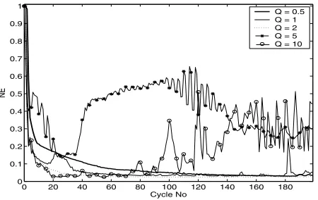
Figures 2 and 3 show results obtained for a sinewave and a repeating sequence demand. The total error incurred during each trial over the course of 200 iterations is plotted against the trial number in each case. The normalised error (NE) is simply the total error produced in a trial multiplied by a scalar chosen so that a constant zero plant output produces a NE value of unity. Without learning, a NE of 1 would constantly be incurred. Tests have been stopped if excessive vibration of the plant output makes it unsafe to continue, this can occur at fairly low levels of NE. Different values ofQ are used, the value ofR being fixed at unity. It can be seen that increasingQincreases the convergence speed but leads to large transients and divergence of error if set too high. The repeating sequence demand, which includes higher frequency components, exhibits slower con-vergence, greater transients, and a greater value of the minimum error. In both cases a value ofQ = 2produces good results. Figures 4 and 5 show similar results, but
0 20 40 60 80 100 120 140 160 180
0 0.1 0.2 0.3 0.4 0.5 0.6 0.7 0.8 0.9 1
Cycle No
NE
Q = 0.5 Q = 1 Q = 2 Q = 5 Q = 10
Fig. 2. Cycle error results for sinewave demand,N= 1
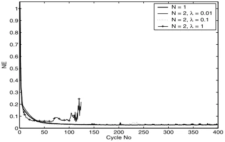
using a predictive horizon,N = 2. In this case the number of iterations performed has been increased to 400. Three values of λare used, each with two different values ofQ.
0 20 40 60 80 100 120 140 160 180 0
0.1 0.2 0.3 0.4 0.5 0.6 0.7 0.8 0.9 1
Cycle No
NE
[image:5.612.323.545.69.214.2]Q = 0.5 Q = 1 Q = 2 Q = 5 Q = 10
Fig. 3. Cycle error results for repeating sequence demand,N= 1
transients. This is expected since λdictates the amount of data used from the future trials. In practice the increase of λ produces a large change in u(t) at the beginning of each trial meaning that frequently tests must be discontinued due to the possibility of damage to the plant. This effect is due to the presence of a deadzone in the plant and occurs whether the plant output position is reset inbetween trials, or whether the next trial follows immediately on from the preceeding one. Figures 6 and 7 show the reference,
0 50 100 150 200 250 300 350 400
0 0.1 0.2 0.3 0.4 0.5 0.6 0.7 0.8 0.9 1
Cycle No
NE
λ = 0.01, Q = 1
λ = 0.01, Q = 5
λ = 0.1, Q = 1
λ = 0.1, Q = 5
λ = 1, Q = 1
λ = 1, Q = 5
Fig. 4. Cycle error results for sinewave demand,N= 2
input and output signals for the sinewave and repeating sequence demands respectively. These were recorded on the
400th cycle of the test which used the parametersN = 2,
λ = 0.1 and Q = 1. The demand is seen to be tracked accurately without excessive control action. Figures 8 and 9 compare results for varying amounts of prediction, using
Q= 1andQ= 5respectively. Only the repeating sequence demand is used and the N = 1 result is compared with the N = 2 used in conjunction with varying λ. It can be seen that prediction (N = 2) is capable of adding robustness to the algorithm with a suitable value ofλsince the error shows reduced transients and more trials can be performed before the tests are halted. Only a slight increase in convergence rate is evident from the experimental results. The following statements can hence be made concerning
0 50 100 150 200 250 300 350 400
0 0.1 0.2 0.3 0.4 0.5 0.6 0.7 0.8 0.9 1
Cycle No
NE
λ = 0.01, Q = 1
λ = 0.01, Q = 5
λ = 0.1, Q = 1
λ = 0.1, Q = 5
λ = 1, Q = 1
[image:5.612.69.294.72.214.2]λ = 1, Q = 5
Fig. 5. Cycle error results for repeating sequence demand,N= 2
0 1 2 3 4 5
−2 0 2 4 6 8 10
Time (s)
Output (rad) / Input (V)
[image:5.612.320.548.253.394.2]Demand, r(t) Output, y(t) Input, u(t)
Fig. 6. Signals at 400thcycle for sinewave demand,N= 2,λ= 0.1,
Q= 1
the design paramaters:
• Use of prediction can increase robustness
• The level ofQdictates convergence speed for a fixed
R but causes instability if excessively high
• The convergence of the repeating sequence demand is slower than for the sinewave demand
• Increasing the predictive horizon increases the conver-gence speed
• Increasingλcauses large input changes at the start of a trial
The bound on theH given by (23) does not provide useful information for the plant in question sinceσ2 is very large in this case. However using thel∞ norm in place of thel2 norm allows the approximation
σ2≈ 1
2 minw|G(w)|
(38) for the case that Q = R = 1, which is considered next. If the assumption is made that frequencies present in the demand dominate the learning process, then the bound on
0 1 2 3 4 5 −8
−6 −4 −2 0 2 4 6 8 10
Time (s)
Output (rad) / Input (V)
[image:6.612.66.293.71.214.2]Demand, r(t) Output, y(t) Input, u(t)
Fig. 7. Signals at 400th cycle for repeating sequence demand,N = 2,
λ= 0.1,Q= 1
0 50 100 150 200 250 300 350 400
0 0.1 0.2 0.3 0.4 0.5 0.6 0.7 0.8 0.9 1
Cycle No
NE
N = 1
N = 2, λ = 0.01
N = 2, λ = 0.1
N = 2, λ = 1
Fig. 8. Cycle error results for repeating sequence demand,Q= 1
sequence demand yieldsσ2= 0.56. For the case ofN = 1 these values, when inserted in (24), lead to convergence rates of l1= 0.44 and0.6 respectively, and Q= 1. These are close to the initial learning rates observed in practice. For the case of N = 2 the convergence rates for the two sequences becomel2= 0.443and0.64for λ= 0.01,l2=
0.43and0.625forλ= 0.1, andl2= 0.36and0.51forλ=
1. The convergence rates are plotted in Figure 10 for the repeating sequence. Comparison with the experimental rates seen in Figure 8 shows these theoretical bounds are accurate models for early trials. The lack of robustness with respect to high frequency modelling then reduce the learning rates significantly.
VII. CONCLUSIONS
Predictive Optimal ILC has been derived for discrete-time systems. The algorithm has been used on an experimental non-minimum phase spring-mass-damper system. Two val-ues of predictive horizon have been investigated. Excellent results have been achieved and the effect of parameter variation has been investigated. Practical implementational issues have been discussed and methods for increasing the computational efficiency have been proposed. The conver-gence rates observed have been compared to theoretical values.
0 50 100 150 200 250 300 350 400
0 0.1 0.2 0.3 0.4 0.5 0.6 0.7 0.8 0.9 1
Cycle No
NE
N = 1
N = 2, λ = 0.01
N = 2, λ = 0.1
[image:6.612.321.544.74.209.2]N = 2, λ = 1
Fig. 9. Cycle error results for repeating sequence demand,Q= 5
1 1.5 2 2.5 3 3.5 4 4.5 5 0
0.1 0.2 0.3 0.4 0.5 0.6 0.7 0.8 0.9 1
Cycle No
NE
N = 1 N = 2, λ = 0.01 N = 2, λ = 0.1 N = 2, λ = 1
Fig. 10. Theoretical convergence rates for repeating sequence withQ= 1
VIII. FUTURE WORK
The effect of varying the sampling frequency is a natural area of future study. The results presented here will also be compared with those achieved using the same algorithm on an industrial gantry robot. The algorithm robustness is an open area for further study.
REFERENCES
[1] K. L. Moore, “Iterative learning control - an expository overview,” Applied and Computational Controls, Signal Processing and Circuits, no. 1, pp. 151 – 214, 1998.
[2] ——, Iterative Learning Control for Deterministic Systems. Springer-Verlag, 1993.
[3] Z. Bien and J. Xu, Iterative Learning Control, Analysis, Design, Integration and Applications. Kluwer Academic Publishers, 1998. [4] N. Amann, D. H. Owens, and E. Rogers, “Iterative learning con-trol using optimal feedback and feedforward actions,”International Journal of Control, vol. 65, no. 2, pp. 277–293, 1996.
[5] ——, “Iterative learning control for discrete-time systems using optimal feedback and feedforward actions,” in Proceedings of the 34th Conference on Decision and Control, December 1995, pp. 1696–1701.
[6] ——, “Iterative learning control for discrete-time systems with ex-ponential rate of convergence,” inIEE Proceedings - Control Theory Applications, vol. 143, no. 23, March 1996, pp. 217–224.
[7] ——, “Predictive optimal iterative learning control,” International Journal of Control, vol. 69, no. 2, pp. 203–226, 1998.
[8] D. G. Luenberger, Optimization by vector space methods. John Wiley and Sons, New york, 1969.
[9] C. Freeman, P. Lewin, and E. Rogers, “Experimental comparison of extended simple structure ILC algorithms for a non-minimum phase plant,”Submitted to ASME, 2004.
[image:6.612.361.509.253.359.2] [image:6.612.66.292.259.402.2]