Optimization using surrogate models and partially converged computational fluid dynamics simulations

Optimization using surrogate models and

partially converged computational fluid

dynamics simulations

BY ALEXANDER I. J. FORRESTER*, NEIL W. BRESSLOFF AND ANDY J. KEANE

Computational Engineering and Design Group, School of Engineering Sciences, University of Southampton, Southampton SO17 1BJ, UK

Efficient methods for global aerodynamic optimization using computational fluid dynamics simulations should aim to reduce both the time taken to evaluate design concepts and the number of evaluations needed for optimization. This paper investigates methods for improving such efficiency through the use of partially converged computational fluid dynamics results. These allow surrogate models to be built in a fraction of the time required for models based on converged results. The proposed optimization methodologies increase the speed of convergence to a global optimum while the computer resources expended in areas of poor designs are reduced. A strategy which combines a global approximation built using partially converged simulations with expected improvement updates of converged simulations is shown to outperform a traditional surrogate-based optimization.

Keywords: computational fluid dynamics; data fusion; design of experiment; Kriging

1. Introduction

Computational fluid dynamics (CFD) can have the largest impact on aircraft design by its inclusion in the conceptual design process. This is the stage where important design configuration decisions are made and global optimization can play a key role. After the conceptual stage, the design process is based increasingly on local optimization to fine-tune the design. Currently, most optimization at the conceptual stage is carried out using empirical design tools based on previous aircraft and engineers’ experience. These tools may be unable to predict the behaviour of radical geometries at this, the only, point in the design process where they may be considered seriously (Giannakoglou 2002). Thus, a key challenge is to be able to perform global optimization using physics-based simulations in an efficient manner, so as to allow these methods to be used within the short time-scales of conceptual design.

Published online6 March 2006

* Author for correspondence ([email protected]).

This work concentrates on the use of surrogate models1 in optimization (Box & Draper 1987;Schonlau 1997;Jones 2001), which are used in lieu of direct calls to a CFD code. A global surrogate model, of the drag of an aircraft for example, is not as accurate as individual simulations, but gives almost instantaneous results allowing exhaustive global searches to be performed. This meta model must first be built using a number of initial simulations defined by a design of experiment (DoE). Commonly, when dealing with a global model, there is no prior knowledge of the shape of the objective function landscape, and so the same amount of computing effort is normally applied in all areas via the even distribution of the initial simulations throughout the design space. Significant time savings could be achieved if more effort were directed at finding the optimum rather than modelling regions of poor designs. This is, of course, the logic of purely local models, but they forgo any wider exploration of radical designs. An optimization design space with widely set bounds (to encompass radical designs) can be searched effectively using local methods if the design space is uni-modal, i.e. there is only one basin of attraction for the search to descend into. However, it must be assumed that there may be many local basins of attraction—the probability of this increasing along with widening the bounds and increasing the dimensionality of the design space. Thus, a global search is required to increase the chances of isolating the global optimum.

The literature contains a number of examples of previous attempts to direct more high-fidelity (physics based) design evaluation at promising designs within a global optimization environment.Masonet al. (1998)present a review of work on the conceptual design of a high speed civil transport (HSCT) aircraft, in which DoE, variable complexity analysis using the ‘reasonable design space’ approach (Balabanovet al. 1999), and polynomial response surface modelling are used to incorporate high-fidelity analysis into conceptual design.Knillet al. (1999)make use of the same HSCT problem to investigate using a low-fidelity model to decrease the number of terms used to build a polynomial RSM and so reduce the number of high-fidelity simulations required. The University of Southampton multi-level wing design environment (Keane & Petruzzelli 2000) attempts to combine the merits of varying fidelity computer models in the conceptual design of a commercial airliner wing. A more exhaustive search can be performed using a quick empirical code (Tadpole;Cousin & Metcalf 1990) than is feasible with a more expensive Euler code, so an extensive search using the empirical code is used to seed a narrower search using Euler simulations. The wing design environment is used again by Keane (2003) to evaluate the use of data fusion (Vitaliet al. 1999;Alexandrov et al. 2001) in wing design. Computation time is dramatically reduced while the accuracy of the two computer models is combined to give a better optimum than either code in isolation.

The above methods have relied on the availability of a suitable low-fidelity model for a preliminary evaluation of the design space. Often this model will be empirically based and may not be applicable for new areas of research or radical designs. In contrast to the above strategies, this paper investigates methods for improving the efficiency of optimization through the use of partially converged CFD simulations using a high-fidelity physics-based code. These allow surrogate

1

models to be built in a fraction of the time required for models based on converged results. Such surrogates will be applicable in areas outside of the domain of empirical models and may be able to identify possible radical designs (should a suitable correlation between partially and fully converged simulations be achieved). No separate low-fidelity model is required and the same physics-based model is used throughout the optimization process. In essence, we propose that partially converged high-fidelity simulations are used as a low-fidelity model in a multi-level environment.

Using partially converged results in optimization is not an entirely new idea. Kuruvila et al. (1995) make modifications to the geometry based on gradient information from an adjoint solution (Jameson 1988) at stages throughout a multi-grid cycle to arrive at an optimal design for the cost of approximately two to three CFD solutions. Gumbert et al. (1999) pause a simulation to make changes to the geometry, again based on gradient information. The partially converged simulation is then interpolated onto a new grid and the procedure repeated until convergence, at which point an optimal design is achieved. Reported costs range from 15 standard simulations for a two variable optimization to 130 for eight variables. Dadone & Grossman (2003) use a similar method, but also refine the computational mesh as the solution progresses. The dependence of these methods on gradient information rather than objective function values means that only local optimization through gradient descent methods is possible.2 Such methods are unsuitable for use with direct global optimization routines such as a genetic algorithm or a dynamic hill climber, since the convergence would have to start from scratch at each restart. Of course, multiple restarts are possible, but this will naturally increase the computational expense. Further work in this area is reported by Newman et al. (1999).

The techniques described above take advantage of gradient information and, furthermore, that this gradient takes approximately the correct value at an early stage in the convergence of the simulation. Thus, the direction an optimization process should take is known before the final objective function value is converged. By thinking in terms of surrogate models, this characteristic of the convergence of CFD simulations can be utilized to enhance the efficiency of global optimization: if the gradients of individual simulations take approximately the correct value early in convergence, it follows that the shape of a surrogate built from a number of partially converged simulations will already have taken on a useful form. The surrogate may not be accurate in regions of near zero gradient, but promising areas are likely to have been revealed. This evolutionary characteristic of partially converged surrogate models has been demonstrated by Forrester et al. (2003). The partially converged surrogate model can be used in lieu of other low-fidelity models within a multi-level or data fusion based approach, and so enables high-fidelity CFD simulations to be used in conceptual design, thus combining the benefits of partially converged data, previously exploited in local optimization, with global response surface techniques.

2_{Gradient-based search, if the gradients are able to be computed efficiently, e.g. through an adjoint}

This paper examines the number of simulations and the level of convergence necessary to perform such optimization. Methods are investigated for determining when satisfactory convergence has been reached and also if the design space has been sampled sufficiently. Section 2 applies traditional surrogate-based optimization to an example problem for use as a comparison with methods outlined in further sections. Section 3 discusses, and presents results in answer to the question: ‘how many designs should the initial DoE comprise and to what extent should the simulation of these designs be converged?’ Section 4 describes and demonstrates an optimization scheme based on the results from §3, while §5 presents and demonstrates a possible optimization method for the scenario of there being no prior knowledge of the problem. This method is then applied to a more complex and time-consuming wing design problem in §§6 and 7, with extension to further complexity and increases in dimensionality discussed in§8. Finally, conclusions are drawn in§9.

2. Traditional surrogate model-based optimization

The use of surrogate models in optimization is becoming increasingly popular and we begin this section with a short introduction to the process. The surrogate model is not in itself an optimizer, but rather a tool for increasing the speed of optimization. Instead of making direct calls to an expensive computer code, an optimization routine takes values from a cheap surrogate model of it.

The popularity of such methods has probably increased due to the development of surrogate model based methods, which are better able to capture the nature of a multi-modal design space. Low-order polynomials (Box & Draper 1987) are notorious for predicting erroneous optima of complex functions, while the more advanced method ofKriging3(Sackset al. 1989;Cressie 1989) has been shown byJoneset al. (1998)(in a refreshingly transparent manner) to be a robust, though complex method able to predict even the most deceptive of global optima.

geometry parameterization

construct RSM

DoE search

RSM

design

adequate? optimum_design yes

CFD

no

update stage one

CFD

CFD _CFD

CFD _CFD

CFD _CFD

stage two

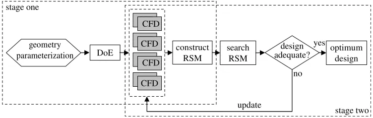
Figure 1. Two-stage surrogate model-based optimization strategy.

3_{So called byMatheron (1963)after D. G. Krige—a South African mining engineer who developed}

the method in the 1950s for determining ore grade distributions based on core samples (Krige

This paper is limited to the so-calledtwo-stageapproach (as defined byJones (2001) and depicted infigure 1), where, in the first stage, a surrogate model is built on the basis of a number of function evaluations (chosen on the basis of a DoE), before a search and update strategy is performed on the surrogate in the second stage. Each update simulation enhances the accuracy of the surrogate model in areas of promising designs. This process is iterated until the optimum of the function is found or a stopping criterion is met. This search and update strategy is demonstrated here via its application to the optimization of the shape of an aerofoil.

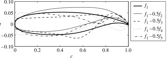
The aerofoil is defined by five orthogonal shape functions (Robinson & Keane 2001) and a thickness to chord ratiot=c. The first function, which represents the shape of a NASA supercritical SC(2) aerofoil (Harris 1990), and t=c are kept constant (t=cis fixed at 10%). The first function,f1, is in fact a smooth least-squares fitting to the coordinates of the SC(2) series of aerofoils. Each of the four subsequent functions,f2;.;5is a least-squares fitting to the residuals of the preceding fit, and can be added tof1with a greater or lesser weighting,wi, in order to vary the aerofoil geometry.Figure 2 shows the effect of adding each function with a weighting of

wiZK0:5 tof1. Nonsensical aerofoils are produced by adding individual functions

with such large weightings, but a high degree of geometry control is achieved by combining the functions and optimizing their weightings.

The drag coefficient (CD) of the aerofoil is to be minimized subject to a fixed lift constraint, CLZ0:6, at free-stream Mach number, MNZ0:73 and standard

atmosphere conditions at 10 000 m. The drag is calculated in the commercial CFD solver FLUENT (Fluent 2003) using surface pressure integration over the aerofoil. This is not necessarily the most accurate way to calculate the drag (Levy et al. 2002), but is used throughout this paper and so results are directly comparable with each other. Euler simulations are performed on unstructured meshes of approximately 13 000 triangular cells. Studies performed show that the mass continuity converges to 10K6 _{after 2500 iterations, but that the force}

coefficients remain constant (G0:1 drag counts) after 1500 iterations. Since it is the force coefficients that are used as a figure of merit for optimization, simulations run for 1500 iterations are deemed to be, and referred to in this paper as, ‘fully converged’. The use of this aerofoil optimization as an example problem enables quick evaluation of designs using two-dimensional inviscid transonic flow simulations (approx. 5 min per simulation), allowing optimization methodologies to be examined without the hindrance of lengthy computation times.

0 0.2 0.4 0.6 0.8 1.0

– 0.10 – 0.05 0 0.05 0.10

c t

f₁

f₁ – 0.5f₂ f₁– 0.5f₃

f₁– 0.5f₄ f₁– 0.5f₅

The constant lift constraint is maintained by varying the angle of attack (a) of each aerofoil. At low to moderate values ofa, i.e. before flow separation and stall,CL varies linearly witha. The first aerofoil geometry is simulated at an initially guessed a1, and at a2 determined by the result of the first simulation and an estimate of

DCL=Da. A third simulation at a3, found from a linear interpolation through (a1,CL1) and (a2,CL2), is sufficient to attain the desired lift and an accurate value of

DCL=Da. Subsequent geometries are simulated usinga1and CL1 from the closest previously computed aerofoil, in terms of the Euclidean distance between variables, such that, after the first few geometries, it is rarely necessary to proceed further than a2before the desired lift is met to within 1%.4

An initial set of 10 designs chosen by an LPt DoE (Sobol 1979; Statnikov & Matusov 1995) are simulated before constructing a Kriging model of the expected improvement (Schonlau 1997) in the objective function (the hyper-parameters of which are selected by a maximization of the likelihood of the DoE data using a genetic algorithm and dynamic hill climber; e.g.Keane & Nair 2005)—stage one infigure 1 (a straightforward and intuitive description of Kriging and likelihood is presented byJones (2001); see also Sacks et al. 1989). The number of initial simulations is chosen rather arbitrarily, since there is no clear consensus in the literature as to how many points should be used.Joneset al. (1998)suggest 10 points for every dimension, whileSo´besteret al. (2005)indicate that one-third of the total number of simulations available (dictated by time or cost) should make up the initial sample. This issue will be addressed further in§3. Although an optimal Latin hypercube DoE (Morris & Mitchell 1995) produces a more even space filling design than the LPtmethod, the latter is attractive (particularly for use in future sections of this paper), since subsets taken from a larger LPtDoE are, in themselves, space filling. The same DoE method is used throughout so as to maintain comparability of results.

C_D

C_D data minimum C_D

0 5 10 15 20 25 30

0.016 0.017 0.018 0.019 0.020 0.021 0.022

number of designs

variation across 5 DoEs

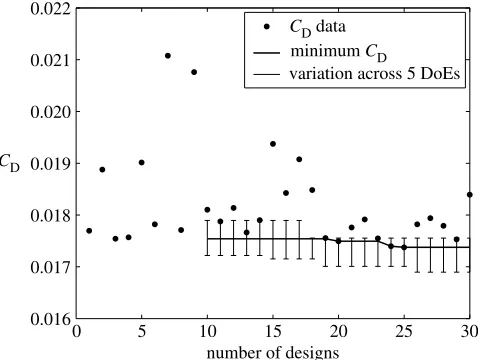
Figure 3. Expected improvementCDoptimization history starting from a 10-point LPtinitial DoE

(using Kriging interpolation).

4

Equality constraints are difficult to handle when using surrogate models. The procedure outlined here effectively removes theCLconstraint from the optimization by making it a condition which

Following the initial DoE, a new simulation is performed, and desired lift attained, for an aerofoil defined by variables that maximize the expected improvement inCD. This simulation is then added to the Kriging model and the process continues, as per stage two in figure 1.

The objective function history is shown infigure 3, where the minimumCD is plotted against the number of designs that have been evaluated (the first 10 being from the initial DoE). The individualCD values for each aerofoil shape are also shown and, in order to display the degree of dependence on the initial DoE, error bars indicate the range of values obtained from five independent optimizations using a series of random Latin hypercube DoEs. This form of surrogate-based optimization represents the current practice in many major aerospace companies and as such is used as a basis for comparison with methods discussed in subsequent sections of this paper. Of course, the Euler calculatedCD does not necessarily represent the true drag characteristic of the aerofoil and the results are suitable only for comparison with similarly computed CD values.

3. Building the initial dataset

A sensible location at which to position an update simulation, i.e. the combination of design variables which will lead to an improved objective function, is chosen on the basis that the objective function has been adequately approximated by the surrogate model. The initial DoE must contain sufficient data, in terms of both quantity and quality (accuracy of data), to build an effective surrogate model in order to allow further computing effort to be directed at optimal regions of the design space. Too much data (either quantity or quality) will lead to wasted effort in sub-optimal areas, since the initial DoE is constructed so as to give an even spread of data throughout the domain of interest. Too little data may result in erroneous predictions of optimal regions with poor positioning of update simulations as a consequence.

(a) Determining the quality of a surrogate model

The quality of a surrogate model can be assesseda posterioriby comparing an independent set of objective function data with values taken from the surrogate at points corresponding to the variables at which the independent objective function values are calculated, i.e. exact data is compared with approximate data. The data is compared using the correlation coefficient or coefficient of determination,r2 (Edwards 1976):

r2_Z s_{ffiffiffiffiffiffiffiffiffi}ff^

sfs_f^ p

!2

Z N

P

ff^KPfPf^

ffiffiffiffiffiffiffiffiffiffiffiffiffiffiffiffiffiffiffiffiffiffiffiffiffiffiffiffiffiffiffiffiffiffiffiffiffiffiffiffiffiffiffiffiffiffiffiffiffiffiffiffiffiffiffiffiffiffiffiffiffiffiffiffiffiffiffiffiffiffiffiffiffi

½NPf2Kð P

fÞ2½NP^f2Kð P_^

fÞ2

q 0 B @

1 C A 2

; ð3:1Þ

where N is the number of results to be compared, f denotes objective function values from the independent test set and ^f are approximate objective function values taken from the surrogate at the locations off. If the correlation is equal to 1, the surrogate is exactly predicting the test data, while r2_Z0 indicates no correlation between the surrogate and the objective function.

(Myers & Montgomery 1995).5 However, it will be seen that this is not an appropriate method for assessing the majority of surrogate models considered in this paper.

In the following sections, r2 is calculated using objective function values of

L=D instead of CD since, although as a post-process it is possible to use CD results from simulations that meet a fixed lift criterion, it is impracticable to do so at early stages of convergence during the process of performing surrogate model updates (as is done later in this paper). AsL=Dis directly related to both

CLandCD, it is assumed that a good correlation inL=Dindicates that a similarly accurate model may be produced for CD at a fixed CL.

(b) DoE size

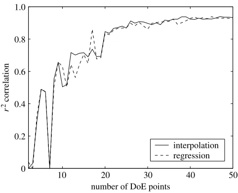
The initial surrogate model in the previous example had a correlation coefficient of r2_Z0:5215 when compared to 10 independent simulations from an optimal Latin hypercube DoE (not shown): far from an exact representation of the objective function and inappropriate for the selection of update points—as demonstrated by the lack of improvement inCDimmediately following the initial DoE seen in figure 3. It takes 10 further simulations before an improvement is made on the lowest DoE value. It is expected that the quality of the surrogate would diminish with fewer DoE points and increase with a greater number. This assertion is tested by comparing surrogate models built using varying numbers of points from the LPt DoE with the 10-point optimal Latin hypercube dataset. The resultingr2plot is shown infigure 4. Note that at 10 points, the LPtDoE is the same as that used in the previous example and so the correlation is identical.

10 20 30 40 50

0 0.2 0.4 0.6 0.8 1.0

number of DoE points

r

2 correlation

interpolation regression

Figure 4.r2correlation versus number of points in the LPtDoE.

5

The correlation is indeed poor when using a small DoE, with a dramatic drop in surrogate model quality when fewer than eight points are used. The surrogate becomes erratic due to the Kriging model being unable to fit such a sparsity of data: one model, with one set of hyper-parameters, produces a similarly poor likelihood of the data as another model with another set of hyper-parameters. The correlation improves as more points are added, though there is little to be gained by using an initial DoE with greater than 20–25 points. At this stage,

r2levels off and further addition of points does not globally improve the surface,6 although the accuracy of the surface in the region immediately surrounding an added point is likely to be enhanced.

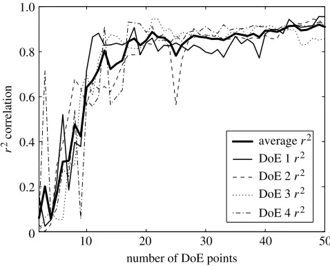
These observations of the effect of DoE size are not unique to the DoE which has been chosen. DoE independence is shown by averaging the correlation obtained for four surrogate models built from independent random Latin hypercubes. These correlations are shown in figure 5. The same test data of 10 optimal Latin hypercube points have been used. It is seen that r2 is largely unaffected by the choice of DoE for this problem. The averaging means that the correlation is slightly less erratic than that shown infigure 4, but a similar trend is seen between both plots.

The notion that increasing the number of DoE points increases the accuracy of the surrogate model is rather straightforward, but here we have shown that there is a limit beyond which adding more points gives minimal return in terms of increasing surface accuracy. We now go on to discuss the main thrust of this paper, which is the use of partially converged simulations to build surrogate models.

10 20 30 40 50

0 0.2 0.4 0.6 0.8 1.0

number of DoE points

r

2 correlation average r2

DoE 1 r2

DoE 2 r2

DoE 3 r2

DoE 4 r2

Figure 5.r2versus number of points for four random Latin hypercube DoEs.

6

The correlation fails to reach a perfect value of 1, not only because a surrogate model can never

preciselymatch the true function, but also due to the noise in the data from varying discretization error caused by changes in the mesh as the aerofoil shape alters. However, it is seen infigure 4that regressing the data leads to no improvement in the correlation—indicating that it is noise in the test data that is producing the lack of correlation. This subject is considered in more depth by

(c) Simulation convergence

The r2 correlation indicates whether the surrogate model’s shape is accurate, but is unaffected by global changes in the magnitude of the objective function. Surrogate models built using the original 10 simulations at stages throughout their convergence are in fact still correlated with the converged 10-point optimal Latin hypercube dataset (as previously demonstrated byForresteret al. (2003)). Note that a leave-one-out cross-validation on a partially converged surrogate would simply show how well the surrogate is approximating the partially converged data it is built from and provide no indication of the quality of the surrogate model in terms of the converged design space.

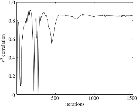
The r2 correlation history throughout the convergence of a surrogate built with 50 partially converged simulations is shown in figure 6, while the L=D

convergence history for the mean aerofoil (defined by just the first basis function and t=c, withw2;.;5Z0) is displayed infigure 7. It is seen that the shape of the design space is approximated successfully long before L=D has reached a stable value, with r2Z0:8 after just 80 iterations. This indicates that the surrogate

model assumes a characteristic shape early in the convergence of the CFD and experiences mean shifts as the simulations progress. Note that while a consistent value of a force coefficient from iteration to iteration must be seen before a simulation is considered converged, an individual high r2 value indicates that the surrogate model is accurate in terms of its shape. It is argued here that the position of update points could therefore be selected at a very early stage in the iterative process of CFD simulations. However, caution is required since significant irregularity can occur in the convergence of bothr2and the objective function—as observed, for this example, infigures 6 and 7between 220 and 290 iterations. Inspection of the flow over the baseline geometry reveals that the iterative simulation produces a large area of supersonic flow at this stage, with associated dramatic changes in pressure, before reverting to largely subsonic flow.Figure 8shows a large pressure drop behind this area of supersonic flow (at 200 iterations), moving forward (250 iterations) and approaching the position of

500 1000 1500

0 0.2 0.4 0.6 0.8 1.0

iterations

r

2 correlation

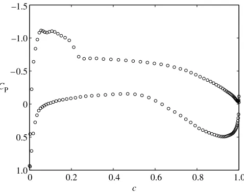
the shock predicted by the converged simulation (300 iterations) in phase with the irregularities in convergence seen in figures 6 and 7. Figure 9 shows the converged CP, with a small region of supersonic flow towards the front of the aerofoil followed by a shock and a more gradual compression over the aft upper surface. Not all geometries experience this irregularity to the same extent and of those that do, it occurs at slightly different stages in the simulation. This phenomenon naturally has a large impact on the predicted force coefficients and, in doing so, affects the development of the surrogate model. Up to this point, and indeed later in the convergence history, the surrogate model accurately predicts the smooth and continuous manner of the objective function, but the introduction of discontinuities cannot be modelled effectively by a global surrogate.

500 1000 1500

0 10 20 30 40 50

iterations

L

/

D

Figure 7.L/Dconvergence history for the baseline aerofoil.

0 0.2 0.4 0.6 0.8 1.0

–1.5

–1.0

–0.5

0

0.5

1.0

1.5

c C_P

200 iterations 250 iterations 300 iterations

(d) Optimum DoE size and simulation convergence

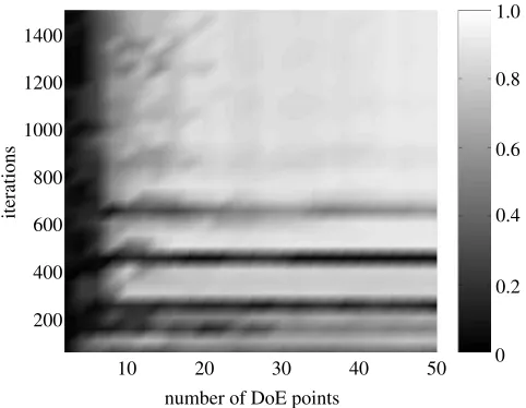
For the aerofoil optimization example studied here, it has been shown that there is an optimum number of initial DoE points and a minimum number of iterations for which these should be simulated to produce an accurate representation of the shape of the objective function for minimal cost. These two variables are plotted against each other in figure 10 to show how they together affect the quality of the resulting surrogate model of the four variable aerofoil optimization problem. The same trends are present here as in figures 4

–1.5

–1.0

– 0.5

0

0.5

1.0

C_P

0 0.2 0.4 0.6 0.8 1.0

c

Figure 9. Converged CP(after 1500 iterations) (CLZ0.7).

1400

1200

1000

800

600

400

10 20 30 40 50 0

0.2 0.4 0.6 0.8 1.0

number of DoE points 200

iterations

a

b

Figure 10.r2_{for varying number of DoE points and number of iterations. The dashed line shows}

and 6, including the large drops in correlation due to irregularities such as those seen in figure 8. These trends could be a characteristic particular to the LPt DoE, but this notion is dispelled by figure 11, which is constructed using the average correlation of surrogate models built using four independent random Latin hypercube DoEs.Figures 10 and 11are in fact almost identical, indicating that the trends are independent of the choice of DoE.

Bothfigures 10 and 11show clearly that a small initial DoE of fully converged simulations will lead to a poor surrogate model. A greater number of DoE points produces a more accurate surrogate model, even if the simulations are not fully converged. It is suggested that, for an equivalent computing effort, a more efficient optimization can be performed than the earlier example if the initial DoE comprises a greater number of partially converged simulations. If computing effort is defined simply as ‘number of iterations!number of design points’ then the dashed line in figure 10represents a line of constant computing effort equivalent to that used to produce the initial 10 DoE points for the earlier example optimization, i.e. 1500!10. Point ‘a’ depicts the fully converged 10-point DoE, while point ‘b’ indicates the position on the line of constant computing effort which represents the highest correlation with the 10 independent converged simulations. This indicates that a surrogate model built with 26 simulations converged to 575 iterations is the most accurate surrogate model which can be produced for the given computing effort.

4. Optimization using partially converged simulations

We now present a strategy for utilizing a surrogate model built from partially converged simulations, such as the optimum DoE derived fromfigure 10, within a surrogate model-based optimization. But first, the issue of meeting constraints, such as the lift constraint applied in the aerofoil optimization, must be addressed.

1400

1200

1000

800

600

400

200

iterations

10 20 30 40 50

number of DoE points

0 0.2 0.4 0.6 0.8 1.0

It is not possible to meet a fixed lift criterion, or indeed any other simulation-based constraints, with partially converged results, since the force coefficient values have not reached their true value. However, if it is assumed that all designs undergo an equal shift in the value of CL between intermediate iterates and their final converged value—an assumption based on the high correlations in L=D seen in §3—we can use a single converged result to scale all other designs. a can then be adjusted for each design to meet the required lift criterion. Since, when performing CFD analysis, it is usually necessary to compute at least one test simulation to check the mesh and solution setup, this simulation can take the form of the first point of the initial DoE and be used to scale all further simulations. While a mean shift relation between iterates is sufficient in this case, more complex properties for constraint quantities could be handled using the more complex correction strategy employed for the objective function—described in the remainder of this section.

We propose the use of fully converged update simulations at points of maximum expected improvement in order to enhance the accuracy of the global partially converged model in areas of promising designs. Applying converged updates to a partially converged surrogate model means that the optimization takes the form of a multi-level approach (e.g. Keane & Petruzzelli 2000), where a low-fidelity model is used to seed a search using a high-fidelity code. Usually, in direct optimization methods, the search using the low-fidelity model simply provides a starting point for the more expensive high-fidelity search before being discarded. In this instance, using a surrogate model-based method, information from the partially converged results is retained since they provide the data from which the initial surrogate model is built. The partially converged data, fpartðxpartÞ, is corrected using a difference approximation, f^diff, based on fully converged updates, fconvðxconvÞ, where

xconv3xpart. This results in a fused surface which benefits from the global surrogate afforded by the space filling partially converged simulations and local accuracy in optimal areas gained from the converged update points:

^

process quickly converges on the optimum of the true function. Minimal effort has been expended sampling regions of poor objective function values with fully converged simulations, although the first converged design cannot, of course, be positioned in an optimal region without prior knowledge of the design space—here we have simply taken the centre of the domain as the starting point, but a known good design is likely to speed up the process and provide improved constraint approximations in the optimal area.

This one variable example demonstrates visually the methodology in question, but it should be remembered that functions are rarely so simple in a multi-dimensional design space. Greater differences between partially and fully converged results are inevitable and more complex difference approxi-mations, requiring greater numbers of training points, are likely to be required. This method of applying data fusion to the evolving surrogate model (which we will for the remainder of this paper refer to by the more succinct term ‘evofusion’) differs from a standard multi-level optimization in that the low-fidelity simulations are retained for use in the high-low-fidelity optimization and it is not a standard form of data fusion, since there is no initial high-fidelity DoE from which to produce a global difference surface, i.e. more of the expensive simulations are now directed at regions of promising designs.

0.02 0.03 0.04 0.05

C_D

0.02 0.03 0.04 0.05

C_D

0.02 0.03 0.04 0.05

C_D

start

true C_D function part converged RSM part converged points difference RSM (+0.02) difference points (+0.02) fused RSM

fused points converged points

1 update

2 updates

– 0.3 – 0.2 – 0.1 0 0.1

w₂

– 0.3 – 0.2 – 0.1 0 0.1

w₂

3 updates

4 updates

(a) Partially converged surrogate model update example

In light of the results presented infigure 10, the first 26 points of the LPtDoE converged to 575 iterations are now used as the starting point to demonstrate the application of the strategy outlined in §3 to the four variable aerofoil optimization problem. Figure 13shows the optimization history of the evofusion method alongside the baseline fully converged method described in §2. CD is plotted on the y-axis and the total number of iterations performed, including those needed to reach the fixed lift criterion, is shown on the x-axis.

As seen in figure 13, the evofusion strategy consistently outperforms the traditional optimization throughout the update history. Note that there are fewer updates with high CD values when using the evofusion method. Here the traditional strategy is sampling sparsely populated areas of poorly performing designs, whereas the larger partially converged DoE has already explored these areas—highlighting them as sub-optimal regions—and clusters updates in more promising areas. Results for both the LPt based, and the average performance across the random Latin hypercube based, traditional and evofusion optimiz-ations are presented in table 1. The quality of, and iterations required to build, the initial DoE are shown (including the iterations required to meet the CL criterion, which is why the 26-point partially converged DoEs actually require more iterations than the 10-point converged DoEs), as is the optimizedCDalong with its percentage improvement over the baseline NASA aerofoil. The time limit for these optimizations is based on the time taken for the traditional 10-point LPt DoE plus 20 updates. It is seen that the improvement over the baseline design when using the evofusion method is on average 80% better than for the traditional optimization. Results are also included for LPt DoE based optimizations at

C_D

traditional C_D data traditional minimum C_D variation across five DoEs evofusion C_D data evofusion minimum C_D

variation across five DoEs

0 2 4 6 8 10

0.016 0.017 0.018 0.019 0.020 0.021 0.022 0.023 0.024

total iterations (× 104)

a fixedCLof 0.7 (using the same initial DoEs as theCLZ0:6 cases). Similar drags are achieved with both methods, although the evofusion method is 30% faster.

5. Real time surrogate model quality assessment

The optimizations performed in §4 took advantage of prior knowledge attained (fromfigure 10) at the expense of a large amount of computing effort. However, it is infeasible to compute a test set of fully converged simulations when performing optimization in an industrial environment. A real time method of surrogate model quality assessment is required to take advantage of possible time savings afforded by using partially converged simulations.

Rather than correlating values taken from a partially converged surrogate model with fully converged test data, it is possible to correlate partially converged surfaces with one another. The correlation rm2 of one surface with a

surface built using simulations converged formfewer iterations is an indication of the stability of the surrogate model. A low correlation indicates that the surface has changed significantly over the m iterations: the simulations are converging independently of each other causing the surrogate model to be in a state of flux. A high correlation indicates that the shape of the surface has changed little over them iterations, i.e. the simulations are converging in unison.

It can also be determined whether the size of the DoE is sufficient by correlating the surface in question with a surface built usingn fewer points. For n_Z1, this is similar to a leave-one-out cross-validation, but in this case it is an

add-one-invalidation. A high correlation indicates that the surface is unaffected Table 1. Aerofoil optimization performance comparison.

CLZ0.6 (baselineCDZ0.0177, minimum foundCDZ0.0166)

method

initial DoE best after 1.17!105iterations

r2 e(x)a its.b CD imp. (%) after: (its.)

10-pt LPtconverged 0.5215 0.4910 31 500 0.0174 1.7 96 000 10-pt converged avg. 0.4282 0.6409 34 800 0.0172 2.8 78 600 26-pt LPtevofusion 0.9065 0.4478 31 975 0.0173 2.3 108 475 26-pt evofusion avg. 0.8980 0.4718 45 775 0.0168 5.1 101 275

CLZ0.7 (baselineCDZ0.0249, minimum foundCDZ0.0211)

method

initial DoE best after 1.17!105iterations

r2 e(x)a its.b CD imp. (%) after: (its.)

10-pt LPtconverged 0.5215 0.6758 31 500 0.0219 12.1 88 500 26-pt LPtevofusion 0.9065 0.3900 45 775 0.0220 11.7 62 275

a

Euclidean distance of predicted optimum from best optimum found in this work (found using the evofusion method), with variables normalized between 0 and 1.

b

by the addition of new points, while a low correlation tells us that more points are needed to produce a good surrogate.

We now have a combined correlation of r_ð2_m;nÞ, to which we add a degree of robustness by averaging over l successive correlations to give

r2l

ðm;nÞZ1 l

Xl

iZ1

r_ð2_i!m;i!nÞ: ð5:1Þ

In§4, updates were applied to the optimum initial DoE for 15 000 iterations of total computing effort. Referring again tofigure 10it is seen that a high quality initial DoE can be computed for a greatly reduced computational cost. A clearer picture is seen by zooming in on the lower edge offigure 10to producefigure 14. This clearly displays regions of high correlations where the DoE size and iteration count shown could be used to build accurate approximations of the shape of the converged design space at minimal cost. There are also regions where the partially converged design space is an exceedingly poor representation of the converged data. A real time quality assessment must highlight not only the regions of high quality models, but also areas of poor models. Figure 14 is reproduced in figure 15, but this time using r23

ð5;1Þ, i.e. an average of rð25;1Þ, r 2

ð10;2Þ and r 2 ð15;3Þ. Although not an exact representation of figure 14, figure 15 correctly captures areas of consistently good and bad surrogates. For more insight into the formulation of this correlation criterion, the reader is directed toForrester (2004).

(a) Real time update scheme

To perform an efficient optimization using a surrogate model, it is necessary that a sufficient number of designs are simulated for the objective function to be accurately predicted before updates are applied, and, by referring tofigure 14, it is seen that these simulations should be limited to a certain number of iterations to avoid unnecessary time being devoted to poor designs. As more points are

0 0.2 0.4 0.6 0.8 1.0

10 20 30 40 50

number of DoE points 140

120

100

80

60

40

20

iterations

added, more accuracy is possible through increasing the number of iterations. This relationship between DoE size, number of iterations and surrogate model accuracy can be exploited through an update strategy which effectively drives the optimization diagonally from the bottom left corner offigure 14towards more DoE points and higher numbers of iterations in an intelligent manner.

A possible update scheme is now suggested that requires limited prior knowledge of the optimization to be performed. This scheme (i) uses the smallest possible initial space filling DoE, (ii) converges the CFD simulations to the minimum extent and (iii) adds converged expected improvement points as soon as possible.

The process is described via the flowchart in figure 16. First, a small, though larger thanl!n(we require this many points to compute the first moving average correlation overlsurfaces), initial DoE is converged form!literations, except for the first design which is fully converged. The multiple ‘CFD’ boxes infigure 16 denote that these simulations may be run in parallel, both in terms of a single simulation being run on a number of processors, and a number of different designs being run concurrently. If ther2l

ðm;nÞcorrelation does not meet a specified criterion, nnew designs defined by variables at the maximum error in the surrogate model are added to the DoE. This is equivalent to increasing the size of the DoE whilst maintaining its space filling characteristic. This could also be performed by increasing incrementally the size of an LPtDoE, but the use of maximum error as an infill criterion permits the use of a better space filling initial DoE, such as an optimal Latin hypercube. All designs are now simulated for a furthermiterations. The process continues until the r2l

ðm;nÞ criterion is met. This represents the end of stage one of the traditional two-stage surrogate-based optimization process.

At this point, the DoE is augmented by designs defined by variables at the maximum expected improvement of the surrogate model. The simulations of these update designs are fully converged and the right-hand side of the flowchart infigure 16 demonstrates how these are embedded within a two-stage

140

120

100

80

60

40

20

iterations

10 20 30 40 50

number of DoE points

0 0.2 0.4 0.6 0.8 1.0

Figure 15.r23

surrogate-based optimization system. These converged updates are fused to the optimum initial DoE, as described in §4, until a stopping criterion is met.

To construct a meaningful real time representation of the quality of a surrogate model usingr2l

m;n, it is necessary thatmandnare chosen prudently. In

essence, these parameters determine the gradient of a space filling update path moving diagonally through figure 14. mZ5 is seen to be appropriate for the

optimizations demonstrated here, although simulations that require far greater or fewer iterations, as determined by an initial test simulation, would benefit from a larger or smaller value of m.

stage one stage two

geometry parameterization

yes

l r2_{(m, n)}

criterion met? construct RSM using partially converged data

DoE

Search E[I(x)]

stopping criterion met?

optimum design yes

no no

search RSM error

calculate difference between partially and

fully converged data

construct RSM of difference

get difference predictions for all partially converged

data

correct partially converged data

construct fused RSM one fully converged

CFD simulation CFD

CFD

CFD CFD

part converged CFD

fully converged CFD CFD

CFD CFD

CFD CFDCFD CFD CFD CFDCFD

N–1 part converged CFD simulations

This paper has dealt purely with sequential updates to the surrogate model and so n should naturally be equal to one. If the benefits of parallel processing are to be utilized by updating the surface with a number of points at a time (So´bester et al. 2004), n might be increased in line with the number of parallel update points. Increasingn will provide a more robust stability criterion, hence CPU time is likely to increase, although increasing the number of parallel jobs will naturally reduce the wall clock time associated with this increased CPU time.

6. Three-dimensional wing optimization

The Euler simulations of two-dimensional aerofoils performed throughout this paper take approximately five minutes to fully converge when run on a single 2 GHz AMD processor. Computing three-dimensional flow demands significantly longer run-times. Here, six hours are required across four 2 GHz AMD processors with 100 Mb sK1 _{interconnect (24 CPU hours) for the convergence of an Euler}

simulation of a three-dimensional wing. As such the early identification of promising designs and elimination of poor designs is paramount.

The wing geometry is defined by 10 parameters, the first six of which describe the planform and are kept constant for this study at values appropriate for a generic 200 seat aircraft (areaZ200 m2, aspect ratioZ8, spanZ40 m, kink

positionZ0.4, sweepZ308, inboard taper ratioZ0.5 and outboard taper ratioZ

0.3), while the remaining four comprise the w2 basis function weighting of the root, kink, and tip aerofoils (w3;.;5Z0), and a linear twist—defined as the tip aerofoil rotation upwards from horizontal about the leading edge. The flow is simulated over a 1 000 000 cell unstructured mesh. After 1000 iterations the continuity converges to a residual of 10K5_andC

D to within 0.1 drag counts. All simulations are carried out at MNZ0:8 and at standard atmosphere conditions

for an altitude of 10 000 m.

The twist and aerofoil section parameters are optimized, subject to a fixed lift of CLZ0:6. An initial five point optimal Latin hypercube DoE is the starting point for the real time scheme and updates are added at points of maximum error until an r23

ð5;1ÞO0:99 criterion is met. The resulting initial DoE comprises 26 points run for 125 iterations. The initial Kriging model, built from this DoE, has an actual correlation ofr2Z0:755,7when compared to 10 converged simulations

from an independent optimal Latin hypercube DoE. A further 12 converged points are fused to the initial surrogate model using the method outlined in §4. The optimization histories of the evofusion method and converged updates to the 10-point DoE are compared infigure 17. The optimized values for the variables and their bounds are shown in table 2. The evofusion method reaches its optimum in a similar time as that taken for the initial DoE of the traditional method. The traditional optimization is continued for 20 updates (long after the termination of the evofusion method) in an attempt to reach the evofusion optimum, but, based on the initial 10-point sample, these updates fail to reach

7

a similar CD. The optimum found by the evofusion method is a 0.75% improvement over the traditional optimization, and is achieved in approximately half the time. Although effects due to the initial DoE choices cannot be ruled out here as the run times preclude averaging, this result is consistent with the results for the aerofoil optimizations.

Table 2 shows that the wing produced using the traditional Kriging approach has a high twist of 3.9678 which progressively reduces the angle of incidence of the wing towards the tip. This is combined withw2increasing fromK0.05 at the root toK0.0192 at the tip. Increasingw2has the effect of reducing the camber of the aerofoil and, together with the high twist, reduces the outboard lift of the wing. In contrast, the evofusion method has found an improved optimum, which increases the lift on the outboard section of the wing, by lowering the twist angle to 1.648 and reducing w2 from K0.0317 at the root to K0.05 at the tip. The different spanwise loadings can be seen through the CP plots in figures 18–20, where the surfaceCP is shown for three different spanwise locations. At the root

0 1 2 3 4 5 6

0.039 0.040 0.041 0.042 0.043 0.044 0.045 0.046

number of iterations (¥104)

C_D

traditional C_D data traditional minimum C_D

evofusion C_D data evofusion minimum C_D

Figure 17. Fixed planform three-dimensional wing optimization histories. The more time consuming traditional method is continued after the termination of the evofusion method in the hope of finding an improved optimum.

Table 2. Fixed planform traditional and evofusion wing optimization parameters.

parameter lower bound traditional evofusion upper bound

twist (deg) K5 3.967 1.640 20

rootw2 K0.05 K0.0499 K0.0317 0.05

kink w2 K0.05 K0.0470 K0.0471 0.05

tipw2 K0.05 K0.0192 K0.0500 0.05

a — 2.08 1.80 —

CD — 0.0397 0.0394 —

chord the traditionally optimized wing has a slightly lower pressure on the upper surface and higher pressure on the lower surface compared with the evofusion optimized wing. This trend is slowly reversed outwards along the wing until, at the three quarters span location, there is an obvious difference between the two pressure profiles. Note that CP values are taken from an unstructured mesh at approximately the root, mid and three quarter span locations (G0.1 m). There is therefore some overlap in the data.

0 0.2 0.4 0.6 0.8 1.0

–1.0

– 0.8

– 0.6

– 0.4

– 0.2

0

0.2

0.4

0.6

x/c C_P

Figure 19. Mid-span CP on the traditionally optimized (circles) and evofusion optimized

(diamonds) fixed planform wings, and the evofusion optimized multi-variable wing (crosses).

0 0.2 0.4 0.6 0.8 1.0

– 0.8

– 0.6

– 0.4

– 0.2

0.2 0

0.4

0.6

0.8

x/c C_P

Figure 18. Root chord CP on the traditionally optimized (circles) and evofusion optimized

This example represents a successful application of the evofusion approach to a three-dimensional Euler simulated problem, in terms of reaching an improved design for a reduced time in comparison to the traditional optimization. It does not, and is not intended to, produce a commercially viable design. The aerodynamic performance is considered here in isolation from other aspects of wing design. The increased outboard loading of the evofusion wing may reduce drag but will require a stiffer wing structure which will naturally add weight to the wing. The increased lift required to carry this weight and consequent increase in drag may negate the aerodynamic benefits of the design.

7. Multi-variable wing design

The complexity of the wing design problem is now increased by introducing the aspect ratio, span, kink position, sweep and inboard and outboard taper ratios as additional optimization variables. This 10 variable problem is tackled using the same evofusion setup as in the previous section. Ther23

ð5;1ÞO0:99 criterion is met by a DoE of 43 points converged to 180 iterations. Ten converged updates are performed, the sixth of which produces the optimum design shown in table 3. This long and slender wing (note the large span and high aspect ratio) is unlikely to be an optimal design were structural and volume constraints to be included in the optimization. Nevertheless, producing a commercially viable wing is not the purpose of the example. The optimization does show that a partially converged DoE can be used in high-dimensional optimization. A useful DoE is produced for minimal computational expense, leading to the selection of low drag designs for accurate evaluation. It cannot be ascertained with the given data whether a truly global optimum region has been found, but an improvement has been made on the fixed planform optimum. The reduced drag is attributed to the elimination of the shock on the outboard region of the wing. Although a stronger shock is

0 0.2 0.4 0.6 0.8 1.0

–1.0

– 0.8

– 0.6

– 0.4

– 0.2

0

0.2

0.4

0.6

x/c C_P

Figure 20. 3/4 spanCPon the traditionally optimized (circles) and evofusion optimized (diamonds)

present at the root, in comparison to the fixed planform wings (see figure 18), figures 19 and 20 show a smooth compression over the upper aft surface of the outboard wing.

8. Extension to more complex problems

In terms of increasing the number of variables beyond that shown for the wing problem, it is expected that the evofusion approach will continue to perform well—within the bounds imposed by the surrogate modelling technique employed. Experience shows that Kriging becomes computationally expensive with greater than 20 variables and 200 training points. Beyond this point, time savings through partial convergence will be outweighed by the time taken to build the surrogate models (the point at which the surrogate modelling expense overtakes the simulation expense will, of course, depend on the complexity of the CFD solution). Simplified surrogate modelling methods may be employed in higher dimensions. For example, the number of parameters of the Kriging model may be reduced to lessen training time—with an associated loss of accuracy.

This paper has dealt solely with inviscid flow simulations. Initial studies using viscous (Reynolds averaged Navier–Stokes) simulations indicate that the convergence of the surrogate model is more complex. For example, for the aerofoil optimization, r23

ð10;1ÞO0:99 produces a model with a correlation with converged test data ofr2Z0.6844—lower than the correlations obtained when using

Euler simulations, despite the more conservative choice of mZ10. This could, of

course, be a symptom of a more complex objective function landscape. Further studies are required to assess the application of partially converged viscous simulations. Nevertheless, the partially converged DoE is cheaper than a converged DoE, and the evofusion process leads to similar optimums in a reduced time when compared to a traditional Kriging-based method. This work is reported inForrester (2004).

Table 3. Multi-variable wing optimization parameters.

parameter lower bound optimum upper bound

area,S(m2) — 200 —

aspect ratio, AR 6 11.9055 12

span,b(m) 34.64 48.80 48.99

kink position 0.3 0.4500 0.45

sweep (deg) 25 31.7685 45

inboard taper ratio 0.4 0.6439 0.7

outboard taper ratio 0.2 0.6000 0.6

twist (deg) K5 2.9175 20

rootf2 K0.05 K0.0381 0.05

kinkf2 K0.05 K0.0500 0.05

tipf2 K0.05 K0.0170 0.05

a — 2.5443 —

CD — 0.0367 —

9. Conclusions

It has been shown that partially converged results can produce globally more accurate surrogate models than converged simulations for a given computational cost. There is no requirement for multiple codes and meshes of varying fidelity if a low-fidelity analysis can take the form of partially converged simulations from the high-fidelity code.

The proposed method of employing partially converged CFD results in optimization has been applied successfully to both two- and three-dimensional Euler flows. Fully converged updates to a set of partially converged initial designs using the suggested data fusion method lead to an optimum design more quickly than traditional surrogate-based methods. A 48% time saving was achieved for the fixed planform three-dimensional wing problem considered here.

The suggested moving average correlation between surfaces built with varying numbers of designs simulated to varying levels of convergence enables optimization to be performed with limited prior knowledge of the problem. This work has been supported by the University Technology Partnership for Design; a collaboration between Rolls-Royce plc, BAE Systems, and the Universities of Sheffield, Cambridge and Southampton: EPSRC grant reference GR/M53158/01. The authors also thank Stephen Leary, Andra´s So´bester and the three anonymous reviewers for their useful suggestions.

References

Alexandrov, N. M., Lewis, R. M., Gumbert, C. R., Green, L. L. & Newman, P. A. 2001 Approximation and model management in aerodynamic optimization with variable-fidelity models.J. Aircraft38, 1093–1101.

Balabanov, V. O., Giunta, A. A., Golovidov, O., Grossman, B., Mason, W. H., Watson, L. T. & Haftka, R. T. 1999 Reasonable design space approach to response surface approximation.

J. Aircraft36, 308–315.

Box, G. E. P. & Draper, N. R. 1987Empirical model-building and response surfaces.Wiley series in probability and mathematical statistics. New York: Wiley.

Cousin, J. & Metcalf, M. 1990 The BAE Ltd transport aircraft synthesis and optimization program. InAHS, and ASEE, Aircraft Design, Systems and Operations Conference, Dayton, OH, 17–19 September 1990.

Cressie, N. 1989 Geostatistics.Am. Stat.43, 197–202.

Dadone, A. & Grossman, B. 2003 Fast convergence of inviscid fluid dynamic design problems.

Comput. Fluids32, 607–627. (doi:10.1016/S0045-7930(01)00090-1)

Edwards, A. L. 1976 An introduction to linear regression and correlation. San Francisco, CA: W. H. Freeman.

Fluent 2003Fluent user guide. Lebanon: Fluent.

Forrester, A. I. J. 2004 Efficient global optimisation using expensive CFD simulations. Ph.D. thesis, University of Southampton, UK.

Forrester, A. I. J., Bressloff, N. W. & Keane, A. J. 2003 Response surface model evolution. In

Sixteenth AIAA Computational Fluid Dynamics Conference, Orlando, FL, AIAA-2002-4089, 23–26 June 2003.

Giannakoglou, K. C. 2002 Design of optimal aerodynamic shapes using stochastic optimization methods and computational intelligence. Prog. Aerosp. Sci. 38, 43–76. (

Gumbert, C. R., Hou, G. J. W. & Newman, P.A. 1999 Simultaneous aerodynamic analysis and design optimization (SAADO) for a 3-D rigid wing. In Fourteenth AIAA CFD Conference, Norfolk, AIAA-1999-3296, June 1999.

Harris, C. D. 1990 NASA supercritical airfoils—a matrix of family-related airfoils.NASA Technical Paper, (2969), March 1990.

Jameson, A. 1988 Aerodynamic design via control theory.J. Sci. Comput. 3, 233–260. (doi:10.

1007/BF01061285)

Jones, D. R. 2001 A taxonomy of global optimization methods based on response surfaces.J. Global Optim.21, 345–383. (doi:10.1023/A:1012771025575)

Jones, D. R., Schlonlau, M. & Welch, J. 1998 Efficient global optimisation of expensive black-box functions.J. Global Optim.13, 455–492. (doi:10.1023/A:1008306431147)

Keane, A. J. 2003 Wing optimization using design of experiment, response surface, and data fusion methods.J. Aircraft40, 741–750.

Keane, A. J. & Nair, P. B. 2005 Computational approaches for aerospace design: the pursuit of excellence. New York: Wiley.

Keane, A. J. & Petruzzelli, N. 2000 Aircraft wing design using GA-based multi-level strategies. In

Eighth AIAA/USAF/NASA/ISSMO Symp. on Multidisciplinary Analysis and Optimization, Long Beach, AIAA-2000-4938, 6–8 September 2000.

Knill, D. L., Giunta, A. A., Baker, C. A., Grossman, B., Mason, W. H., Haftka, R. T. & Watson, L. T. 1999 Response surface models combining linear and Euler aerodynamics for supersonic transport design.J. Aircraft 36, 75–86.

Krige, D. G. 1951 A statistical approach to some basic mine valuation problems on the Witwatersrand.J. Chem. Metall Mining Eng. Soc. S. Afr.52, 119–139.

Kuruvila, G., Ta’asan, S. & Salas, M. D. 1995 Airfoil optimization by the one-shot method. In

Thirty-third AIAA Aerospace Sciences Meeting and Exhibit, Reno, NV, AIAA-1995-478, 9–12 January 1995.

Levy, D. W., Wahls, R. A., Zickuhr, T., Vassberg, J., Agrawal, S., Pirzadeh, S. & Hemsch, M. J. 2002 Summary of data from the first AIAA CFD drag prediction workshop. InAIAA Aerospace Sciences Meeting and Exhibit, Reno, NV, AIAA-2002-841, 14–17 January 2002.

Mason, W. H., Knill, D. L., Giunta, A. A., Grossman, B., Watson, L. T. & Haftka, R. T. 1998 Getting the full benefits of CFD in conceptual design. InSixteenth AIAA Applied Aerodynamics Conference, Albuquerque, AIAA-1998-2513, June 1998.

Matheron, G. 1963 Principles of geostatistics.Econ. Geol.58, 1246–1266.

Morris, M. D. & Mitchell, J. 1995 Exploratory designs for computer experiments.J. Stat. Plan. Infer.43, 381–402. (doi:10.1016/0378-3758(94)00035-T)

Myers, R. H. & Montgomery, D. C. 1995 Response surface methodology: process and product optimization using designed experiments. New York: Wiley.

Newman, J. C., Taylor, A. C., Barnwell, R. W., Newman, P. A. & Hou, G. J. W. 1999 Overview of sensitivity analysis and shape optimization for complex aerodynamic configurations.J. Aircraft

36, 87–96.

Robinson, G. M. & Keane, A. J. 2001 Concise orthogonal representation of supercritical aerofoils.

J. Aircraft38, 580–583.

Sacks, J., Welch, W. J., Mitchell, T. J. & Wynn, H. 1989 Design and analysis of computer experiments.Stat. Sci.4, 409–423.

Schonlau, M. 1997 Computer experiments and global optimization. Ph.D. thesis, University of Waterloo, Canada.

So´bester, A., Leary, S. J. & Keane, A. J. 2004 A parallel updating scheme for approximating and optimizing high fidelity computer simulations.Struct. Multidisc. Optim.27, 371–383. (doi:10.

1007/s00158-004-0397-9)

So´bester, A., Leary, S. J. & Keane, A. J. 2005 On the design of optimization strategies based on global response surface approximation models.J. Global Optim.33, 31–59. (

Sobol, I. M. 1979 On the systematic search in a hypercube. SIAM J. Numer. Anal.16, 790–793.

(doi:10.1137/0716058)

Statnikov, R. B. & Matusov, J. B. 1995 Multicriteria optimization and engineering: theory and practice. New York: Chapman & Hall.