FOR NONLINEAR SYSTEMS W. BIAN AND M. FRENCH∗
Abstract. Graph topologies for nonlinear operators which admit coprime factorisations are defined w.r.t. a gain function notion of stability in a general normed signal space setting. Several metrics are also defined and their relationship to the graph topologies are examined. In particular, relationships between nonlinear generalisations of the gap and graph metrics, Georgiou-type formulae and the graph topologies are established. Closed loop robustness results are given w.r.t. the graph topology, where the role of a coercivity condition on the nominal plant is emphasised.
Key words. gap metric, graph metric, graph topology, robust stability, nonlinear systems
AMS subject classifications. 93D09, 93D25, 93C10
1. Introduction. The theory of coprime factorisations of linear signal operators is well known to be a significant tool in the study of robustness of stability for linear feedback systems and has been extensively studied (see [5, 16, 20]). Perturbations to normalized co-prime factors form a good description of physically realistic deviations from nominal models, since they allow a unified treatment of both low and high frequency uncertainties [8]. In the linear theory, it is well known that the graph topology is the appropriate topological description for studying robustness of stability and that co-prime factor perturbations can be used to induce the graph topology. Furthermore, the graph topology is metrizable, and both the gap metric [3, 21] and the graph metric [20] provide suitable metrizations, the former being more suitable for calculations by standardH∞optimizations, (although both metrics are topologically
equivalent) [5, 16, 21]. There is thus a rich set of equivalences between the notions of co-prime factorisations, gap/graph metrics and topologies and their attendant robust stability theorems. Moreover, this framework is a cornerstone of modern robust linear control theory.
Given the richness and importance of this framework in the linear setting, it is natural to seek extensions to the nonlinear case, and to alternative signal spaces. Indeed, by adopting a notion of stability corresponding to the existence of a linear gain, (typically either in anL2 or L∞ setting), a number of authors have previously
considered a nonlinear theory of co-prime factorisation. Here we highlight three con-tributions of particular relevance to the context of this paper. In [18], Verma defined a notion of co-prime factorisation for nonlinear mappings and, presented a stability result for a nonlinear system. In [2], Anderson, James and Limebeer generalised the linear theory of normalized co-prime factor robustness optimisation to the case of affine input nonlinear systems and presented a optimal robustness margin. In [10], a new definition of “normalized” was introduced for left representation for the graph of a nonlinear system and different gap metrics were studied. Many further pointers to a growing literature on nonlinear co-prime factorisation can be found in the monograph [14] and the references therein.
On the other hand, the gap metric has also been generalised into a nonlinear setting in a fundamental contribution by Georgiou and Smith, [7]. In further recent papers [1], [22], [10], generalisations of Vinnicombe’s ν-gap metric [21] to nonlinear
∗ Department of Electronics and Computer Science, University of Southampton, Southampton SO17 1BJ, United Kingdom ([email protected], [email protected])
operators have been considered (for linear systems the ν gap is always smaller than the gap, and has sharper properties, however, the nonlinear theory does not as yet reflect these extra properties).
The purpose of this paper is three-fold:
1. To further extend the existing robust stability theory by replacing the restric-tive requirement of the existence of an induced gain by the weaker requirement of the existence of a gain function, see also [7].
2. To provide the topological descriptions underpinning the convergence and robust stability notions in both the case of linear gain and gain function stability; in particular to provide a topological characterisation of nonlinear gap topologies in terms of co-prime factor perturbations.
3. To establish links between the nonlinear graph topologies, the recent results on the nonlinear gap metric [7] and other metrizations (eg. graph metrics [20] and Georgiou-type formulae [4]).
In the context of the first and second items, directly related work of which the authors are aware can be found in [17], where a sufficient condition for the existence of coprime factorisation of nonlinear mappings was given in the sense of IOS; we will show much more of the theory for linear gains can be extended to this more general setting. In [7], robustness of stability results were given in a gain function setting using a generalisation of the gap metric. Interestingly whilst the results in the gain function setting given in [7] implicitly define a notion of plant convergence, the underlying topology is not explicit. In particular, in contrast to the case of the linear gain, a metric was not defined, hence a topology cannot be automatically induced. One contribution of this paper is to provide the underlying topology, and to provide explicit metrizations. In the case of stability of nonlinear operators defined via a linear gain, we show that the graph metric naturally generalizes and induces the graph topology. In the more general case of gain function stability, we only show that the gap topology is stronger than the (weighted) graph topology. The converse relationship remains open. However, we do establish many other relationships and equivalences between a variety of gap and graph metrics and topologies.
An outline of this paper is as follows. Section 2 is devoted to the preliminaries, in particular known results on coprime factorisation for nonlinear systems are briefly reviewed. The main results are arranged in three sections. In Section 3, we define pointwiseandweightedgraph topologies and study the associated convergence over a general subset of signal operators admitting coprime factorisations. In Section 4, we study the metrizability of the weighted graph topology. Seven gap metrics are consid-ered. Equivalences and other relationships between the metrics and their associated topologies (including equivalence to the weighted graph topology) are presented. Fi-nally in Section 5, we apply the graph topologies to study the robust stability of nonlinear feedback systems. A summary and discussion of future work is given in Section 6.
2. Background on Coprime Factorisation. The material in this section is mostly directly based on (and straightforward generalisations of) work of previous authors, [7, 17, 18, 19]. However, we need to present this material within the language of this paper and for completeness.
We letU,Y be two signal spaces respectively representing the input and output signal spaces. These could be the spaces L∞n :=L∞(R+,Rn), Ln∞,e, Lpn, Lp,en , lp or
for one-dimensional continuous domains, we define the truncation operator and the truncated norm for a signalu, sayu∈L∞,e
n , by
(Tτu)(t) =
u(t), t≤τ
0, t > τ , kukτ=kTτuk.
where norm of a normed space X is denoted by k · kX or k · k if the usage is
un-ambiguous. Note however, that the notion of truncation and all the material in this paper equally applies to signal spaces with discrete domains, eg. L∞(Z
+,Rn), and
to multidimensional domains, eg. L∞(Rm
+,Rn), under a suitably modified notion of
truncation. LetUs,Ysbe the auxiliary normed subspaces which consist of all bounded
signals inU,Y, respectively. In the case whereU (resp. Y) is a normed space,Us=U
(resp. Ys = Y). Typically U,Y are taken to be extended spaces (eg. L∞n,e), and
Us,Ys are their non-extended subspaces (eg. L∞n ).
The identity operator on any spaceY is denoted byIY orI if the usage is clear.
Given a matrix operator (A, B), let (A, B)⊤ be its transpose, that is (A, B)⊤ =
A B
. We also let K∞ denote the set of functions ω : [0,∞) →[0,∞) which are
continuous, strictly increasing andω(0) = 0, ω(∞) =∞.
Any signal operatorP: Dom(P)→ Y is assumed to be causal and its domain is denoted by
Dom(P) ={u∈ Us:P u∈ Ys}.
It is worthwhile to observe that unstable plant operators ˆP are often thought of as operatorsU → Y for suitably large signal spacesU,Y. We will only have need to be interested in the relation between elements in Dom(P) andYsso do not consider the
definition of P on the wider signal spaces. However, it should be noted that under extra assumptions such as causal extendibility [6] and for appropriate choices of signal space, the operator P: Dom(P)→ Ys uniquely extends to an operator ˆP:U → Y,
hence the topologies we will define on sets of operators P: Dom(P) → Ys can be
thought of as topologies on sets of operators ˆP:U → Y. Linear gains of operatorsP: Dom(P)→ Y are defined by:
kPk:= sup
kP uk
kuk :u∈Dom(P) withkuk 6= 0
.
IfP is causal, one can prove that
kPk= sup
k
P ukτ
kukτ
:τ >0, u∈Dom(P) withkukτ6= 0
which is used in [7] as the definition of linear gain. When P is a linear operator, kPkis the induced operator norm ofP. In the nonlinear setting, in contrast to linear systems, it is often the case that Dom(P) =Usand yet no linear gain exists. Therefore
a weaker notion of stability is adopted, namely that of the existence of a gain function. The gain function of an operatorP is defined by:
γ(P)(r) := supnkP ukτ:τ >0, u∈Dom(P) withkukτ ≤r
o
for r≥0.
In the case whereP is causal, we also have
We summarize elementary properties of the linear gainkPkand the gain function
γ(P) in the following lemma:
Lemma 2.1. The linear gain and gain function have the following properties:
1. γ(P)(0) = 0 ifP(0) = 0; 2. γ(P)(r1)≤γ(P)(r2)if r1≤r2;
3. For any two well-defined operatorsP1, P2 and any r >0,λ∈R, we have
kλP1k= 0 ⇐⇒ P1= 0, γ(P1) = 0 ⇐⇒ P1= 0,
kλP1k ≤ |λ|kP1k, γ(λP1)(r)≤ |λ|γ(P1)(r),
kP1+P2k ≤ kP1k+kP2k, γ(P1+P2)(r)≤γ(P1)(r) +γ(P2)(r),
kP1P2k ≤ kP1kkP2k, γ(P1P2)(r)≤γ(P1) γ(P2)(r).
4. γ(P)(r)≤rkPkfor allr >0. In particular, ifP is linear and bounded, then
γ(P)(r) =rkPk.
Definition 2.2. A signal operator P is said to be: (i) gain stable ifkPk <∞;
(ii) (gf)-stable if γ(P)(r)<∞for eachr≥0.
We remark that gain stability implies (gf)-stability and both implyP(Dom((P))⊂ Ys. In fact, a stable operator P maps bounded subsets of Us into bounded subsets
ofYs(compare to [19]).As a shorthand, in the rest of this paper, a stable operator is
taken to mean that the operator is stable in the sense of (gf)-stability unless specified otherwise.
Definition 2.3. A causal operator P : Dom(P) ⊂ Us → Y is said to admit
a (right) coprime factorisation if and only if there exist causal stable operators N : Us→ Ys andD:Us→ Us such that
i)D is causally invertible with Dom(D−1) = Dom(P);
ii) P=N D−1;
iii) There exists a causal stable mappingL:Us×Ys→ Ussuch thatL(D, N)⊤=I.
In that case, we also say thatP admits the coprime factorisation(N, D)and we write
P = N D−1. For convenience, we call L the associated operator to this coprime
factorisation. The set of all coprime factorisations ofP is denoted byrcf(P). In this definition, and henceforth, an operatorD:Us→ Usis said to be invertible
with inverse D−1 if D−1 : Dom(D−1) ⊂ Us → Us is a well-defined operator and DD−1|
Dom(D−1
) =I, D−1D|Us =I. Equivalently, D is required to be both left and right invertible.
Definition 2.4. Suppose(N, D)is a coprime factorisation of P. If
k(D, N)⊤uk=kuk for allu∈ U,
we say that (N, D) is a normalized right coprime factorisation of P. The set of all normalized right coprime factorisations is denoted by nrcf(P).
normalized coprime factorisation, including those for specific signal operators, can be found in [2, 10, 13, 14, 15] and the references therein.
Existence and construction of (normalized) coprime factorisations for certain classes of nonlinear systems have been considered previously. For example, in [2, 10, 13, 15], normalized coprime factorisations for stabilizable nonlinear affine systems
x′ =f(x) +g(x)u, y=C(x)
were constructed; Sontag [17] proved that, in the sense of IOS, if the above system with C =I is smoothly input to state stabilizable by a controller of the form u =
k(x) +v , then its input to state mappingP :u7→xadmits a coprime factorisation withL= (I, A), where−Ais the memoryless operator induced by the smooth state feedback controlleru=k(x),Nis the input to state mappingv7→xof the closed-loop system andD=I−AN. Similar existence results were obtained by Verma and Hunt [19], in the sense of (gf)-stability, for the causal I/O mapping of the system
x′(t) =f(x(t), u(t), t), x(0) =x 0, y(t) =h(x(t), u(t), t)
in the case whenU,YareLpspaces. Other references to the state space construction
of co-prime factors can be found in [14] and the references therein.
The following two results can be found in [18] where the notion of stability is in the sense of a finite linear gain. However, the proofs remain valid in the context of (gf)-stability, hence we omit the proofs.
Proposition 2.5. SupposeP admit coprime right factorisation (N, D). Then
Graph(P) :={(u, P u)⊤:u∈Dom(P)}={(Du, N u)⊤ :u∈ U s}.
Proof. See [18].
Proposition 2.6. (N, D),(N1, D1) ∈ rcf(P) if and only if there exists an
causally stable operator U on Us, where U−1 exists and is stable and is such that N =N1U, D=D1U.
Proof. See [18].
If the coprime factorisations in Proposition 2.6 are also normalized, then we also have:
Proposition 2.7. If(N, D),(N1, D1)∈nrcf, then the operatorUin Proposition 2.6 is such that kU uk=kU−1uk=kuk for allu∈ U
s.
Proof. Let u ∈ Us. By Proposition 2.6 and the definition of normalized
co-prime factorisation, we see kU−1uk = k(D, N)⊤U−1uk = k(D1, N1)⊤U U−1uk =
k(D1, N1)⊤uk = kuk and, similarly, kU uk = k(D1, N1)⊤U uk =k(D, N)⊤U−1U uk=
k(D, N)⊤uk=kuk. This proves the proposition.
3. Graph Topologies. In this section, we will study graph topologies on the set of certain signal operators having coprime factorisations. As in the linear case, we will show that the graph topologies play a natural role in the theory of closed loop robust stability.
In practice, the signal spaces, operators and associated coprime factorisations concerned are constrained to lie within certain classes for different control problems. For example, one may only interested in the case when U = L∞,e
n ,Y = L∞m,e and
where all operators considered lie in the subset of i/o operators of all affine (nonlinear) systems.
• Category nor: U,Y are general signal spaces as assumed and all operators considered are those that admits normalized coprime factorisations in the sense defined in the last section.
• Category ω with ω ∈ K∞: U,Y are general signal spaces and all
opera-tors F considered are such that rcf(F) 6= ∅ and sup
r>0
γ((N, D)⊤)(ω(r))
r <
∞for all (N, D)∈rcf(F).
• CategoryL: U,Y are both the frequency domain Hardy spacesH2(see [20]),
operators are the real rationalp×qtransfer function matrices and the asso-ciated coprime factorisations are those linear factorisations overRH∞1as in
[20] or [21].
SinceF ≡0 has normalized coprime factorisation (0, I), we see that each category is non-empty.
The graph topologies will be defined on a general category although in the next section we mainly considerNnor(U,Y) and Nω(U,Y). So we use Γ to represent the
category concerned and write
NΓ(U,Y) :=
P : Dom(P)⊂ U → Y: P and the associated rcf’s
N, Dare with in category Γ
.
Correspondingly, we have notations Nnor(U,Y),Nω(U,Y) and NL(H2,H2) =: NL.
For example
Nnor(U,Y) :={P: Dom(P)⊂ U → Y and nrcf(P)6=∅}.
Nω(U,Y) :=
P : Dom(P)⊂ U → Y:
rcf(P)6=∅and for all(N, D)∈rcf(P),
sup
r>0
γ((N, D)⊤)(ω(r))
r <∞
.
A graph topology forNL, denoted byTL, has been defined in [20] by the following local base forP ∈ RH∞:
N(N, D;ε) ={N1D−11:k(N1−N, D1−D)⊤k∞< ε, N, D, N1, D1∈ RH∞} (3.1)
withε >0,(N, D)∈rcf(P),(N1, D1)∈rcf(N1D1−1), respectively. We will show that
ourL2topologies for N
L are the same asTL.
For notational ease in the sequel, any pairsN, D or Nk, Dk are always assumed
to be coprime factorisations of P = N D−1 and P
k = NkD−k1 respectively, and P
and Pk are taken to be well-defined operators from Dom(P)→ Ys, Dom(Pk)→ Ys
respectively.
3.1. Pointwise Graph Topology. Letℜ be the vector space of all functions fromR+ toR. For any open subset Ω⊂Rand a finite subset{t1,· · · , tn} ⊂R+, let
V(t1,· · ·, tn; Ω) ={f ∈ ℜ:f(ti)∈Ω}.
1H2is the space of Fourier transforms of signals inL2(
R+,Rn) endowed with the normkxk22:= 1
2π
R∞ −∞x
∗
(jω)x(jω)dω. By Parseval’s Theorem, it is isometrically isomorphic to L2
(R+,Rn)
and, therefore, the two notations are not distinguished. RH∞ is the space of rational trans-fer functions of stable linear, time-invariant, continuous time systems endowed with the norm
kPk∞:= supω∈Rσ¯[P(jω)], where ¯σdenotes the maximum singular value. Equivalently,kPk∞:= sup{kP ukH2/kukH2 :u∈ H2, u6= 0}. So by Paserval’s Theorem, theH∞-norm in the frequency domain corresponds to the inducedL2
It can be proved that {V(t1,· · ·, tn; Ω) : ti ∈ R+, n > 0,Ω ⊂ R,Ω open} forms a
subbase for a topology onℜ. Moreover, the family of subsets
ℜ0={V(t1,· · ·, tn;ε) :=V(t1,· · · , tn; (−ε, ε)) :ε >0, ti∈R+, n >0}
is a base for the neighborhood off(t)≡0 inℜunder such a topology.
For eachP ∈NΓ(U,Y) with coprime factorisation (N, D) and each V ∈ ℜ0, we
define
O(N, D;V) =
P1=N1D−11∈NΓ(U,Y) :γ((D−D1, N−N1)⊤)∈V .
Obviously, P = N D−1 ∈ O(N, D;V) for each V ∈ ℜ
0. Moreover, we have the
following result:
Proposition 3.1. If N D−1 ∈ O(N1, D1;V1)∩O(N2, D2;V2), then there exist V ∈ ℜ0 such that O(N, D;V)⊂O(N1, V1)∩O(N2, D2;V2).
Proof. We may supposeV1=V(t1,· · ·, tn;ε1), V2=V(s1,· · ·, sm;ε2) withti>0, sj >0, εk > 0 (i = 1,· · ·, n, j = 1,· · ·, m, k = 1,2). Then ε1−γ((D−D1, N − N1)⊤)(ti) andε2−γ((D−D2, N −N2)⊤)(sj) are all positive numbers. Let ε > 0
such that
ε <min
ε1−γ((D−D1, N−N1)⊤)(ti), i= 1,· · ·, n, ε2−γ((D−D2, N−N2)⊤)(sj), j= 1,· · ·, m.
If ˜ND˜−1∈O(N, D;V) withV =V(t
1,· · ·, tn, s1,· · ·, sm;ε), then
γ(( ˜D−D1,N˜ −N1)⊤)(ti)≤γ(( ˜D−D,N˜ −N)⊤)(ti) +γ((D−D1, N−N1)⊤)(ti) < ε1−γ((D−D1, N−N1)⊤)(ti) +γ((D−D1, N−N1)⊤)(ti) =ε1
for all i = 1,· · ·, n. This gives ˜ND˜−1 ∈ O(N
1, D1;V1). Similarly, we can show
˜
ND˜−1 ∈ O(N
2, D2;V2). Therefore, ˜ND˜−1 ∈ O(N1, D1;V1)∩O(N2, D2;V2) which
meansO(N, D;V)⊂O(N1, D1;V1)∩O(N2, D2;V2).
¿From the above result, it follows that a topology onNΓ(U,Y) can be uniquely
determined by the baseB, where
B={O(N, D;V) :N D−1∈NΓ(U,Y), V ∈ ℜ0},
and {O(N, D;V) :N D−1 =P, V ∈ ℜ
0} a local base ofP. We denote this topology
by T and call it the pointwise (graph) topology (see the preceding footnote). The following proposition provides alternative base for this topology.
Proposition 3.2. LetQ+ be the set of all positive rational numbers and
O′(N, D;r, ε) =
N1D1−1∈NΓ(U,Y) :γ((D−D1, N−N1)⊤)(r)< ε .
Then a base for the pointwise graph topologyT is the family of subsets:
B′={O′(N, D;r, ε) :N D−1∈NΓ(U,Y), r, ε∈Q+}.
Proof. Obviously B′ ⊂B. Suppose O(N, D;V)∈ B with V =V(t1,· · · , tn;ε).
Let r, ε1 ∈ Q such that r > max{t1,· · ·, tn) and ε1 < ε. Then for each N1D−11 ∈ O′(N, D;r, ε
1), from Lemma 2.1 2), it follows
for alli= 1,· · · , n. This meansN1D1−1∈O(N, D;V) and, therefore,O′(N, D;r, ε)⊂ O(N, D;V). HenceBand B′ are equivalent.
If we restrict our consideration toNL, from Lemma 2.1 4) and (3.1), we see
O′(N, D;r, ε) =
N1D1−1:γ((D−D1, N−N1)⊤)(r)< ε, N, D, N1, D1∈ RH∞
=nN1D−11:k(D−D1, N−N1)⊤k< ε
r =:ε1, N, D, N1, D1∈ RH∞
o
=N(N, D;ε1),
hence we have
Corollary 3.3. The pointwise graph topology T in the categoryL is the same as the graph topologyTL.
Now we begin to consider the convergence of sequences under the pointwise topol-ogy. The following result shows that any convergent sequence has only one limit.
Proposition 3.4. The pointwise graph topologyT is Hausdorff. Therefore, the
limit point of a convergent sequence is unique.
Proof. LetP1 6=P2 be two distinct plants. Then there exist (N1, D1)∈rcf(P1),
(N2, D2)∈rcf(P2) with (D1, N1)⊤6= (D2, N2)⊤. This shows
ε:=γ((D1−D2, N1−N2)⊤)(r)>0 for somer >0.
Consider the neighbourhoods O(N1, D1;r, ε/3) of P1 and O(N2, D2;r, ε/3) of P2. If
there existsP =N D−1∈O(N
1, D1;r, ε/3)∩O(N2, D2;r, ε/3), since
γ((N1−N2, D1−D2)⊤)(r)≤γ((N1−N, D1−D)⊤)(r) +γ((N2−N, D2−D)⊤)(r),
we see γ((N1−N2, D1−D2)⊤)(r)< ε. This is a contradiction. Hence we have that O(N1, D1;r, ε/3)∩O(N2, D2;r, ε/3) =∅ which proves the proposition.
Suppose{Pn} ⊂NΓ(U,Y) is a sequence. We letPn−→T P denote the convergence
of the sequence {Pn}n≥1 to P under the graph topology T. From Proposition 3.2,
we see thatPn−→T P means that, for anyr >0, ε >0 and each coprime factorisation N D−1 of P, there exist n
0 > 0 and coprime factorisation NnDn−1 of Pn such that NnD−n1 ∈ O(N, D;r, ε) for all n ≥n0. Necessary and sufficient conditions for this
convergence are given below.
Theorem 3.5. The following statements are equivalent.
i)Pn−→T P.
ii) For each(N, D)∈rcf(P), there exists(Nn, Dn)∈rcf(Pn)such that
γ((Dn−D, Nn−N)⊤)(r)→0 for each r >0.
iii) There exists(N, D)∈rcf(P)and, for eachn, there exists(Nn, Dn)∈rcf(Pn)
such that
γ((Dn−D, Nn−N)⊤)(r)→0 for allr >0.
Proof. ii)⇒i) and ii)⇒iii) are immmediate, we need only to prove i)⇒ii) and iii)⇒ii).
nε>0 such thatNn,εDn,ε−1 ∈O(N, D;r, ε) for alln≥nε. Let ε= 1,1/2,· · ·,1/2k,·,
respectively, to obtain the corresponding integersnk :=n1/2k. Define
Nn=Nn,1/2k and Dn =Dn,1/2k for nk≤n < nk+1.
Then NnD−n1 is a coprime factorisation of Pn and NnDn−1 ∈ O(N, D;r,1/2k) for n≥nk. Henceγ((Dn−D, Nn−N)⊤)(r)→0.
iii) ⇒ ii). Suppose ( ˜N ,D˜) is an arbitrary coprime factorisation of P. Then by Proposition 2.6, there exists stable operator U with ˜N =N U,D˜ =DU. Moreover, ( ˜Nn,D˜n) := (NnU, DnU) is a coprime factorisation ofPndue to the same proposition.
Using Lemma 2.1, we have
γ(( ˜Dn−D,˜ N˜n−N˜)⊤)(r)≤γ((Dn−D, Nn−N)⊤)(γ(U)(r)).
The stability ofU and the assumption ensureγ(( ˜Dn−D,˜ N˜n−N˜)⊤)(r)→0 asn→ ∞
and, therefore, ii) has been established. This completes the proof.
Because the continuity of a mapping from a first-countable topological space to another topological space can be described by the convergence of sequences, we have shown:
Corollary 3.6. LetΛbe a first-countable topological space,Pλ: Λ→NΓ(U,Y).
Then λ7→Pλ is continuous at λ =λ0 under the pointwise graph topology T if and
only if there exist coprime factorisations Pλ0 =N0D
−1
0 and Pλ = NλD−λ1 for each λ∈Λ such that
γ((D0−Dλ, N0−Nλ)⊤)(r)→0 for allr≥0 asλ→λ0.
3.2. Weighted Graph Topology. In this section, we consider another topology on the setNΓ(U,Y), which will be related to a given functionω∈ K∞and a weighted
gaink · kω defined by
kPkω= sup r>0
γ(P)(ω(r))
r for any signal operatorP.
It is straightforward to prove that k · kω is a norm. Moreover, if ω(r) ≥ c1r with c1 >0 for all r >0, then kPkω ≥c1kPk; If P0 = 0, c2 >0 and ω(r) ≤c2r for all r >0, thenkPkω≤c2kPk.
Let
Σ ={P:U → U × Y withkPkω<∞},
It can be seen from the basic properties ofγ that Σ is a linear space and, therefore, (Σ,k · kω) is a normed space. The norm induces a corresponding topology on Σ, of
which a local base of open ball neighbourhoods ofP≡0 is denoted byB.
For eachP ∈NΓ(U,Y) with coprime factorisation P =N D−1 and each V ∈ B,
we denote by
Oω(N, D;V) =
N1D−11∈NΓ(U,Y) : (D−D1, N−N1)⊤∈V .
Obviously,P =N D−1∈O
ω(N, D;V) for each V ∈ B. Moreover, we have
Proof. We may suppose that Vi ={P∈Σ :kPkω < εi} withεi >0, i= 1, 2.
Let
αi= sup r>0
γ((D−Di, N−Ni)⊤)(ω(r))
r , i= 1,2
and let εbe a positive number such that ε <min{ε1−α1, ε2−α2}. Then for each
˜
ND˜−1∈O
ω(N, D;ε) and eachr >0, from the third property ofγ, it follows γ(( ˜D−Di,N˜ −Ni)⊤)(ω(r))
r ≤
γ(( ˜D−D,N˜ −N)⊤)(ω(r)) r
+γ((D−Di, N−Ni)
⊤)(ω(r))
r < ε+αi, i= 1,2.
Hence
sup
r>0
γ(( ˜D−Di,N˜ −Ni)⊤)(ω(r))
r ≤ε+αi< εi−αi+αi=εi, i= 1,2.
This implies ˜ND˜−1∈O
ω(N1, D1;ε1)∩Oω(N2, D2;ε2) and, therefore,Oω(N, D;ε)⊂ Oω(N1, D1;ε1)∩Oω(N2, D2;ε2).
Let
Bω={Oω(N, D;V) :N D−1∈NΓ(U,Y), V ∈ B}.
From the above result, it follows that a topology on NΓ(U,Y) can be uniquely
de-termined with Bω its base. We denote this topology by Tω and call it the weighted
(graph) topologyrelated to functionω. Obviously,Tωhas countable local base.
If P∈Σ is linear and ω(t)≡t, then from Lemma 2.1 4), we see kPkω =kPk.
Therefore, if we restrict attention to NL, then for each P = N D−1 ∈ RH ∞ and V ={P:H2→ H2× H2, kPkω< ε}, we have
Oω(N, D;V) ={N1D−11:k(N1−N, D1−D)⊤k< ε, N, D, N1, D1∈ RH∞}
andOω(N, D;V) =N(N, D;ε). This fact yields the following corollary.
Corollary 3.8. Forω(t)≡t andNΓ(U,Y) =NL, the weighted graph topology
Tω is the same as the graph topologyTL defined for NL(U,Y).
¿From Proposition 3.7, we see that a sequence of operators{Pn}n≥1converges to P under this graph topology, denoted by Pn
Tω
−−→P, means that, for anyε >0 and each coprime factorisationN D−1 ofP, there existn
0>0 and coprime factorisation NnD−n1 ofPn such thatk(Dn−D, Nn−N)⊤kω< εfor alln≥n0.
Using a method similar to the one used in Proposition 3.4, we can also prove that the weighted topology is a Hausdorff topology. So a convergent sequence has unique limit.
Theorem 3.9. Pn Tω
−−→P if and only if for each coprime factorisationN D−1 of P, there exists coprime factorisationNnDn−1 of Pn such that
sup
r>0
γ((Dn−D, Nn−N)⊤)(ω(r))
r →0.
Two immediate corollaries are:
Corollary 3.10. IfPn Tω
−−→P, thenPn→P under the pointwise graph topology
T.
Corollary 3.11. LetΛbe a first-countable topological space,Pλ: Λ→NΓ(U,Y).
Thenλ7→Pλ is continuous atλ=λ0 under a weighted graph topologyTω if and only
if for each coprime factorisations Pλ0 = N0D
−1
0 , there exist coprime factorisation Pλ=NλD−λ1 for each λ∈Λ such that
γ((D0−Dλ, N0−Nλ)⊤)(r)→0 for allr≥0 asλ→λ0.
To conclude this section, we observe that given two functionsω1, ω2∈ K∞, each
generates a weighted graph topology Tω1,Tω2. If ω1(r)≤ω2(r) for all r∈R
+, then
kPkω1 ≤ kPkω2 for allP:U → U × Y. Therefore
Oω2(N, D;V)⊂Oω1(N, D;V) for all N D−1∈NΓ(U,Y), V ∈ B.
This implies the following comparison theorem.
Theorem 3.12. Suppose ω1, ω2 ∈ K∞ satisfying ω1(r) ≤ ω2(r) for all r > 0.
ThenTω2 is stronger thanTω1, (ie. any sequence converging underTω2 will converge underTω1). Additionally,Tcω1 andTω1 are equivalent for anyc >0(i.e. they induce the same convergence).
In particular we have the following corollary:
Corollary 3.13. The linear gain induces a graph topology (denoted by Tlg) on
NΓ(U,Y). Ifc1r≤ω(r)≤c2r for allr≥0, thenTω andTlg are equivalent.
Hence it can be seen that the weighted graph topologies inherit the partial order given by the natural partial order on the weights.
4. Metrizability. The question addressed in this section is simply whether the nonlinear graph topologies introduced earlier can be sensibly metrized. In the linear case it is well known that the answer is affirmative. We will show that useful metrics can also be given for the weighted nonlinear graph topology. We will introduce a number of metrics on specific subsets ofN(U,Y) and prove that some of them induce the weighted graph topology.
Throughout this section, we suppose ω ∈ K∞ is a given function, k · kω is the
weighted gain andU,Y, Us,Ys are defined as before. Every signal operator P (say)
is assumed to be causal andP(0) = 0. 4.1. The metric formulas. We define:
Q={Q:Us→ Usis stable with Q−1exist and also stable},
Q∗={Q:Us→ Usis stable with Q−1exist (bijective)},
Qs={Q:U
s→ Usis stable and surjective}.
The subsets of signal operators we will consider areNω(U,Y) andNnor(U,Y) as
defined in the last section. Recall that
Nω(U,Y) ={P∈N(U,Y) :k(D, N)⊤kω<∞for all (N, D)∈rcf(P)},
We now define seven functionals over the above sets:
d1(P1, P2) = max{d~1(P1, P2), ~d1(P2, P1)}, forP1, P2∈Nω(U,Y)
whered~1(P1, P2) := sup (N1,D1)∈rcf(P1)
inf
(N2,D2)∈rcf(P2)
k(D1−D2, N1−N2)⊤kω;
d2(P1, P2) = max{d~2(P1, P2), ~d2(P2, P1)} forP1, P2∈Nnor(U,Y),
whered~2(P1, P2) = inf Q∈Q kQk≤1
k(D1−D2Q, N1−N2Q)⊤kω, (Ni, Di)∈nrcf(Pi), i= 1,2;
d3(P1, P2) = max{d~3(P1, P2), ~d3(P2, P1)} forP1, P2∈Nnor(U,Y),
whered~3(P1, P2) = inf Q∈Q∗ kQk≤1
k(D1−D2Q, N1−N2Q)⊤kω, (Ni, Di)∈nrcf(Pi), i= 1,2;
d4(P1, P2) = log(1 + max{d~4(P1, P2), ~d4(P2, P1)}) for anyP1, P2:U → Y
whered~4(P1, P2) =
inf
kI−Φkω: Φ is a surjective mapping fromGraph(P 1) to Graph(P2),Φ(0) = 0
,
∞if no such operator Φ exists;
d5(P1, P2) = log(1 + max{d~5(P1, P2), ~d5(P2, P1)}) for anyP1, P2:U → Y
whered~5(P1, P2) =
inf
kI−Φkω: Φ is a bijective mapping from
Graph(P1) to Graph(P2),Φ(0) = 0
,
∞if no such operator Φ exists;
d6(P1, P2) = log(1 + max{d~6(P1, P2), ~d6(P2, P1)}) forP1, P2∈Nnor(U,Y),
whered~6(P1, P2) = inf
Q∈Q∗k(D1−D2Q, N1−N2Q) ⊤k
ω, (Ni, Di)∈nrcf(Pi), i= 1,2; d7(P1, P2) = log(1 + max{d~7(P1, P2), ~d7(P2, P1)}) forP1, P2∈Nnor(U,Y),
whered~7(P1, P2) = inf
Q∈Qsk(D1−D2Q, N1−N2Q)
⊤k
ω, (Ni, Di)∈nrcf(Pi), i= 1,2.
Notice, when ω is the identity, d3 is closely related to the graph metric studied
in [20] for finite dimensional linear systems, whilstd5is the gap metric defined in [7]
whered~5 is extensively exploited for the robustness of stability of nonlinear systems.
In most cases,d~5can be replaced byd~4as shown in Lemma 6.1 later. The functionals d6and d7 are closely related to the Georgiou formula for the gap metric [4].
We will prove thatd1,· · ·, d7are metrics on suitable sets of signal operators and
show relations between all seven functionalsd1,· · · , d7 and their induced topologies.
The results developed in this section are as follows:
1. The weighted topology Tω onNnor(U,Y) can be metrized by graph metrics d2, d3 providedcr≤ω(r);
2. The weighted graph topology can also be metrized by Georgiou and Smith’s gap metricsd4, d5providedr≤ω(r);
3. The graph metrics d~2, ~d3 and gap metric d~5 are equivalent to each other,
therefore, the graph metrics give the rise to the same robust stability margin as the gap metric [7].
4. The gap metricsd4andd5can be equivalently expressed by the Georgiou-type
formulae,d7 andd6 respectively.
d1≥d6, d2≥d3≥d6=d5≥d4=d7
Diagram 1 : Metric Relations.
Td1
P4.1
≥ Tω T4.4
= Td2
T4.7
= Td3
T4.4
= Td5
P4.6
= Td6
P4.6
≥ Td4
P4.6
= Td7
Tω C3.10
≥ T
Diagram 2: Topological Relations.
Here, the letters ‘T’, ‘P’, ‘C’ represent ‘Theorem’, ‘Proposition’ and ‘Corollary’, re-spectively, andTdi means the topology induced bydi.
4.2. The gap metric d1. The first result is:
Proposition 4.1. d1(·,·) is a metric on Nω(U,Y), whose topology, Td1, is stronger than the weighted graph topology Tω.
Proof. From Lemma 2.1 and the definition ofd1, it follows that to proved1 is a
metric we need only to verifyd1(P1, P2) = 0 impliesP1=P2.
In factd1(P1, P2) = 0 implies that for each (N1, D1)∈rcf(P1),
inf
(N2,D2)∈rcf(P2)
k(D1−D2, N1−N2)⊤kω= 0.
So there exists a sequence{(N2,n, D2,n)} ⊂rcf(P2) withk(D1−D2,n, N1−N2,n)⊤kω→
0 as n → ∞, from which it follows that, for each r > 0, γ((D1 −D2,n, N1 − N2,n)⊤)(r)→0 asn→ ∞. By Theorem 3.5,Pn−→T P and thereforeP2=P1.
Now we supposePn∈Nω(U,Y) withd1(Pn, P)→0 asn→ ∞. Then
sup
(N,D)∈rcf(P)
inf
(Nn,Dn)∈rcf(Pn)
k(D−Dn, N−Nn)⊤kω→0.
So, for each N D−1 ∈ rcf(P),inf
(Nn,Dn)∈rcf(Pn)k(D−Dn, N −Nn)
⊤k
ω → 0 and
therefore there existsNnD−n1∈rcf(Pn) such thatk(Dn−D, Nn−N)⊤kω→0 asn→
∞. This provesPn T
ω
−−→P and henceTd1 is stronger thanTω.
4.3. The graph metrics d2 and d3. In this subsection, we will show that
bothd2andd3are well-defined metrics onNnor(U,Y) and the topologies induced are
equivalent to the weighted graph topologyTω providedω(r)≥crwithc >0. Proposition 4.2. d2(·,·)is a metric defined onNnor(U,Y).
Proof. First, we need to prove d2 is well-defined, that is, d2(P1, P2) is
indepen-dent of the choice of normalized coprime factorisations and is finite for all P1, P2 ∈
Nnor(U,Y). So letPi∈Nnor(U,Y), (Ni, Di),( ˆNi,Dˆi)∈nrcf(Pi), i= 1,2.By
Propo-sitions 2.6 and 2.7, there existQi∈ Q (i= 1,2) withkQiuk=kQ−i1uk=kuk(for all u∈ Us) such that ˆDi=DiQi,Nˆi =NiQi. Notice, for every stable operatorA
kAQ1kω≤sup r>0
γ(A)(γ(Q1)(ω(r))) r = supr>0
γ(A)(ω(r))
r =kAkω, (4.1)
so we have inf
Q∈Q kQk≤1
k( ˆD1−Dˆ2Q,Nˆ1−Nˆ2Q)⊤kω= inf Q∈Q kQk≤1
k(D1Q1−D2Q2Q, N1Q1−N2Q2Q)⊤kω
≤ inf
ˆ Q∈Qˆ kQˆk≤1
ReplacingQi byQ−i 1, we see that the opposite inequality is also true and, therefore
inf
ˆ Q∈Q kQˆk≤1
k(D1−D2Q, Nˆ 1−N2Qˆ)⊤kω= inf Q∈Q kQk≤1
k( ˆD1−Dˆ2Q,Nˆ1−Nˆ2Q)⊤kω.
This shows the value ofd~2(P1, P2) is independent of the choice of normalized coprime
factorizations. Similarly, we can prove d~2(P2, P1) is independent of the choice of
normalized coprime factorisations and hence so is d2. Also, for any Q ∈ Q with
kQk ≤1, we have
k(D1−D2Q, N1−N2Q)⊤kω≤ k(D1, N1)⊤kω+k(D2, N2)⊤kω≤2<∞.
Henced2 is well-defined.
Next we proved2is a metric.
Obviouslyd2is symmetric andd2(P, P) = 0 for anyP ∈Nnor(U,Y). Conversely,
suppose d2(P1, P2) = 0 withP =N1D1−1, P2 =N2D2−1. Then for alln > 0, there
existQn∈ Q such thatk(D1−D2Qn, N1−N2Qn)⊤kω→0 asn→ ∞, from which
we have
γ((D1−D2Qn, N1−N2Qn)⊤)(r)→0 for allr >0 asn→ ∞.
By Proposition 2.6, (N2Qn, D2Qn) is also a coprime factorisation ofPn≡P2 for each n. From Theorem 3.5, it follows that P2 = Pn −→T P1 in N(U,Y), which implies P1=P2since the pointwise graph topology is Hausdorff.
To prove the triangle inequality, we supposeNiDi−1 are normalized coprime
fac-torisations for Pi with i= 1,2,3. Then for eachε >0, there existsQ1, Q2 ∈ Qwith
kQ1k ≤1,kQ2k ≤1 such that
k(D1−D3Q1, N1−N3Q1)⊤kω≤d~2(P1, P3) +ε,
k(D3−D2Q2, N3−N2Q2)⊤kω≤d~2(P3, P2) +ε.
SinceQ2Q1∈ Q,kQ2Q1k ≤1 and by using (4.1), we have ~
d2(P1, P2)≤ k(D1−D2Q2Q1, N1−N2Q2Q1)⊤kω
≤ k(D1−D3Q1, N1−N3Q1)⊤+ (D3Q1−D2Q2Q1, N3Q1−N2Q2Q1)⊤kω
≤d~2(P1, P3) +ε+k(D3−D2Q2, N3−N2Q2)⊤Q1kω
≤d~2(P1, P3) +d~2(P3, P2) + 2ε≤d2(P1, P3) +d2(P3, P2) + 2ε.
Sinceεis arbitrary, we see thatd~2(P1, P2)≤d2(P1, P3) +d2(P3, P2). By changing the
order of P1, P2 on the left hand side (they are arbitrary) and noticing that the right
hand side is symmetric, we haved~2(P2, P1)≤d2(P1, P3) +d2(P3, P2). This proves the
triangle inequality and completes the proof.
Proposition 4.3. Suppose c > 0 and cr ≤ w(r) for all r ≥ 0. Then d3 is a
metric which is topologically equivalent to d2 onNnor(U,Y).
Proof. The proof for the well-definedness and the triangle inequality for d3 is
exactly the same as in Proposition 4.2.
Supposed3(P1, P2) = 0. Hence there exists a sequence{Qn} ⊂ Q∗ satisfying
and therefore there existsn0>0 such that
sup
kuk≤ω(r)
k(D1−D2Qn, N1−N2Qn)⊤uk< c
2r for allr >0, n≥n0.
For anyu∈ Us, letr=kuk/c. Thenkuk ≤cr≤ω(r) and therefore,
k(D1−D2Qn, N1−N2Qn)⊤u)k< c
2 kuk
c =
1
2kuk for allu∈ Us, n≥n0. Since (N1, D1),(N2, D2) are normalized coprime factorisations, we see
kQnuk=k(D2, N2)⊤Qnuk ≥ k(D1, N1)⊤uk − k(D1−D2Qn, N1−N2Qn)⊤u)k
≥ kuk −1 2kuk=
1
2kuk, for allu∈ Us, n≥n0. This means thatkQ−1
n k ≤2 andQ−n1 is stable for alln > n0. By Proposition 2.6, for
alln > n0,(N2Qn, D2Qn) is a coprime factorisation ofP2. Also from (4.2), we see
γ((D1−D2Qn, N1−N2Qn)⊤)(r)→0 for allr >0, asn→ ∞.
From Theorem 3.5, it follows thatP2≡Pn −→T P1inN(U,Y), which impliesP1=P2.
Henced3 is a well-defined metric onNnor(U,Y).
To prove the equivalence between d2 and d3, we first notice that d3 ≤d2. This
yields that convergence underd2implies convergence underd3. On the other hand, let Pn, P ∈Nnor(U,Y) with (N, D)∈nrcf(P),(Nn, Dn)∈nrcf(Pn) and d3(Pn, P)→0
asn→ ∞. Thend~3(P, Pn)→0 which means
inf
Q∈Q∗k(D−DnQn, N−NnQn) ⊤k
ω→0 asn→ ∞.
This shows that for eachε∈(0, c/2], there existsnε>0 such that
k(D−DnQn, N−NnQn)⊤kω< ε for alln≥nε. (4.3)
Without loss of generality, we may suppose that nε1 ≤ nε2 if ε1 > ε2. By letting
ε =c/2, we see that there exists 0 < n0 ≤nε such that, for each n ≥n0, there is Qn∈ Q∗ satisfying
sup
kuk≤ω(t)
k(D−DnQn, N−NnQn)⊤uk ≤ c
2r for allr >0, n≥n0.
Using the same method as used in the first part (just replace (N1, D1) by (N, D) and
(N2, D2) by (Nn, Dn), respectively), we can prove that Q−n1 is stable forn≥n0. So
from (4.3), it follows
~
d2(P, Pn)≤ k(D−DnQn, N−NnQn)⊤kω< ε for alln≥nε
and, therefore, d~2(P, Pn) → 0 as n → ∞, Similarly, d~2(Pn, P) → 0 and, therefore, d2(Pn, P)→0 asn→ ∞. This completes the proof.
Theorem 4.4. Suppose c > 0 and cr ≤ w(r) for all r ≥ 0. Then the
topol-ogy induced by either d2 or d3 is equivalent to the weighted graph topology Tω on
Proof. By Proposition 4.3, we only need to show d3(Pn, P) → 0 if and only if Pn
Tω
−−→P, for anyPn, P ∈Nnor(U,Y).
First, suppose d3(Pn, P)→ 0. Then for every normalized coprime factorisation P =N D−1, P
n =NnD−n1, there existQn∈ Q∗ such that
k(D−DnQn, N−NnQn)⊤kω→0 asn→ ∞. (4.4)
Let ( ˆN ,Dˆ) be an arbitrary coprime factorisation of P. By Proposition 2.6, there exists stable operatorQon Us, with Q−1 also stable, such that ˆD =DQ,Nˆ =N Q,
from which we see
kQkω=k(D, N)⊤Qkω=k( ˆD,Nˆ)⊤kω<∞.
Write ˆDn=DnQnQ,Nˆn=NnQnQ. Then from (4.4), it follows that
|( ˆD−Dˆn,Nˆ −Nˆn)⊤kω=k(D−DnQn, N−NnQn)⊤Qkω
≤ k(D−DnQn, N−NnQn)⊤kkQkω
=1
ck(D−DnQn, N−NnQn) ⊤k
ωkQkω→0 asn→ ∞.
Using the same method as used in Proposition 4.3, we can prove that ( ˆNn,Dˆn) is a
coprime factorisation ofPn for all largen. Hence from Theorem 3.9, we seePn Tω −−→P. Secondly, suppose Pn, P ∈Nnor(U,Y) withPn T
ω
−−→P. Let (N, D) be a normal-ized coprime factorisation ofP. Then there exist coprime factorisationsNnD−n1ofPn
withk(D−Dn, N−Nn)⊤kω→0 asn→ ∞. Therefore,{k(Dn, Nn)⊤k}is bounded
andk(D−Dn, N−Nn)⊤k →0. Hence
k(Dn, Nn)⊤k → k(D, N)⊤k= 1 asn→ ∞ (4.5)
and for eachε >0, there exists nε>0 such that
k(D−Dn, N−Nn)⊤uk ≤εkuk for allu∈ Us, n > nε. (4.6)
Let ˆNnDˆ−n1be a normalized coprime factorisation ofPn. Then there exists stable
operatorUnonUs, whereUn−1exists and is stable, such thatDn = ˆDnUn, Nn= ˆNnUn.
SincekUnuk=k( ˆDn,Nˆn)⊤Unuk=k(Dn, Nn)⊤uk for anyu∈ Us, we see{kUnkω}is
bounded and, from (4.5), it follows
kUnk=k( ˆDn,Nˆn)⊤Unk=k(Dn, Nn)⊤k →1 asn→ ∞.
From (4.6), it follows that for eachu∈ Us and eachn > nε
kUnuk=k(Dn, Nn)⊤uk ≥ k(D, N)⊤uk − k(Dn−D, Nn−N)⊤uk ≥(1−ε)kuk,
which implies thatkU−1
n uk ≤ 1−1εkuk and therefore kU− 1
n k ≤ 1−1ε. Since kU− 1 n k ≥
1/kUnk, we see kUn−1k →1 asn→ ∞.
Let Qnu = Unu/kUnk for each u ∈ Us. Then kQnk ≤ 1 and since Q−n1 = U−1
n · kUnk exists and is stable, we haveQn ∈ Q∗. Also
k( ˆDnUn−DˆnQn,NˆnUn−NˆnQn)⊤kω=k( ˆDn,Nˆn)⊤(Un−Qn)kω
=k(Un−Qn)kω=
kUnk −1
kUnk
which implies
~
d3(P, Pn)≤ k(D−DˆnQn, N−NˆnQn)⊤kω
≤ k(D−DˆnUn, N−NˆnUn)⊤kω
+k( ˆDnUn−DˆnQn,NˆnUn−NˆnQn)⊤kω→0 asn→ ∞.
Similarly, for ˜Qnu=Un−1u/kUn−1k, we can prove ~
d3(Pn, P)≤ k( ˆDn−DQ˜n,Nˆn−NQ˜n)⊤kω→0 asn→ ∞.
This showsd3(Pn, P)→0 and completes the proof.
We remark that the first part of the proof shows, in the case cr ≤ ω(r), that
Pn Tω
−−→ P in Nnor(U,Y) if and only if there exist normalized coprime factorization
(N, D) of P and coprime factorisations (Nn, Dn) of Pn such that k(D−Dn, N − Nn)⊤kω→0 asn→ ∞.
In the case ofω(r) =rand stability is taken to be in the sense of linear gain, the above theorem shows that the graph topology induced by the linear gain is metrizable. 4.4. The gap metricsd4, d5, d6andd7. In this subsection, we present the
met-ric properties ofd4,· · ·, d7over the subsetNnor(U,Y). In particular, the equivalence
between the weighted graph topology and the topologies induced by either d5 or d6
will be established.
Using the same method as used in [7], we can prove thatd4, d5are pseudo-metrics
on the set of signal operators from U to Y provided ω(r) ≥ r for all r > 0. Here pseudo-metric means thatd4(P1, P2) = 0 (resp. d5(P1, P2) = 0) does not necessarily
imply P1 = P2 unless extra conditions are imposed. Moreover, as in [7], they are
only “generalized” pseudo-metrics, which means that possibly (say) d5(P1, P2) = ∞
for someP1, P2. The following comparison results show that they both become
well-defined metrics if restricted toNnor(U,Y) (no extra condition required).
We first give a key lemma.
Lemma 4.5. Suppose Pi ∈Nnor(U,Y) with (Di, Ni)∈nrcf(Pi), i= 1,2. Then
there exists a mapping Φ : Graph(P1) → Graph(P2) if and only if there exists a
mappingQ:Us→ Us such that
Φ
D1 N1
u=
D2 N2
Qu, for all u∈ Us. (4.7)
Moreover,
(i)Φis surjective if and only ifQ is surjective;
(ii) kQk=kΦk andγ(Φ)(r) =γ(Q)(r)for any r >0 (soΦ stable if and only if
Qstable);
(iii)Φis injective if and only if Qis injective; (iv)kQ−1k=kΦ−1k=:kΦ−1|
M2k andγ(Φ
−1)(r) =γ(Q−1)(r)for any r >0;
(v)Φ is causal if and only ifQis causal, andΦ0 = 0if and only if Q0 = 0. Proof. WriteMi= Graph(Pi) fori= 1,2.
Let Φ :M1 → M2 be a given mapping. Then, for anyu∈ Us, by Proposition
2.5, Φ(D1, N1)⊤u∈ M2 and therefore, there existsvu∈ Ussuch that Φ(D1, N1)⊤u=
(D2, N2)⊤vu. Since (D2, N2)⊤ is left invertible, such a pointvuis unique. This yields
that the mapping
is well defined onUsand satisfies (4.7).
Conversely, let Q be a given mapping on Us. For any w ∈ M1, let Φw =
(D2, N2)⊤QL1w where L1 is the left inverse of (D1, N1)⊤ which is stable by the
definition of the coprime factorisation. Then, obviously, Φ is a well defined mapping fromM1 toM2 satisfying (4.7).
Now we prove the other claims.
(i) First, we suppose Φ : M1 → M2 is given and surjective. Since (D1, N1)⊤ :
Us → M1 is surjective, for any v ∈ Us there exists u ∈ Us with Φ(D1, N1)⊤u =
(D2, N2)⊤v. The left invertibility of (D2, N2)⊤ and (4.7) showQu=v. Therefore,Q
is surjective.
If Q is surjective on Us, then for any w ∈ M2, the surjectivity of (D2, N2)⊤
implies the existence ofu∈ Ussuch that (D2, N2)⊤Qu=w. Hence Φ(D1, N1)⊤u=w
which shows that Φ is surjective. (ii) From (4.7), we see
kQuk=
D2 N2 Qu = Φ D1 N1 u
for allu∈ Us. (4.8)
Sincekuk=k(D1, N1)⊤uk,M1= (D1, N1)⊤Us, the conclusions follows.
(iii) From (4.7) and the left invertibility of (Di, Ni)⊤(i= 1,2), it follows
Φ is injective ⇔Φw1= Φw2 impliesw1=w2for any w1, w2∈ M1
⇔Φ
D1 N1
u1= Φ
D1 N1
u2 impliesu1=u2 for anyu1, u2∈ Us
⇔
D2 N2
Qu1=
D2 N2
Qu2impliesu1=u2for any u1, u2∈ Us
⇔Qu1=Qu2 impliesu1=u2 for anyu1, u2∈ Us
⇔Qis injective.
(iv) Sincekwk ≤ kΦ−1kkΦwkfor anyw∈ M
1, we have
kuk=
D1 N1 u
≤ kΦ−1k
Φ D1 N1 u
=kΦ−1k
D2 N2 Qu
=kΦ−1kkQuk
for anyu∈ Us. SokQ−1k ≤ kΦ−1k. Similarly, for anyw= (D1, N1)⊤u∈ M1,
D1 N1 u
=kuk ≤ kQ−1kQuk=kQ−1k
D2 N2 Qu
=kQ−1k
Φ D1 N1 u
which gives the reverse inequality. HencekQ−1k=kΦ−1k.
For anyr >0, (4.8) and the surjectivity of Φ,(Di, Ni)⊤ andQyield
γ(Q−1)(r) = sup
kQvk≤r
kvk= sup
kΦ(D1,N1)⊤vk≤r
D1 N1 v = sup
kwk≤r
kΦ−1wk=γ(Φ−1)(r).
(v) LetL1, L2 be the associated operators to (D1, N1)⊤,(D2, N2)⊤ respectively.
By applying L2 to (4.7), we have Qu = L2Φ(D1, N1)⊤. By the definition of Φ,
Φw= (D2, N2)⊤QL1. So, the conclusions follow from the preassumptions on signal
operators. This completes the proof.
Proposition 4.6. d~5(P1, P2) = d~6(P1, P2), d~4(P1, P2) = d~7(P1, P2) for Pi ∈
Proof. Let Q be a given stable bijective mapping on Us. Then there exists a
stable and bijective map Φ :M1→ M2 satisfying (4.7), for which
kΦ−Ikω=k(D1, N1)⊤−(D2, N2)⊤Qkω. (4.9)
Therefore, d~5(P1, P2)≤ k(D1, N1)⊤−(D2, N2)⊤Qkω and d~5(P1, P2)≤d~6(P1, P2) as Qis arbitrary.
Since Φ1(D1, N1)⊤u= (D2, N2)⊤uis a bijective operator from M1 to M2 and
kΦ1−Ikω<∞, we have
~
d5(P1, P2) = inf{kΦ−Ikω: Φ :M1→ M2 bijectivekΦ−Ikω<∞}.
Notice thatkΦ−Ikω<∞implies the stability of Φ. So, given any bijective map Φ :
M1→ M2withkΦ−Ikω<∞, by Lemma 4.5, there exists a stable, bijective mapping Q on Us satisfying (4.7) and, therefore, (4.9). Hence d~6(P1, P2)≤ kΦ−Ikω which
indicates thatd~6(P1, P2)≤d~5(P1, P2). This proves thatd~6(P1, P2) =d~5(P1, P2). The
equalityd~4(P1, P2) =d~7(P1, P2) can be proved similarly.
Theorem 4.7. d5, d6are well-defined metrics onNnor(U,Y)and the graph
topol-ogyTω is equivalent to the topology induced by eitherd5 ord6, provided r≤ω(r)for
allr≥0.
Proof. Using the same methods as in Propositions 4.2 and 4.3, we see thatd6is
well-defined andd6(P1, P2) = 0 if and only ifP1=P2onNnor(U,Y). By Proposition
4.6,d5 satisfies the same property.
To prove the triangle inequality for d5, we suppose P1, P2, P3∈Nnor(U,Y) and
Φ1: Graph(P1)→Graph(P2),Φi : Graph(P2)→Graph(P3) are bijective mappings.
Then Φ := Φ2Φ1 is a bijective mapping from Graph(P1) to Graph(P3) and Φ−I =
(Φ2−I)Φ1−I. So
kΦ−Ikω≤ kΦ2−IkkΦ1kω+kΦ1−Ikω≤ kΦ2−IkωkΦ1kω+kΦ1−Ikω
≤ kΦ2−Ikω(kΦ1kω−I)k+ 1) +kΦ1−Ikω
and, therefore
ˆ
d5(P1, P3)≤dˆ5(P1, P2) + ˆd5(P2, P3).
This means thatd5 satisfies the triangle inequality. Henced5is a well-defined metric
onNnor(U,Y) and so isd6because of Proposition 4.6.
Sinced6≤d3and by Theorem 4.4, the convergence of sequence underTωimplies
the convergence under d6. Conversely, if d6(P, Pn) → 0 as n → ∞, then by using
the same method as in Theorem 4.4 (see the Theorem’s remark), we can prove that
Pn T
ω
−−→P. This shows the equivalence betweenTωand the topology induced by either d6or d5.
Proposition 4.6 and Theorem 4.7 suggest that the two metrics d3 and d6 might
be equivalent (we already know that d6 ≤ d3). In fact, Georgiou [4] has proved d3(P1, P2)≤2d6(P1, P2) in the linear setting. In the nonlinear setting and in the case
where (D2, N2)⊤ is incrementally stable, that is where
k(D2, N2)⊤k△:= sup
k(
D2, N2)⊤u1−(D2, N2)⊤u2kτ
ku1−u2kτ
:τ >0, u1, u2∈ Us
<∞,
Finally we consider the relationship betweend1andd6. For (Ni, Di)∈rcf(Pi), i=
1,2, by Proposition 2.6, we have
inf Q∈Q D1 N1 − D2 N2 Q ω = inf
( ˜N2,D˜2)∈rcf(P2)
D1 N1 − ˜ D2 ˜ N2 ω
≤d~1(P1, P2).
This gives a direct relation betweend1 andd6 as below.
Proposition 4.8. For Pi ∈ Nnor(U,Y) with (Di, Ni) ∈ nrcf(Pi), i = 1,2, ~
d1(P1, P2)≥d~6(P1, P2)and, therefore,d1(P1, P2)≥d6(P1, P2).
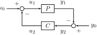
5. Robustness of Stability of Nonlinear Feedback Systems. The impor-tance of graph topology in the linear case is well known. In this section, we will show that it may also play a significant role in the nonlinear case by considering the system described by the configuration of Figure 5.1.
u0
u1 y1
P
C y0
u2 y2
−
+ +
[image:20.612.176.336.235.293.2]−
Fig. 5.1.Standard Feedback Configuration.
In this configuration, ui ∈ U, yi ∈ Y for i = 0,1,2, and both the plant P and
compensatorC are, in general, causal and nonlinear. We suppose all systems in this section are well-posed, that is, for each (u0, y0)⊤∈ Us× Ys, there exist unique signals u1, u2∈ U andy1, y2∈ Y such that
u0=u1+u2, y0=y1+y2, y1=P u1, u2=Cy2.
and the feedback operator
HP,C :Ws→ W × W :
u0 y0 7→ u1 y1 , u2 y2
is causal. Here,Ws=Us×Ys,W=U ×Y. The feedback stability of this system is the
requirement thatHP,Cis stable in a suitable sense. We are concerning the robustness
problem: when isHPλ,C stable given thatHP,C is stable andPλis a perturbation to
P?
In [7], this problem has been studied using a gap metric. Particularly, in the case where the linear gain is considered, it is proved that if HP,C is gain stable and Pλ
is close enough to P in the sense of gap metric, then HPλ,C is gain stable. Similar results are also given whenHP,C is (gf)-stable with super-linear growth. However in
the (gf)-stability case, the notion of convergence was not made explicit as no topology was indicated. In this paper, we consider the robustness of (gf)-stability when the convergence of Pλ to P is in the sense of any of the two graph topologies defined in
the previous sections.
We suppose Λ is a topological space and for eachλ∈Λ,Pλis a perturbation to the
nominal plant P =Pλ0. DefineM= Graph(P),Mλ = Graph(Pλ),N = Graph(C),
ΠN//M=I−ΠM//N. It is known thatHP,C is (gf)-stable (resp. gain stable) if and
only if ΠM//N is (gf)-stable (resp. gain stable), see [7].
A signal operator F : U → Y is said to be causally extendable if, for each
u ∈ U, y = F u and each τ > 0, there exists uτ ∈ Dom(F) such that Tτ(u, y)⊤ = Tτ(uτ, yτ)⊤ with yτ = F uτ. Henceforth, we suppose that P, C and each Pλ are
causally extendable.
Lemma 5.1. SupposeΦis a surjective mapping from M toMλ, Then, for any z∈ Wsand any τ >0, there existsxτ ∈ Ws such that
Tτz=Tτxτ+Tτ(Φ−I)ΠM//NTτxτ and TτΠMλ//Nz=TτΦΠM//NTτxτ.
Proof. Let HPλ,Cz = (z1, z2) with z1 = (u1, Pλu1)
⊤, z
2 = (Cy2, y2)⊤ for some u1∈ U, y2∈ Y. Then z=z1+z2 and ΠMλ//Nz =z1. By the causal extendability, for each τ > 0, there exist zτ
1 ∈ Mλ, zτ2 ∈ N such that Tτz1 = Tτzτ1, Tτz2 =Tτz2τ.
Since Φ is surjective from M to Mλ, there exists z3τ ∈ M with Φz3τ = z1τ. Write xτ=z3τ+z2τ. Thenxτ∈ Ws and ΠM//Nxτ=z3τ,ΠN//Mxτ =z2τ. Hence
Tτz=Tτz1+Tτz2=Tτzτ1+Tτz2τ =TτΦz3τ+Tτz2τ
=TτΦΠM//Nxτ+TτΠN//Mxτ =TτΦΠM//NTτxτ+TτΠN//MTτxτ
=Tτ(Φ−I)ΠM//NTτxτ+Tτxτ
and
TτΠMλ//Nz=Tτz1=TτΦz
τ
3 =TτΦΠM//Nxτ =TτΦΠM//NTτxτ.
For our main results, we will always require that the nominal plant satisfies a
k-coercive condition as stated below, note that this assumption will be not imposed on the perturbed plantPλ.
Definition 5.2. A signal operator P : U → Y is said to be k-coercive, with k∈ K∞, ifP has a coprime factorisation (N, D)such that
k(D, N)⊤uk ≥k(kuk) for allu∈ Us; (5.1)
Notice thatP isk-coercive if and only if
kLwk ≤k−1(kwk), for allw∈Graph(P), (5.2)
where L is the associated operator of (N, D). Hence any operator P with coprime factors is γ(L)−1-coercive, where L is the associated operator of a coprime
factori-sation, since (5.2) always holds with k−1(r) = γ(L)(r). It is of interest to observe
that a linear operator with coprime factors is alwaysk-coercive withk(r) =cr, c >0. Also note that ifP has a normalized coprime factorisation, thenP is 1-coercive and, therefore,c-coercive for anyc >0.
Proposition 5.3. Suppose that the nominal plantP is k-coercive and λ7→Pλ
is continuous at λ0 under a weighted topology Tω with w ∈ K∞. Then, for each λ,
there exists a surjective mappingΦλ:M → Mλ such that
sup
r>0
γ(I−Φλ)(k(ω(r)))
r →0, asλ→λ0. (5.3)
Proof. LetN D−1be the coprime factorisation ofP =P
λ0 satisfying the coercive condition (5.1). From Corollary 3.11, it follows that Pλ has coprime factorisation NλDλ−1 such that
sup
r>0
γ((D−Dλ, N−Nλ)⊤)(ω(r))
r →0, as λ→λ0. (5.4)
For eachλ >0 and eachu∈ Us, let
Φλ((Du, N u)⊤) = ((Dλu, Nλu)⊤). (5.5)
Φλ is a well defined, causal and surjective mapping from M to Mλ since Φλw =
((Dλ, Nλ)⊤Lw) withLthe left inverse of (D, N)⊤.
Now letr >0,(Du, N u)⊤∈ M withu∈ U
sand k(Du, N u)⊤k ≤k(w(r)). From
(5.1), it follows thatkuk ≤w(r), which implies k((D−Dλ)u,(N−Nλ)u)⊤k ≤ sup
kvk≤w(r)
k((D−Dλ)v,(N−Nλ)v)⊤k.
Therefore
γ(I−Φλ)(k(w(r))) = sup
(Du,N u)⊤∈Dom(I−Φλ) k(Du,N u)⊤k≤k(w(r))
k((D−Dλ)u,(N−Nλ)u)⊤k
≤ sup
kvk≤w(r)
k((D−Dλ)v,(N−Nλ)v)⊤k
=γ((D−Dλ, N−Nλ)⊤)(w(r)). (5.6)
By (5.4), we see (5.3) holds.
Remark. From (5.3), we see that kI−Φλkk◦ω → 0 which implies ~δ(P, Pλ) →
0 under a new weighted function ω1 = k◦ω. However, we cannot show whether ~δ(Pλ, P)→0 unless eachPλ is alsok-coercive. Also notice here the l.a.c. assumption
was not imposed. So (5.3) does not impliesPλ→P underd4.
Similarly, for the pointwise continuity, we have
Proposition 5.4. Suppose that P isk-coercive andλ7→Pλ is continuous atλ0
under the pointwise topologyT. Then, the mapping Φλ:M → Mλ defined in (5.5)
is surjective and thatγ(I−Φλ)(r)→0 for eachr >0, asλ→λ0.
Henceforth, we define the map Φλ to be as in Proposition 5.3 or 5.4 and give
robustness results under each graph topology. The following results follow as conse-quences of Proposition 5.3 or 5.4 and the results of [7]; however, we give the entire proofs for completeness. First, we consider the case when weighted topology is in-volved.
Theorem 5.5. Suppose P isk-coercive andHP,C is (gf)-stable. Ifλ7→Pλ is
then, for any n >0, there exists a neighbourhood Vn of λ0 such thatHPλ,C is (gf )-stable for λ∈Vn and
γ(ΠMλ//N)(r)≤γ(ΠM//N)
n+ 1
n r
+ 1
nr.
Proof. Letτ > 0, r >0 andz∈ W be given withkzkτ ≤r. By Proposition 5.3,
for each λ, there exists a surjective mapping Φλ :M → Mλ satisfying (5.3). From
Lemma 5.1, it follows that for eachλ, there existsxτ
λ∈ Ws such that Tτxτλ=Tτz−Tτ(Φλ−I)ΠM//NTτxτλ, TτΠMλ//Nz=TτΦλΠM//NTτx
τ
λ. (5.8)
By (5.3) and the properties ofγ, there exists a neighbourhoodVn ofλ0 such that γ(Φλ−I)(γ(ΠM//N)(kxτλkτ))
kxτ λkτ
≤ γ(Φλ−I)(k(w(kx
τ λkτ)))
kxτ λkτ
< 1 n+ 1
for alln >0 andλ∈Vn. So, from (5.8), it follows that
kxτ
λkτ≤ kzkτ+k(Φλ−I)ΠM//NTτxτλkτ
≤ kzkτ+γ(Φλ−I)(γ(ΠM//N)(kxτλkτ)))≤ kzkτ+
1
n+ 1kx
τ λkτ,
which implieskxτλkτ≤(n+ 1)kzkτ/n≤(n+ 1)r/nfor allλ∈Vn. By (5.8), we have TτΠMλ//Nz=TτΦλΠM//NTτx
τ
λ=TτΠM//NTτxτλ+Tτ(Φλ−I)ΠM//NTτxτλ
and therefore
kΠMλ//Nzkτ≤ kΠM//NTτx
τ
λkτ+k(Φλ−I)ΠM//NTτxτλkτ
≤γ(ΠM//N)
n+ 1
n r
+ 1
n+ 1kxλkτ≤γ(ΠM//N)
n+ 1
n r
+ 1
nr.
Sinceτ is arbitrary,γ(ΠMλ//N)(r)≤γ(ΠM//N)
n+1 n r
r+1
nr <∞forλ∈V0.
We remark that condition (5.7) can be replaced by the weaker condition:
γ(ΠM//N)(r)≤k(cw(r)) withc >0
sinceP is alsokc-coercive due to the remark made after Definition 5.2. This claim is also supported by Theorem 3.12 from which we see thatλ7→Pλis also continuous
at λ0 under a weighted topologyTcω, so the ω in (5.7) can be replaced by cω. This
replacement gives a weaker bound forγ(ΠM//N)(r).
In the case of the pointwise topology, we have:
Theorem 5.6. Suppose that P isk-coercive,HP,C is (gf)-stable andλ7→Pλ is
continuous atλ0under the pointwise topologyT. If, for eachλ,Tτ(Φλ−I)ΠM//N is
continuous and compact as a mapping from any subsetSr={w∈ W: supτ >0kwkτ ≤ r} toW, then for each r >0, there exists a neighbourhood Vr of λ0 in Λ such that γ(HPλ,C)(r)<∞for allλ∈Vr. Here Φλ is defined as in (5.5).
Proof. Letr >0 andw∈ W be given with kwkτ≤r. Consider the operator
SinceHP,C is stable,γ(ΠM//N)(k)<∞for allk >0. Using Proposition 5.3, we see
there exists a neighbourhoodVrofλ0 such that
k(Φλ−I)ΠM//Nxkτ ≤γ(Φλ−I) γ(ΠM//N)(2r)
< r (5.9) for all x∈S2r and λ∈Vr. This implieskAλxkτ <kwkτ +r < 2r for all x∈ S2r.
Due to our assumption, we may suppose thatAλ is continuous and compact on S2r.
From Schauder’s fixed point theorem, it follows that there existsxλ∈S2rsuch that xλ=w+ (Φλ−I)ΠM//Nxn forλ∈Vr,
ie.
w= ΠN//Mxλ+ ΦλΠM//Nxλ.
Since ΠN//Mxλ ∈ N,ΦλΠM//Nxλ ∈ Mλ and the perturbed system is well-posed,
we have
ΠMλ//Nw= ΦλΠM//Nxλ= ΠM//Nxλ+ (Φλ−I)ΠM//Nxλ and therefore
kΠMλ//Nwkτ=kΠM//Nxλkτ+k(Φλ−I)ΠM//Nxλkτ
≤γ(ΠM//N)(2r) +γ(Φλ−I) γ(ΠM//N)(2r)≤γ(ΠM//N)(2r) +r.
Henceγ(ΠMλ//N)(r)≤γ(ΠM//N)(2r) +r <∞forλ∈Vr.
With the technical assumption of compactness of Tτ(Φλ−I)ΠM//N, this result
states the boundedness ofHPλ,C(u0, y0)
⊤ fork(u
0, y0)⊤k ≤randλsufficiently close
toλ0. Obviously, if the neighbourhoodVr for (5.9) is independent ofr, that is, if γ(Φλ−I) γ(ΠM//N)(2r)< r, for allλsufficiently close toλ0
hold for all (large)r, thenHPλ,C would be (gf)-stable.
6. Conclusions. The main contributions of this paper are as follows. Natural generalisations of the graph topology w.r.t. to a gain function notion of stability for nonlinear systems in a general normed signal space setting were defined. Convergence in the graph topology was shown to have a natural application in robust stability results. Various metrizations of the graph topologies were given; in particular it was shown that the generalisations of the gap metric given by [7] and the natural generalisation of the graph metric both induce the graph topology when the stability notion is that of an (unweighted) induced gain, subject to certain assumptions on local asymptotic completeness and the existence of normalized coprime factorisations. Weaker results have been derived for the more general cases (including the weighted case). Georgiou-type formulas [4] have been derived and are shown to be equivalent to other alternative formulations of the gap metric.
Acknowledgements. The second author would like to acknowledge the hospi-tality of M.C. Smith and the Cambridge University Engineering Department for a visit during which this paper was completed. Informative discussions with M.C. Smith are gratefully acknowledged. The authors also thank the referees for valuable suggestions concerning the definition of normalized co-prime factorisations and the presentation of the paper.
REFERENCES
[1] B. D. O. Anderson, T.S. Brinsmead and F. D. Bruyne, The Vinnicombe metric for nonlinear operators,IEEE Tran. Auto. control,47(2002), 1450–1465
[2] B. D. O. Anderson, M. R. James and D. J. N. Limebeer, Robust stabilization of nonlinear systems via normalized coprime factor representations,Automatica,34(1998), 1593–1599 [3] M. Cantoni and G. Vinnicombe, Linear feedback systems and the graph topology,IEEE
Trans. Auto. Control,47(2002), 710–719
[4] T. T. Georgiou , On the computation of the gap metric,Systems&Control Letters,11(1988), 253–257
[5] T. T. Georgiou and M. C. Smith, Optimal robustness in the gap metric,IEEE Trans. Auto. Control,35(1990), 673-686
[6] T. T. Georgiou and M. C. Smith , Graphs, Causality, and Stabilizability: Linear, Shift Invariant Systems onL2[0,∞),Math. Control Signals Systems,6(1993), 195–223
[7] T. T. Georgiou and M. C. Smith, Robustness analysis of nonlinear feedback systems: an input-output approach,IEEE Trans. Auto. Control,42(1997), 1200–1221
[8] K. Glover and D. McFarlane, Robust stabilization of normalized coprime factor plant descrip-tions withH∞-bounded uncertainty,IEEE Trans. Auto. Control,34(1989), 811–830 [9] J. Hammer, Fractional representations of nonlinear systems: a simplified approach,Int. J.
Control, 46(1987), 455-472
[10] M. R. James, M. C. Smith and G. Vinnicombe, Gap metrics, representations and nonlinear robust stability, preprint.
[11] J. B. Moore and L. Irlicht , Coprime factorisation over a class of nonlinear systems,Int. J. Robust Nonl. Control, 2(1992), 261-290
[12] A. D. B. Paice and A.J. van der Schaft, The class of stabilizing nonlinear plant controller pairs,IEEE Trans. Auto. Control,41(1996), 634–645
[13] A.J. van der Schaft, Robust stabilization of a nonlinear systems via stable kernel represen-tations withL2gain bounded uncertainly,System&Control Letters,24(1995), 75–81
[14] A.J. van der Schaft,L2-Gain and Passivity Techniques in Nonlinear Control, 2nd edition,
Springer Verlag, 2002.
[15] J. M. A. Scherpen and A. J. Van der Schaft, Normalized coprime factorizations and balancing for unstable nonlinear systems,Int. J. Control,60(1994), 1193–1222
[16] J. A. Sefton and R. J. Ober, On the gap metric and coprime factor perturbations, Automat-ica,29(1993), 723–734
[17] E. D. Sontag , Smooth stabilization implies coprime factorisation,IEEE Trans. Auto. Con-trol,34(1989), 435–443
[18] M. S. Verma, Coprime fractional representations and stability of nonlinear feedback systems,
Int. J. Control, 48(1988), 897-918
[19] M. S. Verma and L. R. Hunt, Right coprime fractorizations and stabilization for nonlinear systems,IEEE Trans. Auto. Control,38(1993), 222-231
[20] M. Vidyasagar,Control System Synthesis, MIT Press, Cambridge, 1985
[21] G. Vinnicombe,Uncertainty and Feedback: H∞-shaping Control System Synthesis, Imperial College Press, 2001
[22] G. Vinnicombe, Aν-gap distance for uncertain and nonlinear systems,Proceedings of 38th IEEE CDC, Phoeniz, AZ, (Dec. 1999), 2557-2562