Geographically intelligent disclosure control for flexible aggregation of census data

AGGREGATION OF CENSUS DATA

C

Y

,

D

M

,

C

S

A

This paper describes a geographically intelligent approach to disclosure control for protecting flexibly aggregated census data. Increased analytical power has stimulated user demand for more detailed information for smaller geographical areas and customized boundaries. Consequently it is vital that improved methods of statistical disclosure control are developed to protect against the increased disclosure risk. Traditionally methods of statistical disclosure control have been aspatial in nature. Here we present a geographically intelligent approach that takes into account the spatial distribution of risk. We describe empirical work illustrating how the flexibility of this new method, called local density swapping, is an improved alternative to random record swapping in terms of risk-utility.

Geographically intelligent disclosure control for flexible

aggregation of census data

CAROLINE YOUNG, DAVID MARTIN, CHRIS SKINNER

ABSTRACT

This paper describes a geographically intelligent approach to disclosure control for protecting flexibly aggregated census data. Increased analytical power has stimulated user demand for more detailed information for smaller geographical areas and customized boundaries. Consequently it is vital that improved methods of statistical disclosure control are developed to protect against the increased disclosure risk. Traditionally methods of statistical disclosure control have been aspatial in nature. Here we present a geographically intelligent approach that takes into account the spatial distribution of risk. We describe empirical work illustrating how the flexibility of this new method, called local density swapping, is an improved alternative to random record swapping in terms of risk-utility.

Keywords: privacy, census data, spatial analysis, small area geography, quality issues

GEOGRAPHICALLY INTELLIGENT DISCLOSURE

CONTROL FOR FLEXIBLE AGGREGATION OF

CENSUS DATA

CAROLINE YOUNG

(corresponding author: [email protected])

School of Social Sciences, University of Southampton, Highfield, Southampton, SO17 1BJ

DAVID MARTIN

School of Geography, University of Southampton, Highfield, Southampton, SO17 1BJ

CHRIS SKINNER

1. Introduction

Small area population data from censuses provide an important base layer in many GIS

applications. Indeed, census geography played a key role in early GIS data structure

development (Peucker and Chrisman, 1975). The ability to produce such detailed data is

due to censuses’ unique combination of detailed information about individuals and

households with coverage of an entire population. However, achieving a complete or near

complete response rate also makes the data highly susceptible to disclosure. Disclosure occurs when an individual can be identified in the data, leading to potentially sensitive

information being revealed (Lambert, 1993). Protecting the confidentiality of census data

by application of statistical disclosure control (SDC) methods is an integral part of the census process allowing use of protected data by researchers and policy makers across all

sectors. SDC methods either restrict or modify the detail released (Willenborg and de Waal,

2001). Internationally, government statistical organizations undertake population data

collection under various legislative frameworks (Holt 2003) which generally embody strict

confidentiality requirements. The importance of the issue is magnified by reliance of

official statistics on public trust in the safeguards employed. Historically, disclosure

control could be handled by checking outputs manually before publication. However, in the

past two decades, increases in computing power have stimulated increased demand on the

part of census users, who are able to employ complex analytical techniques and process

larger amounts of data. The growth of digital geographical information allows for the

possibility of automatically generating census geographies as required (Openshaw and Rao

sufficient to meet users’ demands. Many researchers require data which does not fit into

neat aggregations of published zones. In the UK, for example, changes in health service

organization creates demand for census data which cannot be matched by reaggregation of

standard outputs. Such demand pressures have led to discussion of the development of

flexible tabulation systems in, for example, the UK, Australia and the US (Rhind et al.

1991, Zayatz 2003, Duke-Williams and Rees, 1997). Any such system would allow users to

create their own customised tables from unpublished individual records. In the absence of

such systems, there is ongoing pressure for the production of outputs for multiple small

area geography systems.

The disclosure risk facing statistical organizations is two-fold: first, the risk from outputs

for any small population and, second, the additional risk from publishing multiple

overlapping aggregations. There is particular demand for tables of counts at

neighbourhood level but these are potentially risky since it may be possible to recognise

data relating to particular individuals, especially in the light of local knowledge.

Identification of individuals may lead to potentially sensitive information being revealed.

The difficulty of multiple outputs is that published tables, although independently safe, may

be compared with one another in order to reveal new information. This is particularly a

problem when data are published for multiple geographical boundaries, described by

Duke-Williams and Rees (1998) as geographical differencing. The response of the UK statistical

organizations has been to publish counts only for hierarchical aggregations of the smallest

output areas.

A closely related disclosure issue, arising from the availability of geographically

disaggregate level. While not usually considered in the context of aggregate census data,

there is a close link to the central focus of this paper. Leitner and Curtis (2006) draw a

distinction between statistical (attribute) and spatial (locational) confidentiality. Statistical

confidentiality is associated with individual information, in GIS terms the equivalent of

aspatial attributes, while spatial or locational confidentiality is concerned with the

placement of individual-level statistical information on a map. To date, relatively little has

been written about methods to protect the point mapping of individual information although

this is of increasing concern to the GIS community. Geoprivacy is especially sensitive in

studies of health and crime data.For example, law-enforcement agencies throughout the US

provide crime maps (Leitner and Curtis, 2006), while point maps are often published

representing cases of cancer or infectious diseases (for example, Zimmerman and Pavlik

2006, Armstrong et al. 1999). Leitner and Curtis (2006) note that an individual’s

residential location can be easily displayed, potentially leading to identification of the

individual and disclosure of confidential information as inverse address matching

technology can be used to reveal the street address and residents at a point location

(Zimmerman and Pavlik, 2006).

The conventional approach to preserving spatial confidentiality in these data has been to

adopt the same methodology as for census data, that is to aggregate records across

populations large enough to ensure prevention of disclosure (Armstrong et al. 1999).

However, aggregation damages the data, making research into causation with associated

factors very difficult (Leitner and Curtis, 2006). Armstrong et al. (1999) introduced the

term geographical masking (geomasking) for the modification of geographical coordinates

Affine transformations relocate each point by change of scale, rotation, flipping or some

concatenation of these masks. Random perturbation or jittering involves adding noise to original locations. According to Armstrong et al. (1999), random perturbation is an

effective geomasking technique, to some extent superior to affine and aggregation masks.

Kwan et al (2004) have assessed the spatial masks discussed in Armstrong et al. (1999),

particularly levels of random perturbation in relationship to disclosure risk since mapped

locations of disease or crime contain wide variation in of population density. The amount of

noise added to location can be allowed to vary with population density.This idea has also

been discussed by VanWey et al. (2005) who simulated a sampling frame of public schools

in the US. Their data contained the geographical location of each school with potentially

sensitive attribute information. A solution was proposed whereby map symbol size was

adjusted to cover multiple schools, providing locational uncertainty in proportion to a

specified level of identification risk. For schools in large cities (densely populated) a much

smaller point buffer was needed than in remote rural areas.

In this paper we propose a geographically intelligent method of statistical disclosure

control for aggregate census data which draws on elements of these geoprivacy approaches

by protecting the locations of individual records. Although described in the census context,

the method would be applicable to administrative or survey data. In the following section

we review the disclosure control problem. In section 3 we consider traditional record

swapping methods which are essentially aspatial and propose a local density swapping

approach which takes into account the distribution of population as a spatial indicator of the

risk of disclosure. Furthermore, we examine ways of offering greater protection against

The remainder of the paper then considers an empirical application of the record swapping

approaches. Section 4 describes the creation of a census-like microdataset; section 5

presents some measures of risk and utility and section 6 presents the results of our analysis.

The results of our experiments are discussed in section 7 before drawing conclusions

identifying further research priorities.

2 Statistical Disclosure Control

2.1 Census Tables

We here outline the production of aggregate census data, drawing specifically on UK

practice but with international applicability. A census collects data on attributes (e.g. age

or household size) for individuals and households. The objective is usually to collect data

from the entire population, although in reality some will be missed. For the purposes of

this discussion we will disregard the many practical challenges of enumeration which in

various ways affect data quality and consider the creation of data for publication from the

database of census responses.

Tables of counts are produced by cross-classification of subsets of attribute variables.

Counts will typically be for either individuals or households and, for generality, we use the

term unit to denote the individual, household or other set of individuals upon which the

counts are based. Geographical coordinates ( , )X Y are associated with each unit, typically

by matching to a master address list. The data available for tabulation are compiled into a

microdata file, represented by anN×(K+2) matrix, Z, where N is the total number of

as well as values of ( , )X Y for the different units. We refer to the N units as the population.

Tables for publication are formed by specifying output zones and attribute categories and

counting the number of units that fall into each unique combination of output zone and

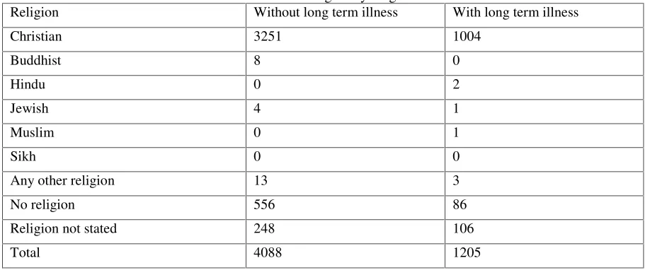
category. For example, Table 1 provides a fictitious illustration of a cross-classification of

religion by long term illness (both variables in the 2001 census in the United Kingdom) for

5293 individuals in a given zone. Such tables represent spatial aggregations of the

microdata file.

Table 1: Fictitious Census table: Religion by long term illness for Zone H Religion Without long term illness With long term illness

Christian 3251 1004

Buddhist 8 0

Hindu 0 2

Jewish 4 1

Muslim 0 1

Sikh 0 0

Any other religion 13 3

No religion 556 86

Religion not stated 248 106

Total 4088 1205

2.2 The Disclosure Problem

We are concerned with the disclosure risk which may arise from the publication of multiple

frequency tables of the type described in the previous section. There are various ways of

defining disclosure for tabular outputs (Willenborg and de Waal, 2001). Most

commentators suppose the existence of an intruder who has access to the published tables

basic notion is that of identity disclosure or identification, which arises if it is possible for

the intruder to establish a one-to-one correspondence between an element of a table and a

known unit in the population (Bethlehem et al., 1990). Such a possibility is of particular

concern to census agencies, as it would contradict the confidentiality undertakings made to

respondents. For illustration, Table 1 reveals that in output zone H there is only one

Muslim. If, via another source of information, the intruder knows the name and address of a

Muslim who lives in zone H then they can establish a correspondence between this

individual and an element in the table. Thus, identity disclosure would have taken place.

Identity disclosure may occur more readily for cells with counts of one, termed cell

uniques, and we treat these as risky.

It might be argued that such identity disclosure is not serious since the intruder does not

gain any new information about the respondent. However, identity disclosure can be

associated with attribute disclosure, which arises if the intruder can learn additional information about a unit from the published output. For example, the intruder who knows a

Muslim living in zone H can learn from Table 1 that this individual suffers from a limiting

long term illness. Identity disclosure is not, however, a necessary condition for attribute

disclosure. For example, an intruder who knows someone in output zone H whose religion

is Hindu can learn that they must have a long term illness, despite there being two such

people and thus identification has not taken place. Despite such considerations, we shall in

this paper focus on the risk arising from identity disclosure. Focusing on cell uniques also

gives us an overall indicator of disclosure risk (since the more ones there are, the more

Tables produced for non-coterminous geographies may be independently safe, but when

published together, can sometimes be subtracted or differenced to reveal sensitive

information relating to a geographical ‘sliver’. This has been termed the geographical

differencing problem (Duke-Williams and Rees, 1998) and occurs when one or more output

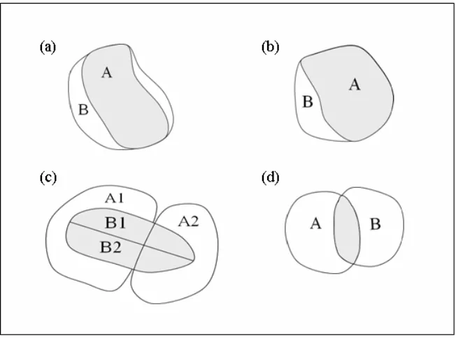
zones nest entirely within another as in Figure 1.

Figure 1: Geographical Differencing Problem: Output zones which nest within one another

Suppose Table 2 relates to output zone B in diagram (a) or (b) in Figure 1 and Table 3

relates to output zone A, then subtracting the corresponding cells (Table 3 from Table 2)

reveals a new Table 4 which relates to the differenced zone. All the non-zero cell counts

are cell uniques. The geographical differencing scenario can be extended to consider output

zones which when aggregated can, in combination, be differenced from a larger aggregate:

for example, in diagram Figure 1(c), B2 + B1 can be differenced from A1 + A2. Sections of

no way of knowing which data units in the two tables belong to the intersecting area, as in

Figure 1(d). These examples demonstrate the problems of publishing tables relating for

multiple systems of output zones. Small slivers can result producing many small cell counts

which are potentially disclosive. This can occur through both nested and non-nested

geographies. Providing user access to an interactive tabulation tool would present many

differencing problems.

Table 2: Illustrating the Geographical Differencing Problem - Fictitious Table representing Geography A

16-20 21-30 31-40 …

Benefit claimed 10 16 19 …

Benefit not claimed 8 12 11 …

Table 3: Illustrating the Geographical Differencing Problem - Fictitious Table representing Geography B

16-20 21-30 31-40 …

Benefit claimed 9 16 19 …

Benefit not claimed 8 11 11 …

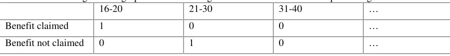
Table 4: Illustrating the Geographical Differencing Problem - Fictitious Table representing Differenced Area

16-20 21-30 31-40 …

Benefit claimed 1 0 0 …

Benefit not claimed 0 1 0 …

2.3 Statistical Disclosure Control (SDC) Methods for Tabular Outputs

A variety of SDC methods have been proposed to protect against the kinds of disclosure

risk described in the previous section. They may be divided into pre-tabular methods,

which are applied to microdata before aggregation into tables, for example by modifying

the values of the attribute variables and post-tabular methods, which are applied to the tables, for example by rounding all cell counts to multiples of some base number, such as

zone-independent, assuming that they only involve modification of the microdata file, Z (see

section 2.1) and that standard spatial aggregation is used to form the tables from the

modified microdata. If the base microdata are ‘safe’ then any aggregation must also be safe.

Pre-tabular methods are generally more flexible, with parameters that can be varied to

achieve a balance between disclosure risk and utility. Utility refers to the quality of the

output after SDC and can be assessed by analyzing the impact of SDC methods on

statistical analysis (Shlomo, 2006). Pre-tabular methods can cause statistical damage to the

resulting tables that is difficult for the users of these tables to measure. Hence, the

parameters of these methods are often set in a way to minimize this damaging effect

(Shlomo, 2005). Post-tabular methods are zone-dependent since they must be applied

afresh to every new table that is produced for a given output zone. Not only must any risk

assessment be updated for each tabulation, but it is in theory necessary to assess that the

new table cannot be combined with previously released tables to undo the protection that

was previously applied. Post-tabular methods can be cumbersome to apply, particularly for

very large tables. Current solutions involving rounding techniques (Salazar et al, 2004) are

still in development for very large tables with a complex hierarchy of subtotals to ensure

that marginal totals add up correctly whilst maintaining a high quality table. The fact that

the pre-tabular SDC methods only need to be applied once is an important advantage

compared to post-tabular methods, when the aim is to produce tables for multiple

geographies. The remainder of this paper focuses on pre-tabular methods. In reality, the

choice between these approaches is not straightforward and a combination of pre- and

development of a method which balances risk and utility, avoiding the need for further

post-tabular adjustment.

3 The Proposed SDC Approach

Pre-tabular methods of SDC could involve modification of either attribute variables or

geographical coordinates. The former has the major disadvantage that it can result in the

introduction of inconsistencies between the attribute variables, such as a married

10-year-old. This type of anomaly will not occur as a result of modification of the geographical

coordinates since most census attributes will be consistent with any geographical location.

We therefore consider here only geographical perturbation methods, defined as those SDC

methods which modify the true spatial locations of some or all of the units in the microdata.

Thus, the coordinates (Xi,Yi) of a unit i are modified to new coordinates

(

)

refer to the distance between the old and new locations as the perturbation distance. Usually

the perturbation distance, d is measured in Euclidean space:

(

) (

)

i i i

i X Y Y

X

d = − + − ₍₁₎

Geographical perturbation methods may be expected to reduce disclosure risk in the

aggregated table since it will not be known whether an observed cell unique in a table

corresponds to a unit which genuinely falls in that cell or indeed whether the true cell count

is one. Geographical perturbation could be implemented in a number of ways. One

approach, applied in the geoprivacy literature to point data is that of displacement, where

procedure (Armstrong et al., 1999). One problem with this approach is that it cannot be

guaranteed that the displaced locations will be feasible, for example they might fall in a

self-evidently unpopulated area such as a lake. An alternative which overcomes this

problem and avoids the need for detailed validation of new locations is record swapping,

where pairs of units are selected from the population and the coordinates of each pair are

swapped while the global set of locations is unchanged. We will focus on record swapping

approaches, firstly considering in section 3.1 an established method which has been

employed in practice by several census agencies (Shlomo, 2005 and Zayatz, 2006). Our

proposed new approach is introduced in section 3.2.

3.1 Random Record Swapping (RRS)

Random record swapping (RRS) is a pre-tabular method of geographical perturbation

resulting in the geographical variables of two units i and j being swapped. Thus, the

geographical coordinates (X_i,Y_i) are exchanged with( , )X Y_{j j} but the attribute variables

remain unchanged. Different approaches may be adopted for deciding which pairs of units

are swapped. Often, pairs of units are matched in some way to limit the potential damage to

resulting analyses. Following Willenborg and de Waal (2001), the ith record of the

microdata may be partitioned into three sub-vectors: Mi, Ai*and (Xi,Yi), where Miis a

vector of match variables, defining a subset of the attribute variables to be controlled when

seeking recipient households for swapping, and *

i

A is a vector containing the remaining

attribute variables. Thus, only records j with Mj =Mi are considered for swapping with

Three features of RRS can be modified, each of which may affect both disclosure risk and

utility. First, the smaller the fraction of records selected for swapping, the lower both the

expected risk reduction and distortion. Second, the more variables and categories which are

used to match pairs of values the less distortion, but this may lead to difficulties in finding

matching records for all recipients. Third, swapping can be targeted on records deemed

most ‘risky’, determined by prior analysis of the small counts in tables (Zayatz, 2006). The

UK 2001 censuses were disclosure-protected by RRS in combination with a post-tabular

SDC method (Shlomo, 2006). The 2000 US census employed targeted swapping (Zayatz,

2003) in combination with post-tabular methods. The specific details of record swapping,

such as the proportion of records swapped, are kept confidential so as not to aid an intruder.

To illustrate RRS further, we present the basic approach adopted in England and Wales in

2001. The units swapped were households. Match variables consisted of a hard-to-count

index1, household size, and a broad age and sex distribution of individuals within the

household (Shlomo, 2005). A sample of households was swapped between Output Areas

(OAs: small area building brick for release of 2001 census data) within Local Authority

Districts (LADs: larger area containing around 50,000 people) (Boyd and Vickers, 1999),

that is each record in the sample was paired with a matching record from a different OA

within the same LAD. Thus, LAD is effectively a match variable also and this method is

zone-dependent, being based on specific LADs and OAs. A key drawback of such RRS is

that membership of the same LAD is the only control over the distance and direction of

perturbation, which may result in significant damage to statistical analyses involving spatial

elements finer than LADs.

3.2 Local Density Swapping (LDS)

The proposed local density swapping (LDS) method is designed to overcome this key

drawback, by applying pre-tabular perturbation to the microdata in a way which is not

dependent upon the choice of output zones. The first feature of the method is that

perturbation distances are sampled from a probability distribution. This allows greater

control because the type of distribution can be selected, as can its parameters such as mean

and standard deviation.

The risk of identifying an individual by differencing depends on the proximity of other

individuals with similar characteristics. For example, an elderly man located in an area with

mainly young people will present a high disclosure risk. In general, the more people there

are in the area, the more likely it is that someone else will share the same characteristics –

following Tobler’s first law of geography (Tobler, 1970) similar characteristics are most

likely to be found together. Thus a fundamental predictor of disclosure risk is population

density. In a densely populated urban area, less perturbation is generally needed to disguise

the true location of a household. A similar concept was identified earlier in the geoprivacy

literature (Armstrong et al. 1999, VanWey et al, 2005), masking locations of disease or

crime on a map in proportion to population density. Density is not taken into account by

conventional approaches to record swapping. Thus in a densely populated region, more

perturbation than necessary may be added to a household. Our second key proposal is to

as opposed to Euclidean distance. The household distance n is a measure of the number of households between swapped households.

Our third proposal aims to reduce the risk from geographical differencing by swapping

more records but by smaller distances. Thus a cell unique in a differenced area should have

a likelihood of having been perturbed. Perturbation at the local level will minimise damage

but introduce uncertainty. In practice this could be implemented by swapping broadly at the

same scale as the small area geography (for the UK this might be adjacent postcodes for

example, or blocks in the US) with variation depending on population density. Postcodes or

blocks represent local areas for which an intruder might know detailed information about

their neighbours and around which we might want to add noise. The initial sample of

records selected for swapping could be random within strata (as in the random record swap)

to ensure even protection against risk.

One advantage of LDS is its flexibility. Statistical organizations differ in their assessment

of tolerable levels of risk and utility. LDS parameters can be varied to achieve an

appropriate balance between risk and utility. Parameters that can be varied include the

sampling fraction, the probability distribution, the sample size and selection and match

variables. Very rare records with unusual combinations of characteristics (such as a 16

year-old-widow) are unlikely to be protected by swapping (as they tend to be unique

irrespective of geography) but these are likely to require separate recoding or suppression

4 Creating a Test Dataset

It is not possible to use an actual census database due to the census confidentiality

constraints. However, anonymised microdata samples and small area aggregations are

available from the UK censuses (Dale and Teague 2002, Dale and Marsh, 1993). In this

section we briefly describe the creation of a synthetic microdataset created from these

sources to create a 100% dataset consisting of the full set of census variables, to which we

assign point locations. The aim is to create a dataset that is realistic for testing disclosure

control methodologies rather than to accurately replicate a specific regional population.

4.1 Synthetic Population

Our synthetic population is based on 1991 UK census microdata, as 2001 files were not

released until after the commencement of this work. We use the Household Sample of

Anonymised Records (SAR), a microdata file for a 1% sample of individuals in

households, including the complete set of census variables but with geographical coding

limited to Standard Region. We also use Small Area Statistics (SAS), which give

information on individuals and households in tabular form at enumeration district (ED)

level, the smallest areas in the 1991 census geography. EDs are similar in size to OAs

containing around 200 households or 450 people. SAS tables contain the entire population

for each small area. However the table dimension is small, containing only two or three

variables, so the joint distribution for the full set of census variables is not known.

Microsimulation techniques are used to estimate this joint distribution at the small area

individuals drawn from the microdata sample, broadly preserving actual marginal

characteristics.

Since swapping involves distorting the relationships between geography and attribute

data, it is important to study an area which is spatially heterogeneous. The county of

Hampshire in Southern England was chosen because of its diverse characteristics. It

includes two densely populated urban areas (Portsmouth and Southampton) and extensive

rural areas. The population of approximately 1.5 million displays wide variety of economic

activity, household structure and individual characteristics. The county comprises 3175

EDs in thirteen LADs with population densities ranging from 138 people per km2 _in

Winchester to over 4000 people per km2 in Portsmouth.

A microdataset with a realistic spatial distribution is needed in order to investigate the

effects of locational swapping. There are various techniques available including iterative

proportional fitting based on a set of small area tables (Williamson et al., 1998) or synthetic

probabilistic reconstruction (Birkin and Clarke, 1989), but here we use a method of

combinatorial optimisation developed by Williamson and Voas (2000). This approach uses

the SAR as the parent population from which households can be drawn to recreate

populations for individual EDs. This is performed iteratively by selecting a combination of

households from the SAR that best reproduces the characteristics of the ED. Constraints on

the combination of households chosen are provided by known tabulations of ED data from

the SAS. We have chosen four small area tables from the 1991 small area statistics

covering age, marital status and sex; household space type and tenure of households;

household. The more tables used as constraints, the more iterations are required to give a

good level of fit.

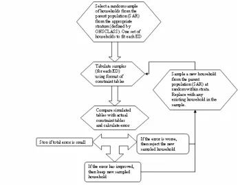
Figure 2 gives an overview of the microsimulation process. The first step is selection of

an initial sample of households for each ED. Rather than sampling at random, the

ONSCLASS variable (Wallace et al, 1995) was used to stratify the SAR records.

ONSCLASS is a census-based classification of wards present on both the SAR and SAS.

This is a very useful variable since it provides a key to the characteristics of the ward in

which the household is located. An initial sample was taken at random from the stratum

representing the same ONSCLASS as the ED. Communal establishments were excluded

from our analysis. At each iteration a new household is sampled from the appropriate

stratum and if the fit is improved the new household kept, otherwise it is dropped. This

iterative process continues until a satisfactory fit is achieved. To measure fit we compared

the simulated table frequencies, denoted F_c, to the constraint table frequencies, denoted

c

O , (Ballas et al. 1999, Williamson and Voas, 2000). The subscript c denotes a cell in the

table for which the constraint frequencies are available. We used a measure called Total Absolute Error less than 3, denoted TAE and defined by:

TAE =

∑

This fit measure ignores absolute errors |Oc−Fc| of less than 3 in order to speed up the

Figure 2: An overview of the microsimulation process

The resulting synthetic population provided an adequate fit to the published tables using

this approach. There were no clusters of error which may have raised concerns that an area

with unusual characteristics had not been fitted properly. Urban areas showed the worst fit

but overall the TAE was relatively small at approximately 2 to 4 individuals or households

per cell. 70% of households were not unique, with 15% of households sampled three times

(representing 45% altogether) but less than 1% represented more than four times. This

would be a problem if the objective involved assessing uniques in the entire microdataset

since only 30% are unique records. However there are many uniques at the small area level

in tables of two to four variables. Moreover the majority of repeated households are located

in different LADs. This is an important consideration because households could be

better on the synthetic population than on a real population). An additional consideration is

that both the LDS and RRS tests will be equally affected by any biases in the synthetic

population.

4.2 Creating Spatial Locations

Creating spatial locations for the households is particularly important because these will be

used by the swapping procedure. There are no files directly recording household locations

in the UK. Instead, the directory of postcodes and enumeration districts was used, which

provides a household count for each ED-postcode intersection and grid references for each

postcode (Martin, 1992). Unique locations were created for households by adding noise

around postcode locations, proportional to ED population density. An incomplete sort of

households by tenure type was performed before grid reference allocation, resulting in

households of similar tenure displaying some spatial clustering.

Figure 3: Creating artificial household locations

The smallest postcodes do not have formally defined boundaries, so these were generated

postcodes identified, using the deldir2 package in the statistical package R. We thus create

a synthetic micropopulation for Hampshire consisting of individuals within households

having a full set of census variables. Each household has a unique point location and is

assigned to a postcode, ED and ward. The postcodes have synthetic boundaries but do not

necessarily nest entirely within EDs; EDs nest entirely within wards and wards within

LADs.

5 Implementing and Evaluating the Swapping Methodology with the Test Dataset

This section describes the implementation of the general methodology proposed in Section

3 using the statistical program SAS and the synthetic population and presents measures for

the assessment of risk and utility. We refer to the synthetic data as the ‘original’

(unswapped) data.

5.1 Swapping Methodology

RRS and LDS are performed by selecting an initial sample of households from the

population and then finding matching households with which these will be swapped

(section 3). Match variables of ethnic group, family type, number of persons in household

and tenure are used. These were chosen as being similar to those used in the actual 2001

UK census RRS. RRS requires matching households in a different ED but within the same

LAD.

To implement LDS, a ‘distance’, n, is generated randomly from an exponential

distribution with a specified mean λ for each of the households in the initial sample. This

distance will determine the number of households, n, in the circle for which the initial

household is at the centre and the matching household is on the circumference. For ease of

computation, households are assigned to a 100m raster and a cellular approximation to a

circular search performed. The circular band corresponding to number of households n, is

then determined by counting the households in successive bands until the cumulative count

is greater or equal to n. The outer band of households contains the nth household.

Generating n from an exponential distribution ensures n cannot be negative and has a rapidly decreasing probability of taking a large value. The probability density function of n

is given by:

( )

f n _=λ− −e λ _{, n≥0 (3)}

so thatλ =E n( ). In the following experiments a value of λ has been specified which

represents an average distance between adjacent postcodes. A random swap of 10% of

households between adjacent postcodes was performed and λ was determined as the mean

number of households between all pairs of swapped households. The minimum and

maximum from this 10% random postcode swap was also used to truncate the distribution

to prevent swapping over very long distances or very small distances.

Once the circular band containing the nth household is determined, a best matching household from the households in this band can be found using the match variables of

ethnic group, tenure, persons in household, family type. Households which have previously

been swapped are penalized and discouraged from swapping a second time.

Following Duncan et al (2001), we propose to evaluate the effectiveness of the swapping

methods in a risk-utility framework, i.e. we study the performance of each of the methods

in terms of both disclosure risk and the utility of the resulting outputs for analysis.

Moreover, since the methods depend upon the specification of parameters, such as the

proportion of records to swap, we shall study how such choices affect risk and utility and

the trade-off between the two. In order to set up this framework we need to introduce

measures of risk and utility.

5.2.1 An Indicator of Disclosure Risk Disclosure protection can be measured by

comparing disclosure risk before and after perturbation. In section 2, we discussed how risk

before perturbation could be measured in terms of cell uniques. A crude measure would be

the number of cell uniques. After perturbation, cell uniques may also be considered, since

these might be a natural target for an intruder, but it would be inappropriate to still measure

risk by the number of cell uniques, since these may no longer be genuine. Instead, the

probability that an observed cell unique (after perturbation) represents an actual unique is

considered.

Such measures of risk are clearly dependent upon output zones. These may be EDs or

wards, for example. To measure the risk arising from geographical differencing, the

disclosure risk for frequency tables for zones assumed to be equivalent in scale to a

differenced ‘sliver’ is considered, for which the smallest zones available are postcodes (and

are independent of the geographies used in the methodology).

The cells in a table T are defined by cross classifying a subset of the attribute variables in

the categories of this subset of attribute variables. Let Fc denote the cell frequency in a

specified zone, that is the number of units in the zone with the specified combination of

values of the attribute variables. To be explicit about the effect of the perturbation process,

let o c

F denote the cell frequency before perturbation and p c

F the cell frequency after

perturbation. Also let nT denote the number of cells in table T and let match = 1 if

1

o p

c c

F =F = and if the same unique household appears in the table before and after

perturbation. A cell count of one after perturbation is called a true unique if match = 1, i.e.

if it was also a count of one in the original table and it relates to the same household. The

probability of finding a true unique is thus:

)

Pr(TU = ( 1& 1)

( 1)

T

T

n o p

c c

n p

c

I F F match

I F

= = =

=

∑

∑

where the sums are over all the cells c in the table and I is an indicator function which equal 1 if true, 0 otherwise.

5.2.2 Measures of Utility Utility will be measured in terms of distortion to the data, i.e.

in terms of dis-utility. Specifically, we measure the absolute average deviation per cell

(AAD) averaged across all tables at a particular level of geography. AAD will be measured

on tables formed by cross-classifying age, sex and marital status. These variables were

chosen as they contain vital demographic information which should not be distorted and

since they do not include any of the matching variables. The measure is defined as:

AAD =

T

n p o

Section 6.5 considers some additional measures of utility, which assess how swapping

distorts spatial features of the tables.

6 Results of Applying Swapping Methodology to Test Dataset

6.1 Comparison of 10% RRS with 10% LDS

We begin our analysis by simulating a 10% RRS, taken to be a realistic option which might

be employed in a census, and compare with a 10% LDS. The methods are applied to the

entire synthetic population of Hampshire. The same initial 5% random sample (forming one

half of the swapped records) was used in both cases, with the number of records selected

proportional to the total population in each ward. This ensured an even distribution of

records for swapping over the entire county.

Table 5 presents disclosure risk in terms of (a) percentage of ‘true uniques’ and (b)

number of true uniques per 1000 population at risk. We assess disclosure risk in tables of

long term illness and ethnicity since these variables are likely to produce many small cell

counts. Table 5(a) shows that using matching variables (the variables Mi (section 3.1) on

which both households must match for a swap) as opposed to swapping households at

random, the resulting disclosure risk is higher. There is very little difference between the

two methods when swapping only 10% of households. More importantly the disclosure risk

after applying both RRS and LDS is very high at all levels of geography at over 80%. This

means there is a high probability that a cell count of one relates to the original household.

This is likely to be considered unacceptable by a statistical agency and in this case it would

seem sensible to apply a post-tabular method to the data (as in 2001). Table 5(b) also shows

true uniques per 1000 population at risk. At higher levels of geography, there are far fewer

uniques.

Table 5: Assessing Disclosure Risk (Percentage of True Uniques) (a) DISCLOSURE RISK (proportion of true uniques)

Postcode ED Ward

10% Random Record

Swap (with matching)

0.94 0.88 0.81

10% Random Record

Swap (without matching)

1.00 0.93 0.88

10% Local Density Swap

(with matching)

0.89 0.92 0.92

(b) DISCLOSURE RISK (number of true uniques per 1000 population at risk)

Postcode ED Ward

10% Random Record

Swap (with matching)

7.55 3.13 0.30

10% Local Density Swap

(with matching)

6.79 2.92 0.27

Table 6 presents the utility of the data after swapping, measured in terms of deviation

between cell counts in the original and protected tables. As before, an average is taken over

all tables at a particular level of geography. In general the LDS produces smaller average

cell deviations.

Table 6: Assessing Utility (Absolute Average Distance)

UTILITY Postcode ED Ward

10% Random Record Swap (non-matching)

10% Random Record Swap (matching)

0.25 0.17 1.11 1.09 6.66 5.75

6.2 Increasing the sampling fraction

Since the 10% swap results in high disclosure risk we next examine how the risk-utility

outcome changes as we increase the total proportion of records swapped. In this scenario,

we use only a sub-region of the synthetic population relating to the Basingstoke and Deane

local authority because the methods are computationally intensive. Initial samples are

drawn which when paired with matched households make total swapped samples of 10%,

25%, 50%, 70%, 90%, 100%. In this case the samples were completely random with no

stratification by ward. Moreover each sample was independent meaning that the 10% RRS

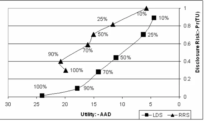
initial sample was different to the 10% LDS initial sample. In figure 4 we measure risk at

postcode level as it is the sliver level which presents the greatest disclosure risk (see table

5). The measure used is the probability of being a true unique. However, utility is measured

at ward level representing a more common scale for analytical use.

The graph shows how LDS improves upon RRS across all sampling fractions. Thus, for a

given utility (a vertical line on the graph), LDS always has a lower disclosure risk at

postcode level than RRS. Conversely, for a given level of risk (a horizontal line on the

graph), LDS always achieves greater utility at ward level than RRS. Suppose a statistical

agency wanted to ensure disclosure risk was below 0.5; following figure 4, they would need

to swap approximately 70% of the records to achieve this through RRS but around 50% of

the records would need to be swapped if LDS was used. Moreover if 50% of records were

swapped with LDS, we would still obtain higher utility at ward level than if 70% of the

records were swapped with RRS.

6.3 Changing the Mean Perturbation Distance for LDS

The sampling fraction is one parameter of the LDS method that can be changed. Another is

the mean perturbation distance. This distance is measured in terms of number of households

and thus doubling the perturbation distance does not mean the households are moved twice

as far in Euclidean space. The relationship between the area of the circular band and the

radius of the circle containing n households is not linear and this needs to be taken into account when selecting an appropriate perturbation distance. A small sample size of 10%

would require setting λ≥10,000 households to reduce disclosure risk by a significant

amount (less than 50%) with an average distortion of 5 per cell. On the other hand, with a

sampling fraction of 70%, to reduce disclosure risk below 0.5 at ward level, λ = 2,000

6.4 The relationship between Geography and the R-U Outcome

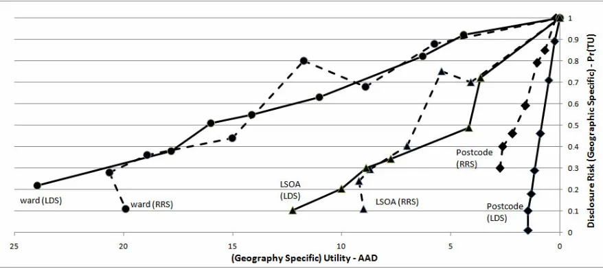
In Figure 5, we show the general pattern in terms of risk-utility over different output scales.

These results include a completely independent geography derived from the 2001 census:

Lower Super Output Areas. LSOAs are larger than EDs but smaller than wards. Risk here

is measured in terms of the probability of being a true unique for the respective geography

(i.e. postcode, LSOA or ward). Utility is the AAD for the respective geography. The figure

shows a definite scale effect. As the zone size increases, the utility worsens in terms of

AAD, with wards having the greatest average cell deviation and postcodes having the

smallest average cell deviation: the larger zones of course have larger populations.

However, the most important effect observable in Figure 5 concerns the disclosure risk at

postcode level. LDS results in better utility (lower AAD) and lower risk than RRS for

equivalent sampling fractions (0%, 10%, 25%, 50%, 70%, 90%, 100%) as indicated by the

positioning of the lines. However, it is difficult to detect any difference between the

methods at the higher levels of geography; partly because of the more unpredictable effect

of RRS. Similar patterns were picked up for OAs and EDs (not much difference between

Figure 5: Comparing the Risk-Utility Outcome of LDS with RRS over different levels of geography

The sample sizes have been omitted from the graph for clarity; however the lines are joined

in order of increasing sample size.

6.5 Spatial Measures of Utility

Measurement of utility in terms of AAD may have masked underlying effects not picked up

by averaging. In this section we attempt to study utility in more depth. As discussed in

section 3.1, the perturbation methods swap a record i with values

(

)

i i i

M A X Y with a

record jwith values

(

)

j j j

M A X Y so that, after swapping, record i has

values

(

)

i j j

M A X Y . Thus, the relationship between the match variables M and the

attribute variables _A* _{is unchanged. Similarly the relationship between the geography and}

match variables is unchanged. For example, we would expect the relationship between

tenure and occupation to be the same after swapping. In fact this is an important advantage

example, distorts the interrelationships between the attribute variables, often artificially

increasing correlations (Shlomo, 2005; 2006). However, the relationship between the

geography variables and the attribute variables is distorted with swapping. Thus when

searching for appropriate utility measures, it would seem sensible to focus on measures in a

spatial context. In this section we shall study utility primarily at LSOA level, representing a

common scale for policy-making and analysis.

6.5.1 Changes in spatial rank We first consider how zones change relative to one another

in terms of their ranking for a particular attribute. We are interested in changes in overall

spatial pattern, such as would alter the shading classes on a choropleth map; that is changes

in rank order rather than changes in scale. We here sort zones according to an attribute and

assign these ranks into groups, comparing the rank group for each zone before and after

swapping.

The test will be carried out on LSOAs for two different attributes: (1) percentage

unemployment and (2) percentage of male head of households, aged 35-50, in a

professional job with a first degree or higher. As with any large mixed urban/rural area,

these attributes are likely to vary over space. The latter is a category formed from a

cross-classification of the variables and will show the extent to which interactions of the variables

are distorted by geography. The LSOAs are split into deciles. We present the results in

Table 7 as absolute percentage change (in rank group) showing the median of the

approximate normal distribution and the maximum. The table shows that, in general, LDS

results in fewer rank changes than RRS. The cross-classified attribute histograms also

showed similar patterns so have not been included here. This indicates that the underlying

Table 7: Absolute Percent Changes in Rank Group for LSOAs: Comparing LDS and RRS for 25% and 80% swaps.

RRS25 LDS25 RRS80 LDS80

Median 2 1 2 2

Maximum 7 9 9 20

Proportion no

change

29/103 36/103 11/103 17/103

6.5.2 Effect on Spatial Autocorrelation Another way of assessing changes in spatial

distributions is to study the effect on clustering / spatial autocorrelation (Fotheringham et

al, 2002). Swapping is likely to distort patterns of spatial autocorrelation. In particular,

swapping over large distances is likely to make the data more homogeneous and pockets of

households exhibiting unusual characteristics would tend to become more like the region as

a whole. Therefore if we know of a variable (or set of variables) which exhibit spatial

dependency, we can exploit this relationship to assess the effect of the two swapping

methods.

Typically a single measure of spatial autocorrelation is calculated which describes an

overall degree of spatial dependency across the whole dataset. Local measures of spatial

autocorrelation allow spatial variations in the spatial arrangement of data to be examined

(since a global measure may mask the true pattern). In this section we will assess spatial

autocorrelation for the two attributes (a) percentage unemployed and (b) percentage of male

head of households aged 35-50 in a professional job with a first degree. The results for the

swapped populations will be compared against the original data.

(

)

(

)

(

)

,

( )

u v u v

u v

u v u

u v u

m w Z Z Z Z

I

w Z Z

− −

=

−

∑ ∑

∑ ∑

∑

where mis the number of zones

u

Z is the percentage in a particular category of a variable or a cross-classification of

variables A, for zone u

Zis the mean of the percentages across all zones

uv

w is an element of a contiguity matrix, taking the value 1 if zone uis a neighbour of zone

v _{and 0 otherwise.}

Values of Moran’ s I larger than 0 indicate positive spatial autocorrelation; values smaller

than 0 indicate negative spatial autocorrelation.

Spatial autocorrelation at a local level will be measured using the LISA statistic (Local

Indicators of Spatial Association) computed as:

(

)(

)

(

)

uv u v

v u

u u

w Z Z Z Z

I Z Z − − = −

∑

∑

Maps can be produced showing the value of I_ufor each zone u. In the LISA maps,

high-high and low-low relate to incidences of positive spatial autocorrelation whereas high-high-low

and low-high relate to incidences of negative spatial autocorrelation. The Moran’ s I and the

LISA maps were computed in GeoDa3 and relate to the Basingstoke and Deane local

authority.

3 _{GeoDa is a spatial analysis software tool developed at the Spatial Analysis Lab, University of Illinois;}

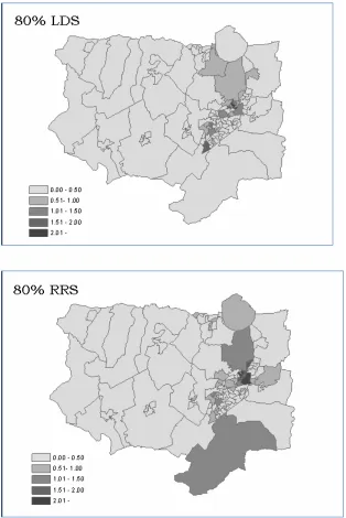
6.5.2.1 Spatial Autocorrelation for Percentage Unemployed The LISA maps in Figure 6

were computed for LSOAs in Basingstoke and Deane comparing the absolute change in Iu

between the original unswapped data and the swapped populations (for samples of 25% and

80%). The original LISA map (not pictured here) showed evidence of negative spatial

autocorrelation north of the centre of Basingstoke but positive spatial autocorrelation in

central and southern Basingstoke. The nearest neighbour weights matrix was used with

eight nearest neighbours selected. This means that there is some randomness in which

‘neighbours’ are selected (if there are more than eight nearest neighbours). For this reason,

the same weights matrix was used in every case. Figure 6 shows that at the 80% level, there

are significant amounts of absolute change in I_uparticularly in and around the central urban

area. There is more change for RRS than LDS as indicated by the darker shadings of the

LSOAs with absolute change being greater than one in several LSOAs. At the 25% level

there were only small changes for both RRS and LDS (not displayed in this paper). All

swapped populations were found to have fewer significant areas of spatial autocorrelation

as the sampling fraction increases suggesting that the data, after swapping, is possibly

Figure 6: LISA maps showing Absolute Change in I_i between the original (unswapped) data and the

swapped data, for LSOAs for %unemployed.

0.3491 for the original data and changes very little at 25% swapping. At 80% it fell to

0.2341 for RRS while remaining at 0.3338 for LDS.

6.5.2.2. Spatial autocorrelation for Percentage in a Category of a Cross-Classification

We now turn to the percentage in a category of a cross-classification of variables,

represented by the percentage of male head of households, aged 35-50, with a first degree

or higher in a professional job. As expected this percentage is broadly inversely related to

levels of unemployment. As before, most of the structure is retained at the 25% swap rate,

perhaps more so for the LDS, with little change in I_u for the LSOAs (not shown). On the

other hand at the 80% level, there is major damage to the autocorrelation structure as

indicated by the dark shaded LSOAs for RRS in Figure 7. Further investigation for RRS

showed that many of the significant LSOAs showed incorrect directions of spatial

autocorrelation after swapping. This observation is also supported by Moran’ s I. At 25%

the spatial correlation is little changed from the 0.2640 for the original data for both RRS

and LDS. At 80% swapping this has reduced to 0.0367 for RRS whereas for LDS it

remains at 0.2336. RRS swaps over much larger distances, having the potential for much

greater damage than LDS swapping, primarily over shorter distances. This divergence

Figure 7: LISA maps showing Absolute Change in I_i between the original (unswapped) data and the

swapped data, for LSOAs for % male heads in professional job aged 35-50 first degree.

OA-level maps (not shown) display similar patterns to the LSOA maps shown here but the

the work in this section provides some evidence the LDS is less damaging to the detailed

spatial data structure than RRS.

6.6 Discussion of Results

We here discuss some of the principal themes emerging from our results. Swapping records

shorter distances and in proportion to local population density using the LDS method does

seem to be effective in reducing disclosure risk at the postcode level and has the important

benefit that it permits small area tables to be produced with less risk and provides stronger

protection against geographical differencing. Although more noise is added at the local

level, similar levels of protection and damage to those seen for more conventional methods

are observed for larger zones. In addition, LDS makes no reference to pre-existing

geographical boundaries and is thus more resilient to future reaggregation and differencing

challenges.

We have begun to assess the utility of the new method by studying the changes in spatial

relationships after swapping. The LISA maps showed that with LDS, the most significant

patterns in the data still remained after a large proportion of records were swapped.

However with RRS, patterns were lost at lower levels swapping, particularly for the

cross-classified attribute. Changes in rank order indicated that LDS was altering the data less than

RRS, which is particularly relevant to GIS and mapping applications. LDS achieved a

better outcome than RRS at the postcode level, producing smaller average cell deviations in

a table made up of the independent variables age, marital status and sex. Many different

utility measures could be employed but in general LDS retains higher utility than RRS

households in high density areas being moved only short distances. In general, this

contributes to the RRS results being more unpredictable than those for LDS.

A statistical organization would normally desire that disclosure risk should be less than

50% so that the odds are against an intruder finding a true unique. Ideally the disclosure

risk would be even smaller than this, at around 10% or less. Swapping a 10% sample under

either method was very ineffective and the percentage of true uniques remained above 80%.

Even swapping 25% of the data resulted in a disclosure risk still above 50% at all levels of

geography and this helps to explain why utility remained so high in the LISA maps at this

level. Also at the 25% swap level, the order of rankings was not disturbed too greatly. To

reduce the disclosure risk below 10% for all levels of geography would probably mean

swapping around 90-100% of the records under either method. Organizations would

probably consider it unacceptable to implement such high swapping levels, which means it

is unlikely that swapping could ever be used as a sole protection method and would

probably always have to be combined with some post-tabular modification.

7 Conclusion

Statistical agencies wishing to provide outputs by flexible geographies need to protect

against the geographical differencing problem which may arise. Pre-tabular disclosure

control methods are most attractive for this purpose, because they need only be applied

once, ensuring that any tables and resulting differenced areas must also be safe. In this

paper, we have proposed the LDS method as an alternative to the established RRS method

and have argued that it may provide greater protection at the local level as well as allowing

employs greater spatial intelligence and whether or not record swapping alone is judged to

provide sufficient protection, it is a powerful disclosure control method which may provide

a more efficient balance of risk and utility particularly for GIS applications. A census user

might only know the percentage of records swapped but this still affords a large degree of

uncertainty around each cell. This contrasts with post-tabular methods such as rounding

where an intruder can usually deduce a narrow uncertainty interval around each cell in

relation to the rounding base. Moreover local swapping is a good way of providing

confidentiality protection whilst ensuring the plausibility of the data. RRS often moves

households out of their local area and thus if the two areas are very different (moved from

an inner city zone to a rural zone for example), it could be obvious that a household has

been swapped presenting both a disclosure risk and reduction in accuracy of the data. More

work needs to done to study other measures of disclosure risk and utility. Risk assessment

may, for example, be extended by looking at disclosure from zeros and other small cells

and not just from cell uniques. Another idea might be to obtain two similar geographies and

analyse the differencing risk attributable to the two swapping methods.

With regard to utility, most GIS use of census-type data currently ignores the impacts of

disclosure control methods whereas these may in fact significantly affect geographical

analysis results. Measurement of utility is far from straightforward. AAD, used here, is

limited because it is an absolute value, not relative to the original cell values and since it is

an average, it can mask underlying detailed effects. However AAD has provided a useful

initial evaluation of the effects of changing the parameter values for swapping, due to its

ease of calculation. It is important to remember that the work in this paper has been carried

unique characteristics of this dataset. Since LDS is dependent on population density, it

would be a logical extension to study the effects in regions of high and low density more

closely. Moreover, we have focused here on record swapping, but it would also be possible

to perform other types of geographical perturbation such as displacement using standard

GIS functions which are being used for geoprivacy purposes. A more comprehensive

examination of utility after swapping would need to more carefully address the spatial

operations that GIS census users typically apply. Much more work needs to be done, both

to fully understand current practice and with regard to future census data production.

Acknowledgements

This work was funded by an ESRC postgraduate studentship: PTA-042-2004-00013.

SAR and SAS census data were taken from the Census of Population Programme web

pages funded by the ESRC and additionally JISC: http://www.census.ac.uk/default.htm

References

ARMSTRONG,M.P.,RUSHTON,G., andZIMMERMAN,D.L., 1999, Geographically masking

health data to preserve confidentiality. Statistics in Medicine, 18, 497—525

BALLAS,D., CLARKE,G. and TURTON,I., 1999, Exploring microsimulation methodologies

for the estimation of household attributes.In 4th International Conference on