Flow and likely scour around three dimensional seabed structures evaluated using RANS CFD

(1)

Flow and likely scour around three dimensional seabed structures evaluated using RANS CFD

By

Guillaume de Hauteclocque,

Justin Dix, David Lambkin, Stephen Turnock

University of Southampton

Ship science Report No:144

(2)

Chapter: Summary

2 Summary

When a structure is placed on the seabed, tidal or other marine current induce areas of flow acceleration and deceleration. This may result in movement of the seabed substrate (often sand) near the structure. It would be useful to be able to assess possible scour. For example when considering the protection of wreck and other marine sites of archaeological interest, or the long term durability of marine renewable and offshore structures mounted on the seabed.

The first step in the process of scour calculation is to get a good description of the flow around the structure; next a scour pattern can be estimated. The work which was carried out can be divided in 4 mains parts of increasing complexity. The first objective was to produce and compare results on the well documented case of a surface mounted cube. Next, the conclusions of this first part were use to perform several calculations around a variety of cuboids, the CFD results were compared with experimental data obtained recently by the NOC. The third part was a study of scour around a modeled wreck, using experimental data from a recent thesis. Finally, full scale measurements of the “unknown wreck” were used to complete the study.

(3)

Chapter: Summary

3

4

5.1 Geometry ... 51

5.2 Mesh and calculation setup. ... 52

5.3 Results ... 53

5.3.1 Comparison with the cuboids 5:1... 53

5.3.2 Roughness effect ... 54

5.3.3 Wall shear value and threshold of motion. ... 55

5.3.4 Scour onset estimation from CFD result. ... 56

5.3.4.1 Case 1 ... 56

5.3.4.2 Case 2 ... 60

6- Full scale comparison ... 65

6.1 Configuration ... 65

6.2 Whole half flood tide averaging ... 68

6.2.1 Input data ... 68

6.2.2 Results ... 70

6.3 Middle flood tide average ... 72

6.4 Early flood tide average ... 76

6.5 Late flood tide average ... 81

(5)

Chapter: List of Figures

5 List of Figures

Figure 1 : Very coarse mesh (5000 elements) ... 18

Figure 2 : First results, not realistic ... 19

Figure 3 : Mesh ... 19

Figure 4 : vector plot in the symmetry plane ... 20

Figure 5 : 3D view ... 20

Figure 6 : y+_{plot ... 21}

Figure 7 : Blocking (O-grid around the square) ... 22

Figure 8 : Distribution of the nodes on the radial edge ... 22

Figure 9 : 2D mesh ... 23

Figure 10 : Streamlines around the square cylinder ... 23

Figure 11 : "Vortex Street” k-ε calculation, velocity colour plot and streamlines. ... 24

Figure 12 : mean velocity streamlines ... 25

Figure 13 : Flow around a surface mounted cube according to [11]... 26

Figure 14 : Grid 3 bottom view ... 28

Figure 15 : Comparison of side force a) LES b) SST c) SAS-SST ... 30

Figure 16 : symmetry-plane streamline. ... 31

Figure 17 : Wall shear stress obtain with the different turbulence models ... 33

Figure 18 : velocity profile at X/D = 2.5 and X/D=4 ... 34

Figure 19 : turbulence kinetic energy at x/D=1 and x/D=2 ... 35

Figure 20 : Horseshoes vortex visualisation. Isosurface of the mean second velocity gradient invariant. Q=0.01 s^-2 ... 37

Figure 21 : The arc-shaped vortex behind the cube is visualized by plotting the isosurface P=-0.56 Pa. ... 38

Figure 22 : Instantaneous isosurface Q=0.009 s-2 LES, SAS and SST ... 39

Figure 23 : Average and maximum wall shear stress ... 39

Figure 24 velocity shape compared to the experiment and visualisation of the horseshoes vortex. Ratio 2:1, AoA=67,5 °, Re=80 000 ... 44

(6)

6

Figure 26 : k-ε (Left) and SST (right) Aspect ratio 5:1, AoA 45 °, Re=80 000 ... 46

Figure 27 : Streamlines SST above and k-ε below, the results are very similar Aspect ratio 5:1, AoA 45 °, Re=80 000 ... 46

Figure 28 k-ε (Left) and SST (right) Ratio 3:1, AoA=22,5 °, Re=80 000 ... 47

Figure 29 : TKE/TKE input ... 48

Figure 30: Input velocity profiles, for δ/H=0.5 and δ/H=5 ... 49

Figure 31: Dimensionless wall shear stress ... 50

Figure 32 : Vessel geometry... 51

Figure 33 : mesh ... 53

Figure 34 : visualisation of the vortex structures. Q isosurface. 45 deg ... 54

Figure 35 : Wall shear ... 54

Figure 36 : general view of the flow ... 57

Figure 37 : wall shear stress ... 57

Figure 38 : Turbulent kinetic energy just above the seabed. ... 58

Figure 39 :Wall shear stress, immobile sand in deep blue. Threshold of motion reached everywhere else. ... 58

Figure 40 : Scour prediction ... 59

Figure 41 : 225 experimental scour patterns... 59

Figure 42 : Coupled model principle ... 60

Figure 43 : Wall shear stress ... 60

Figure 44 : Velocity just above the seabed ... 61

Figure 45 : turbulence kinetic energy just above the seabed ... 61

Figure 46 : Streamline ... 62

Figure 47 : Wall shear stress ... 62

Figure 48 : Experimental scour pattern ... 63

Figure 49 : superimposition scour and TKE. ... 63

Figure 50 : unknown wreck site location ... 65

Figure 51 : Scour on the full scale wreck compared to the turbulence kinetic energy around a cuboid ... 66

Figure 52 : unknown wreck site ... 66

Figure 53 : Flow measurement (from [18]) ... 67

(7)

7

Figure 55 : Mean direction measured by the probe 1 during a half flood tide. ... 68

Figure 56 : Mean velocity profile, probe 1 ... 69

Figure 57 : probe 6 direction and velocity profile. Averaging during the whole half flood tide ... 70

Figure 58 : probe 8 direction velocity profile Averaging during the whole half flood tide ... 70

Figure 59 : probe 9 direction velocity profile Averaging during the whole half flood tide ... 71

Figure 60 : Flow direction evolution during the flood tide ... 72

Figure 61 : streamlines around the wreck a) from the probes b) from the inlet (2.8m) c) from the inlet (3.5m) ... 73

Figure 62 : Probe 6 profiles Middle flood tide ... 74

Figure 63 : Probe 8 profiles Middle flood tide ... 74

Figure 64 : probe 9 profiles Middle flood tide ... 75

Figure 65 : Turbulence kinetic energy, Depth, Wall shear and velocity plots a)TKE b)depth c)wall shear stress d)velocity ... 76

Figure 66 : probe 6 profiles early flood tide ... 77

Figure 67 : Probe 8 profiles ... 77

Figure 68 : Probe 9 profiles ... 78

Figure 69: Turbulence kinetic energy, Depth, Wall shear and velocity plots a)TKE b)depth c)wall shear stress d)velocity ... 79

Figure 70 Bottom: middle flood tide / Top: early flood tide Right: velocity / Left: TKE (Same colour scale) ... 80

Figure 71 : probe 6 Late flood tide ... 81

Figure 72 : Probe 8 Late flood tide ... 82

Figure 73: Probe 9 Late flood tide ... 82

(8)

Chapter: List of Tables

8 List of Tables

Table 1 : Summary of the square case calculation ... 25

Table 2 Meshes, number of nodes ... 27

(9)

Chapter: List of Tables

9

Nomenclature

Cd : drag coefficient Cl : Lift coefficient f : frequency

h : Heigth of the cuboid

k or TKE: turbulent kinetic energy

Re : Reynolds number based on the height of the structure St : Strouhal number

u : Velocity U : Mean velocity u’ : Fluctuating velocity

y+_{: Normalised distance in direction normal to wall}

δ : Boundary layer thickness

μ : dynamic viscosity

μt: eddy dynamic viscosity

ρ : density (kg/m3)

ε : Turbulence dissipation rate : Body force term

Xr: Reattachment length

Xs: Upstream separation length

Acknowledgements

(10)

Chapter: Introduction

10 Introduction

Context, aims and objectives

When a structure is placed on the seabed, tidal or other marine current induce areas of flow acceleration and deceleration. This may result in movement of the seabed substrate (often sand) near the structure. It would be useful to be able to assess possible scour. For example when considering the protection of wreck and other marine sites of archaeological interest, or the long term durability of marine renewable and offshore structures mounted on the seabed.

The first step in the process of scour calculation is to get a good description of the flow around the structure. In this work, the structures of interest are three dimensional (3D), (i.e. with a finite (small) height relative to length/breadth). The aim is to investigate a reliable and cost-effective (from a computational point of view) way of calculating the flow around representative 3D surface-mounted structures. In particular, to examine the quality of prediction of the wall (seabed) shear stress, which is the main parameter of interest for scour initiation.

Previous work in the area

(11)

Chapter: Introduction

11

It is, however, harder to find results on other shape likes cuboids with other aspect ratio or angle of attacks. The results from [9] provide experimental data which will be reproduced by CFD calculation in this study.

When considering calculations to examine scour around structures, the data available involves very often an infinite cylinder, either mounted vertically or horizontally, (Horizontal for submarine pipelines and vertical for many anchoring systems). Experimental results from Saunder’s thesis are available [16], this thesis gives results for scour around a model scale wreck in a water channel (flume).

Layout of the work

(12)

Chapter: Computational tools

12 1-

Computational tools

1.1 Governing equation

1.1.1 Reynolds-Averaged-Navier-Stokes

The behaviour of a fluid is defined by the Navier-Stokes equations, which for an incompressible Newtonian fluid can be written as:

Continuity equation:

Eq 1

Momentum equation:

·

Eq 2

(13)

13

, Eq 3

, Eq 4

The unsteady Reynolds-Averaged-Navier-Stokes equations are obtained combining the Eq 1, Eq 2, Eq 3 and Eq 4:

0

Eq 5

· · · , , Eq 6

1.1.2 Turbulence modelling

The Reynolds-averaging of the complete Navier-Stokes equations raises 6 additional

unknown variables:

·

, , those terms are called “Reynolds stresses”. Turbulence

(14)

14

• RANS Two-equation models

The basis for almost all two-equation models is the Boussinesq Eddy-viscosity assumption [17]. This assumption is that the Reynolds stress tensor is proportional to the mean strain rate tensor. This can be written as

·

, ,

2

Eq 7

is the eddy viscosity which has to be computed and k is the turbulence kinetic

energy : , ,

The two-equation models bring two extra transport equations to represent the turbulent properties of the flow. The turbulence is assumed to be isotropic (which is not true for most flows)

The k-ε model defines an equation for the turbulent kinetic energy k, and another one for the dissipation rate ε. The eddy viscosity is eventually defined by the Eq 8.

Eq 8

This model is the most used in the industry; it however has difficulties to describe satisfactory results for separated flow. [4]

(15)

15

The SST (shear strain rate) model has been developed to combine the assets of the k-ε and k-ω model. The k-ω model is used near the wall and the k-ε model used in the free-stream zone. Thus, the advantages of the k-ω model, including an efficient near wall treatment, are conserved, but the main drawback is corrected by using the k-ε model. A blending function is used to ensure a smooth transition between the two formulations. [7]

• RANS Reynolds Stress model SSG

The Reynolds Stress Models do not include the Boussinesq assumption; the Reynolds stresses components are directly computed

A Reynolds Stress Model includes transport equations for the individual components of the Reynolds stress tensor and the dissipation rate (i.e. 6 equations). This formulation takes into account the turbulence anisotropy. This turbulence approach includes more equations than the previous turbulence model and thus requires a larger computational time. In spite of the more complete physical description, the results are not always better than with a two-equation turbulence model.

• SAS-SST

(16)

16

1.1.3 LES formulation

The LES formulation can be considered to be halfway between RANS and DNS, indeed, with an LES calculation the equations are filtered; the largest scales of the turbulence are resolved exactly without any modelling. The fine time and space scales have then to be resolved by a subgrid-scale model. With Ansys CFX, the Smagorinsky model is available. This formulation requires a very fine mesh and a very fine time step. Reliable statistics on the turbulence require moreover a large number of time steps. This method is thus computationally expensive and will not be studied extensively.

1.2 RANS Solver details

The RANS solver used in this work was CFX 11, a fully implicit finite volume code. The advection scheme used was “high resolution”, with this setting the blend factor (between first and second order scheme) varies throughout the domain. The scheme is thus both accurate and bounded. For more detail about this scheme see [3]. For transient calculations, the transient scheme used is the “second order backward Euler”. The second order backward Euler scheme is an implicit time stepping scheme, second order accurate. However, this scheme is inappropriate for some quantities as turbulence or volume fraction (which must be bounded); the scheme used for the turbulence equation will therefore remain First Order.

As with most RANS solvers, CFX 11 use the residual from the continuity and momentum equations as a measure of convergence with a value of 5e-5 set for almost all of the calculations.

1.3 Grid generation

(17)

17

mesh will be structured or unstructured. For unstructured grids, the meshes will be composed of hexa elements, with several prism layers near the walls. An increased density will also be set in the wake of the structure.

Meshing step for structured grids:

1. Define the geometry

2. Divide the geometry in several blocs 3. Set the number of nodes on each edge

Meshing step for unstructured grids: 1. Define the geometry

2. Define the mesh size on each surface, define the “density area” 3. Generate the surface mesh

4. Smooth the surface mesh 5. Generate the volume mesh 6. Smooth the volume mesh 7. Generate the prism layers 8. Smooth the volume mesh

1.4 Computational resources

(18)

Chapter: Preliminary calculations

18 2-

Preliminary calculations

2.1 Initial study

As part of the process of applying the commercial code Ansys CFX version 11 [3], a few tests have been made. The geometries chosen were simple: 2D square or 3D mounted cube. Several kinds of mesh have been tested, the first ones, generated with CFX-Mesh, were very coarse (less than 70 000 cells,) to allowed fast calculations. The calculation domain size has been tested on those meshes. It appears that if the length downstream is to short, the outlet boundary condition has an effect on the flow. Figure 1 shows a view of the 2D mesh

The calculations are steady-state, (RANS with a K-epsilon turbulence model).

The meshes have been generated with CFX-mesh. This software is really easy to use; the integration with the modeller and the solver is efficient as well. Figure 1 shows a mesh generated by CFX-mesh.

Figure 1 : Very coarse mesh (5000 elements)

(19)

19

confirms the need to determine the mesh density and the distance needed upstream, downstream and above the structure.

Figure 2 : First results, not realistic

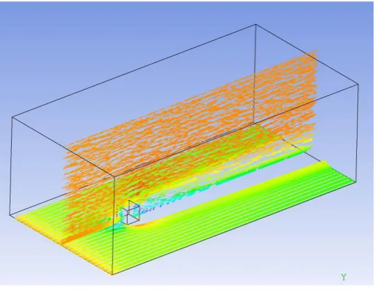
3D calculations have also been run. The mesh, which has been refined near the wall, is still coarse (less than 100 000 elements) but the calculation domain is long and high enough. Assuming that the flow would be steady state (this assumption is not right, see next section), the symmetry plan is used to reduce the calculation time. Figure 3 is a perspective view of the mesh; compared to the previous calculation, the domain size has been extended. Figure 4 presents a vector plot in the symmetry plane; the size of the domain is deemed big enough.

(20)

[image:20.595.164.436.277.487.2]

20

Figure 4 : vector plot in the symmetry plane

Figure 5 : 3D view

(21)

[image:21.595.158.444.56.289.2]

21

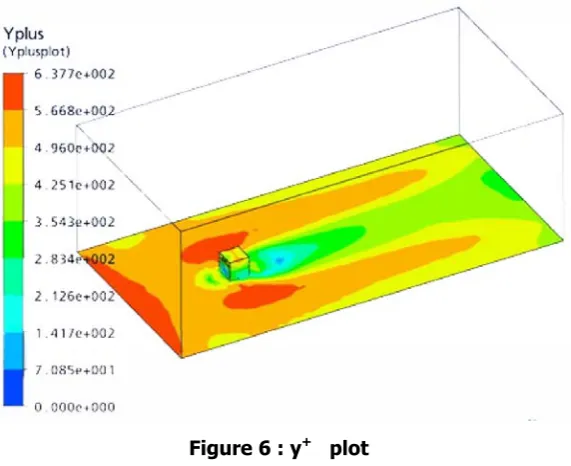
Figure 6 : y+_plot

The mesh is still too coarse near the walls therefore, the boundary layer is not well computed.

2.2 2D Calculation with finer meshes

2.2.1 Steady-state simulation

The following meshes were generated with ICEM, which allows far more mesh control than CFX-mesh. The mesh is structured; an O-grid is defined around the cylinder. The geometry is the one described in Rodi’s paper [1]; the domain is thus extended as follows around the 2D square (D is the height is the square):

• 4,5 D upstream • 15 D Downstream

(22)

[image:22.595.237.348.423.571.2]

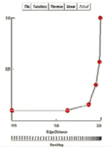
Chapte Figure is defin the squ The rad er: Prelimin 7 shows th ned around

uare cylind

dial mesh i

nary calcula he blocking d the squar

er. The fin

Figure

is set to be

Figure 8 : D

ations g strategy re, this aut nal grid is p

7 : Blockin

e very fine

Distribution

for the 2D tomatically presented i

g (O-grid a

near the s

n of the nod

D square c y means th

in Figure 9

around the s

square as s

des on the

cylinder: a hat the me 9.

square)

shown on

radial edge

an O-grid b esh is refin

Figure 8.

e

blocking ed near

(23)

Chapte On the slip. Th side siz Figure coloure The co calculat compar reattac er: Prelimin e top and o

he simulati ze).

10 present ed with the

omputed d tion quote red to ex chment len

nary calcula on the bot

on is done

ts the resu e velocity m

Figure 10

drag coeff ed in the R

xperimenta ngth (5.5)

ations

Figu

ttom, the b e with a Re

ult using st magnitude.

0 : Streamli

ficient is C Rodi’s pap al values

is over pre

ure 9 : 2D m

boundary c eynolds nu

reamlines .

ines around

Cd = 1.73 per [1]. Ho

of betwe edicted by

mesh

conditions umber of 2

starting fro

d the squar

3. This m owever, th een 1.9 a

more tha

are set to 2 000 (bas

om the inle

e cylinder

matches wi his value is

and 2.2. n 300%.

o a wall wi sed on the

et; they ar

(24)

24

not surprising, indeed the actual flow is unsteady and the present calculations provide a steady-state result, so the flow is unlikely to be well described this way.

2.2.2 Transient calculations: URANS, LES

[image:24.595.133.466.354.577.2]

The following test aims to reproduce the vortex shedding effect behind the square cylinder. The calculation is thus transient. The Reynolds number of the calculation is again set at 22000. As the result is expected to be unsteady, the symmetry line is not used. The unsteadiness appears by itself; an initial perturbation is not needed. Figure 11 plots the velocity contours and streamlines, the “vortex street” appears clearly.

Figure 11 : "Vortex Street” k-ε calculation, velocity colour plot and streamlines.

(25)

25

Figure 12 : mean velocity streamlines

• LES calculation

The LES calculation requires a 3D mesh; the depth of domain is then extended to 4D, the boundary conditions at the end of the cylinder remain symmetrical. The LES simulation provides a better estimation of the Strouhal number (which is experimentally very precise) and shows an irregular vortex shedding. To give a more precise (statistically significant) result, the LES calculation should be run for a much larger amount of time. The LES calculation need a 3D calculation and takes therefore more time to be performed.

Table 1 : Summary of the square case calculation

Size (nodes)

Turbulence Model

Time Step

CPU time

Total Time

St Cd Cd

rms

Cl rms

Ir

23 000 k-ε Steady

-state

- 1.7 0 0 5.5

23 000 k-ε transient 2.5s 5 h 8000s 0.15 1.92 0.023 0.74 1.5

110 000 LES 3D 2.5s 10 h 4000s 0.136 2.23 0.027 1.12 1.1

(26)

Chapter: Flow around a surface-mounted cube.

26 3-

Flow around a surface-mounted cube.

The aim of this section is to consider the different ways to assess the flow around a cube, Figure 13, examining the precision compared to experimental results and computational requirements, and to determine which approach is the most suited for the desired result quality. An ultimate calculation requiring a huge computational time is not looked for, thus the RANS model will be preferred, and the meshes tested will not be very fine (wall function would be required).

3.1 Geometry and meshes

(27)

27

Grid dependency and turbulence model tests are performed on the well documented case of a surface-mounted cube.

In spite of the simple geometry, the flow around a surface mounted cube at high Reynolds number is complex, massively separated and turbulent (thus often used as a benchmark test for the turbulence model). The flow first separates in front of the cube, leading to a horseshoe vortex. An arc vortex structure appears behind the cube.

The Reynolds number based on height is 40 000. The calculation domain size is extended as follows (H is the cube height):

• 5H upstream • 15 H downstream • 9H laterally

In order to match with the available results (Rodi [1]), the top wall is set with a no slip condition. The Y+_{value on the top surface does not allow the capture of the} boundary layer. The top boundary layer can be assumed independent from the rest of the flow. An additional calculation with refined mesh near the top wall has validated this assumption.

The post-processed values are the reattachment length and velocity profiles. As the purpose of this document is the seabed scour, the wall shear stress will be also investigated (in spite of the lack of available experimental results on this data).

The grids tested are presented in the Table 2

Table 2 Meshes, number of nodes

Grid (cube) 1 2 3 4

Number of nodes

(28)

28

For each of these grids, the mesh is structured, refined near the floor and around the cube (The structure of the mesh around the cube is an O-grid). Figure 14 shows a bottom view of the grid. These meshes have been generated with ICEM CFD 10. As the flow might show unsymmetrical unsteadiness, the calculation will be performed without using the centre symmetry plane.

Figure 14 : Grid 3 bottom view

3.2 Turbulence model

The first turbulence model used is the standard k-ε model. The Shear Stress Transport model, which seems to be more accurate for the kind of flow studied [3, 6,7] , will be also used.

As the flow studied involves swirl, the anisotropic effect of the turbulence could be significant. As both k-e and SST turbulence model are based on the Boussinesq assumption (and therefore an isotropic turbulence), the SSG-Reynolds stress model is also tested. According to [1], the SSG model would provide only a little improvement (compared to the two-equation turbulence model) on the result but would increase by 2-3 times the computational effort.

(29)

29

boundary layer. The SAS-SST calculation should provide LES-like results with a smaller computational requirement.

3.3 Time step and simulation time

A k-ε steady-state calculation will be performed and will be used as initial condition for all the transient calculations. The transient simulation are performed with time-step of 2s, (i.e. 0.07 dimensional time unit), over 3000 sec (i.e. 110 non-dimensional time units or about 10 vortex shedding periods). About two loop iterations are needed at each time step to reach the convergence criteria. For the transient calculation the values post-processed are the time-average ones.

3.4 Results

3.4.1 Flow features.

• Results discussion

The general shape provided by the different formulation is in agreement with the experiment (all the flow structures described on Figure 13 can be observed on the computed result). On Figure 16, the streamlines shape matches with the experiment, the recirculation zone is however over-predicted by some models, the current LES simulation does not show a satisfying shape for the front horseshoes vortex, that is probably due to the grid requirement for the LES simulation (especially in the boundary layer) which has not been respected. This was also found by Pattenden. The vortex shedding observed with LES, SAS, SST and SSG calculation is significant; indeed, the amplitude of lateral force oscillation is about 20% of the drag force. The viscous forces on the cube are very weak compared to the pressure force.

(30)

30

real irregular behaviour (noticed experimentally [1]) Due to the scale adaptation, the SAS model is also able to satisfactorily reproduce the correct behaviour of the actual unsteadiness.

Figure 15 : Comparison of side force a) LES b) SST c) SAS-SST

All the turbulence models (except from the k-ε and k-ω model which provide a steady-state result) give closed value concerning the Strouhal number.

-0,4 -0,3 -0,2 -0,1 0 0,1 0,2 0,3

1500 2000 2500 3000

Side force (N)

Time(s) -0,3 -0,2 -0,1 0 0,1 0,2 0,3

1500 2000 2500 3000

Side force (N)

TIme (s) -0,4 -0,3 -0,2 -0,1 0 0,1 0,2 0,3 0,4 0,5

1500 2000 2500 3000

Side force (N)

Time (s)

B) A)

(31)

31

Figure 16 : symmetry-plane streamline.

(32)

32

If the general shape is correctly described by all the turbulence models, there still remain significant differences in the quantitative data. The reattachment length is a good way to know if the flow shape is correctly dimensioned. Table 3 sums up the different values found from the different calculations.

Table 3 : Summary of the computation around a surface mounted cube

Turbulence model

Grid Strouhal number

Reattachment length Xr

Xs Calculation Time

Fx Fluctuation Fz

k-e 3

Steady-state

3.4 0.56 27 min 0.88 0

3 - 3.4 0.56 27 h** 0.88 0

k-ω 3 0.10 3.0 0.60 23 h 0,81 0.02

SST 1 0.11 1.75 0.65 9 h

2 0.11 1.87 0.73 14 h

3 0.11 1.9 0.74 1 d 7h 0.98 0.2

4 0.11 1.8 0.7 1d 15h

SSG 3 0.11 2.98 0.65 2d 3h 1.0 0.1

LES 3 0.11 1.7 1.1 4 d 0.95 0.2

SAS-SST 3 0.13 1.7 0.75 2 d 7h 1.05 0.2

(33)

33

The wall shear stress is an interesting value for scour; the reattachment length

appears clearly in Figure 17.

Figure 17 : Wall shear stress obtain with the different turbulence models

The values provided by the RSM SSG and k-ε turbulence model are the most overestimated values. The SAS and SST model are the ones which show the better agreement with the LES calculation (which can be considered as the reference, as no experimental data was available)

The velocity profiles above is plot at X/D=4 and X/D=2.5, (i.e. at a point next to the reattachment point).

‐0,002 2E‐17 0,002 0,004 0,006 0,008 0,01 0,012

‐4 ‐2 0 2 4 6 8 10 12

Wa ll shear st re ss (P a) X SST LES

k‐epsilon SSG

(34)

34

Figure 18 : velocity profile at X/D = 2.5 and X/D=4

After the LES calculation the best results are provided by the SST model. The experimental data is taken from [11]. Next, a numerical effect can be noticed on the SST result, the area where the turbulence switch between the k-ε and k-ω model can be seen on the velocity profile. (The slope change at y=0.75, matches exactly with the place where the model switches). The SAS model provides results very similar to the LES ones.

0 0,2 0,4 0,6 0,8 1 1,2 1,4 1,6 1,8 2

-0,5 0 0,5 1 1,5

Height Velocity (dimensionless) EXP LES SSG ko ke sst sas 0 0,2 0,4 0,6 0,8 1 1,2 1,4 1,6 1,8 2

-0,5 0 0,5 1 1,5

(35)

35

Figure 19 : turbulence kinetic energy at x/D=1 and x/D=2

If the shape of the turbulence kinetic energy is quite well reproduced, the turbulence intensity is not correctly estimated by the RANS calculations. The SAS formulation gives a much underestimated level of turbulence; the SST model provides 50% of

0 0,2 0,4 0,6 0,8 1 1,2 1,4 1,6 1,8 2

0 0,05 0,1 0,15 0,2

Heigh

t

(dimensionless)

Turbulence kinetic energy (dimensionless)

SST SAS LES Experiment 0 0,2 0,4 0,6 0,8 1 1,2 1,4 1,6 1,8 2

0 0,05 0,1 0,15 0,2

Height

(dimensionless)

Turbulence kinetic energy (dimensionless)

(36)

36

the intensity measured. Once again, the LES formulation provides the best results, very close to that of the experiment.

Several tools can be useful to identify the different flow structure of the flow. On Figure 20 the second velocity gradient invariant Q (defined by Eq 9) is used to identify the vortex structure. An isosurface at Q=0.01 allows the horseshoes vortex to be seen clearly. On Figure 21, an isopressure surface represents the arc shaped vortex behind the cube.

Q

1

(37)

37

Figure 20 : Horseshoes vortex visualisation. Isosurface of the mean second velocity gradient invariant. Q=0.01 s^-2

(SAS SST and k-ε result)

(38)

[image:38.595.166.433.99.357.2]

38

Figure 21 : The arc-shaped vortex behind the cube is visualized by plotting the isosurface P=-0.56 Pa.

(39)

39

Figure 22 : Instantaneous isosurface Q=0.009 s-2 LES, SAS and SST

As the purpose of this work is to assess the scour around a seabed structure, the wall shear stress is the main value of interest. The scour process involves a threshold of motion [15]; as the flow is unsteady, the mean value of the wall shear could give an incomplete picture for scour prediction. Figure 23 compares the maximum and the mean values of the wall shear stress. The wall shear stress data are extracted from the SST calculation on the finest grid.

The differences between the average and the maximum maps could be significant. Thus the threshold of motion could be reach without been predicted by the average wall shear map. Below is the average (left) and maximum (right) wall shear stress map.

(40)

40

• Calculation requirement

The calculation time for the k-ε is far smaller than the others only because its result is steady-state. For an equivalent simulation, SST calculation is only 25% longer than a k-ε one. (See Table 3)

The LES simulation is the most expensive, the difference with the RANS calculation may not be that bad as the flow around the cube is actually unsteady, thus even the RANS calculation has to be performed with a transient mode with enough time steps to get reliable statistics. For steady-state flow, the LES calculation would still have to be run transient, (as the turbulence is transient and not modelled) while the RANS formulation (apart from the SAS-SST) would be able to be performed as a steady-state calculation. Then, compared to a RANS calculation, the LES calculation would require more time to compute one time step and also more time step to get a reliable result.

3.4.2 Conclusion on the turbulence model

• In spite of the a priori too coarse mesh, the LES simulation provides results very similar to the experiment. The reattachment length observed matches with the experiment. A vortex shedding frequency is observed and lead to a Strouhal number of 0.11. The computational time required is however long; 4 days for the presented calculation (with 1 processor of an Athlon dual core 4400+).

(41)

41

• The k-epsilon turbulence model provides very poor result concerning the

reattachment length. A transient simulation shows actually steady state behaviour and thus does not show any sign of vortex shedding. This steady state behaviour explains partially the overestimated value for the reattachment length. Indeed, the 2D square cylinder case shows that running k-e simulation in transient mode (which is able to describe a vortex shedding effect) divides by 2 the reattachment length compare to the steady state result.

• The k-ω turbulence model shows a better agreement with the experiment that the k-ε model, weak fluctuations can be observed, the Strouhal number is 0.10, the reattachment length is however still too much over predicted (+90%).

• While neither the k-ω model, nor the k-ε model is able to predict a correct a good reattachment length or a significant vortex shedding, a combination of both of these models provides satisfying results: The SST turbulence model shows a better agreement with the experiment. A very regular vortex shedding effect can be observed (St = 0.11), the reattachment length is still overestimated but is acceptable for the result quality we are looking for. The computation requirements are reasonable. The SST simulation seems therefore to be a good compromise between a good result and a relatively cheap computational requirement. The result is not very mesh sensitive; the y+ value does not need to be very small, the scalable wall functions used seem to be reliable.

(42)

42

Conclusion

(43)

Chapter: Cuboids with different aspect ratio and angle of attack

43 4-

Cuboids with different aspect ratio and angle

of attack

4.1 Geometry and input data

The calculations are now compared with wind tunnel results [9]. These experimental data consist of flowfield assessed using photographs of wool tufts which capture flow direction and whether the flow is separated for regions around the cuboids tested. The cuboids have aspect ratios varying between 1 and 10 for different Reynolds number. Different angles of attack were also investigated. Calculations are performed with the SST turbulence model, which have been approved in the previous section. The mesh density used is equivalent to the one used in the grid 3 in the previous section. The meshes used are thus about 300 000 elements. The flow around these cuboids could show steady-state behaviour, depending of the angle of attack or the aspect ratio. The computational requirement could be thus cheaper than for the cube case.

The Reynolds number of the following case is 53000 for the aspect ratio smaller than 3 and 87 000 for the aspect ratio higher than 5 (same configuration as the experiment described in [9]).

4.2 Results

The comparison between calculations has been performed by plotting the two mean velocity shape (just above the floor) on the same graph.

(44)

44

Figure 24 velocity shape compared to the experiment and visualisation of the horseshoes vortex. Ratio 2:1, AoA=67,5 °, Re=80 000

The computed flow shape matches well with the experimental data, as expected; the reattachment length is slightly overestimated. A k-ε calculation has provided very similar results on the velocity shape. The flows computed with the SST and the k-ε

turbulence models are not steady state (the flow plots represent the mean flow).

(45)

[image:45.595.75.526.54.482.2]

45

Figure 25 : ratio 3:1, AoA=90 °, Re=80 000

(46)

46

Figure 26 : k-ε (Left) and SST (right) Aspect ratio 5:1, AoA 45 °, Re=80 000

(47)

47

Figure 28 k-ε (Left) and SST (right) Ratio 3:1, AoA=22,5 °, Re=80 000

The vortex shedding effect in Figure 28 is not significant. The result can be considered as steady state, the computational requirement is thus far cheaper (an average over several periods is not needed any more.) On these cases, the k-ε and SST turbulence model provide very similar results and are satisfying. The computational requirements for a steady-state run are 22 min for the k-ε model and 28 min for the SST model.

(48)

48

Figure 29 : TKE/TKE input

• Conclusion

The CFD calculation procedure adopted provides reliable results concerning the flow shape around cuboids. The most difficult case is actually the cube (ratio 1:1) studied in the previous section. The unsteadiness is dramatically reduced when the cuboids has an angle of attack, these case are thus easier to compute with RANS model.

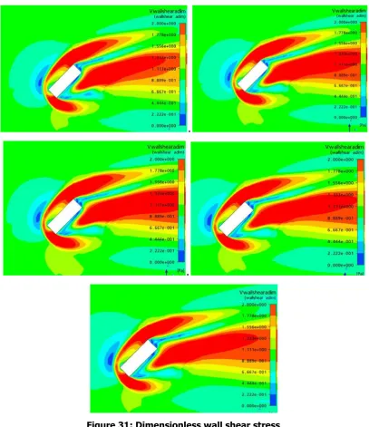
4.3 Boundary thickness effect

The section aims to describe the effect of the boundary thickness on the wall shear. Indeed, the experiment made in wind tunnel often involves a ratio δ/H relatively small (due to the limited wind tunnel length and the smooth material), while the full scale marine structure tend to be submitted to velocity profile with a high δ/H ratio.

(49)

49

The computed boundary layer evolution has been checked by comparing it to the Eq 10 and the agreement is very good.

· 0,38 ·

,

Eq 10

(50)

50

.

[image:50.595.95.503.51.523.2]

.

Figure 31: Dimensionless wall shear stress

(51)

Chapter: Flow and scour around a wreck

51 5-

Flow and scour around a wreck

5.1 Geometry

[image:51.595.103.503.297.730.2]

A scour “prediction” from a CFD result is compared to experimental result [16]. The model studied is a ship which lies on the seabed with different angle of attack. The aim of the calculation is to estimate the scour pattern. The wall shear value would be compared to the threshold of motion of the sand used in the experiment, and the direction of the wall shear could be used to predict the area of deposition.

Figure 32 : Vessel geometry

(52)

52

As no plan was available to describe the ship model used in the experiment, two solutions were available.

• Manual measurement and Maxsurf drawing : This solution would have been long and the result would have been dependent from the measurement quality

• Use 2D pictures of the boat to reconstruct the 3D surface: This method is quick and the result quality is satisfying.

Steps to generate the ship surface:

• Take 2D picture of the model from at least 15 different points of view. A calibration mat is placed under the ship; this allows computing the position of the camera for each shot.

• Correct the lens distortion of the camera by using a photo of a calibration grid • Mask the background on each picture, so that the only visible things are the

calibration mat and the ship. The masking can be performed automatically for almost all pictures if the background is well defined (a good background would be plain). Otherwise, the masking has to be done manually.

• Reconstruct the 3D surface with the software • Export the file to a format readable by ICEM

5.2 Mesh and calculation setup.

The mesh used is unstructured, (tetra + prism layer around the ship and on the seabed); generated with ICEM CFD. As the flow is expected to be steady state, (the flow could be expected to look like the flow around a 5:1 cuboid studied in the previous section) a fine mesh could be used without requiring too big calculation time. The mesh used is therefore about 1 000 000 elements.

(53)

53

• The inlet velocity is a uniform profile; the flow speed is 0.14 m/s

• Re=51000

• median sand grain diameter d₅₀= 0.47mm

• material density ρ_s= 1440kg/m^3

• The roughness of the seabed is approximated by

12

50 0

d

z = = 3.58 e-5 m

The turbulence model used is Shear Stress Transport.

Figure 33 : mesh

5.3 Results

5.3.1 Comparison with the cuboids 5:1.

(54)

54

Figure 34 : visualisation of the vortex structures. Q isosurface. 45 deg

[image:54.595.84.492.70.338.2]

Figure 35 : Wall shear

The general shape of the flow is similar; differences can however be noticed. The maximum wall shear value is closer to the cuboids; although the vortex structure near the trailing edge is not the same.

5.3.2 Roughness effect

(55)

55

for the SST model). To check this assumption, two calculations are run with a k-ε

model, one with a smooth wall and the other with the actual roughness of the sand. The results are very similar (the relative difference is less than 3%).

5.3.3 Wall shear value and threshold of motion.

For slow flows over a seabed, the sand remains immobile, if the flow velocity is increased, the sand would begin to move. At this moment, the threshold of motion is reached. There are several methods for predicting this threshold of motion, for steady flow over a flat seabed; the threshold is often formulated thanks to the current speed. However, as this current study involves structure and complex flow geometry, the more suited measure of the threshold of motion is given in terms of bed shear stress.

The threshold of motion of the sand could by approximated by empirical equation using the Shield criterion [15]:

Dimensionless grain size:

3 / 1 2 *

)

1 (

⎥

⎦

⎤

⎢

⎣

⎡

₋

=

ν

ρ

_s

g

D

Æ D_*= 7.6

Settling velocity:

d

D

w

_s

6

1 . 2 *

⋅

=

υ

_for

₃₉

3

₁₀₀₀₀

*

<

(56)

56

Threshold Shields parameter:

[

0.02 *

]

*

1

055 .

0

2 .

1

30 .

0

D cr

e

D

−

⋅

+

=

θ

_Æ

cr

θ = 0.039

Threshold of motion:

d

g

_s

cr

=

θ

⋅

(

ρ

−

ρ

)

⋅

τ

_Æ

τ

_cr

_{= 0.074 Pa}

5.3.4 Scour onset estimation from CFD result.

This threshold of motion will be compared to the computed wall shear stress for several cases. This would hopefully provide an estimate of the area of erosion.

• Case 1 : Angle of attack 45, alpha = 25 • Case 2 : Angle of attack 90, alpha = 25

5.3.4.1 Case 1

(57)

[image:57.595.163.456.53.281.2]

57

Figure 36 : general view of the flow

[image:57.595.148.456.370.587.2]

(58)

[image:58.595.142.456.57.297.2]

58

Figure 38 : Turbulent kinetic energy just above the seabed.

Figure 39 :Wall shear stress, immobile sand in deep blue. Threshold of motion reached everywhere else.

[image:58.595.140.459.368.588.2]

(59)

[image:59.595.37.524.57.257.2]

59

Figure 40 : Scour prediction

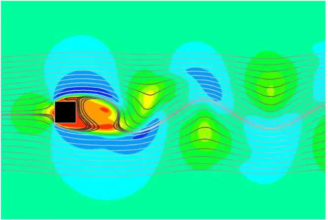
The actual scour map presented on Figure 41 :

Figure 41 : 225 experimental scour patterns

Even if the wall shear map is only the initial map, it allows a relatively good estimate of scour shape. The area of deposition can be expected to be the area where the wall shear is low, next to a high wall shear area oriented toward it. The pit scour regions would simply be the area of high wall shear stress. Obviously this method is an approximation; a precise scour prediction should involve a coupled model. Figure 42 shows the principle of a coupled model. In the current work, the effect of the scour on the flow is not taken into account. Thus only the onset scour could be accurately predicted.

[image:59.595.102.491.273.519.2]

(60)

[image:60.595.138.460.425.655.2]

60

Figure 42 : Coupled model principle

5.3.4.2 Case 2

The first case is a vessel oriented 90 ° toward the flow, lying on the seabed with an angle alpha=25 °. Figure 43 to Figure 46 present the results of the computation.

Figure 43 : Wall shear stress

Flow

computation

Scour

computation

remeshing of

(61)

[image:61.595.140.458.297.524.2]

61

Figure 44 : Velocity just above the seabed

(62)

[image:62.595.135.465.50.517.2]

62

Figure 46 : Streamline

Figure 47 : Wall shear stress

(63)

[image:63.595.128.469.396.606.2]

63

Figure 48 : Experimental scour pattern

However, it can be noticed that the turbulence kinetic just above the seabed matches with the experimental scour map. That was also true for the case 1.

Figure 49 : superimposition scour and TKE.

(64)

64

• The wall shear computed is the mean time wall shear (as the RANS equations

are resolved). The scour processes involving threshold, the turbulence might increase the maximum wall shear stress. However the turbulence kinetic energy is very weak compared to the mean inlet kinetic energy (in this case less than 5%) and thus cannot have such a dramatic effect on the instantaneous wall shear magnitude.

(65)

Chapter: Full scale comparison

65 6-

Full scale comparison

6.1 Configuration

[image:65.595.241.359.264.361.2]

Full scale measurements have been performed by the National Oceanography Centre of Southampton. The study site (Figure 50) is located near the south England coast and is described as “Unknown wreck”. The wreck, which was first recorded in 1918, is about 70 meters long.

Figure 50 : unknown wreck site location

Results about the flow and the scour around the “unknown wreck” are available. This section intends to reproduce the flow around the wreck. The input data are a description of the site topology and the flow measured upstream of the wreck. The description of the topology comes from swath measurements; the resolution of the measurement grid is 0.5 by 0.5 meter.

The topology includes classical bed ripple and a wreck with its actual pit scour.

(66)

[image:66.595.99.499.348.643.2]

66

Figure 51 : Scour on the full scale wreck compared to the turbulence kinetic energy around a cuboid

Although the wreck is only approximately described by the cuboid, a rough match can be observed between the scour shape and the area of high TKE. Next, the actual flow around the actual wreck is simulated for a more precise result. Figure 52 describes the site topology and the probes locations. Figure 53 presents an overview of the flow evolution measured by the probe 1.

(67)

[image:67.595.115.480.64.518.2]

67

Figure 53 : Flow measurement (from [18])

(68)

68

Figure 54 : Mean velocity measured by the probe 1 during a half flood tide.

Figure 55 : Mean direction measured by the probe 1 during a half flood tide.

The velocity measured shows the classical behaviour of the flood tide, the maximum speed being reached in the middle of the half flood tide.

6.2 Whole half flood tide averaging

6.2.1 Input data

As the flow is highly turbulent, the experimental measurements need to be averaged over time; the first simulation will average the velocity profile over nearly the whole half flood tide (i.e. 1h to 5h). The orientation chosen for this simulation is the mean orientation of the flow (i.e. 50 degrees).

0,00 0,10 0,20 0,30 0,40 0,50 0,60 0,70 0,80 0,90

0 2 4 6 8

Ve lo ci ty (m/ s)

Time (hour)

Average velocity

‐150,0 ‐100,0 ‐50,0 0,0 50,0 100,0 150,0 200,0 250,0

0 1 2 3 4 5 6 7 8

Flow

dr

ection

Time

(hour)

(69)

[image:69.595.108.476.84.296.2]

69

Figure 56 : Mean velocity profile, probe 1

It can be noticed that the regression function used to approximate the actual velocity profile matches almost exactly with the empirical relationship (Eq 11 and Eq 12 from [15]). This means that an actual measurement of the inlet velocity is not needed to predict the flow (only the averaged velocity is required).

U

_z

=

1 .

07

For 0.5h < z < h Eq 11

U

h

z

U

_z 7 1

32 .

0 ⎟

⎠

⎞

⎜

⎝

⎛

=

For 0 < z < 0.5h Eq 12

Where z is the height of the reference velocity, Uz and h is the total water depth.

As the inlet of the numerical domain is not actually on the probe 1, the velocity profile at the probe 1 location is checked and matches which the profile expected (Figure 56). The top boundary condition used for this simulation is a free slip wall at 10 meters. Then an opening condition could be tried for more realistic results.

0 0,1 0,2 0,3 0,4 0,5 0,6 0,7 0,8 0,9

‐2 0 2 4 6 8 10

ve lo ci ty (m/ s) Height experiment

adapted power law

empirical law

(70)

70

6.2.2 Results

[image:70.595.100.521.470.717.2]

Velocity profiles:

Figure 57 : probe 6 direction and velocity profile. Averaging during the whole half flood tide

Figure 58 : probe 8 direction velocity profile Averaging during the whole half flood tide

0 2 4 6 8 10 12

0 0,5 1

heigh

t

velocity (m/s)

0 2 4 6 8 10 12

‐50 0 50

Angle

Experiment

Freeslip 10m

0 1 2 3 4 5 6 7 8 9 10

0 0,2 0,4 0,6 0,8

heigh t velocity 0 1 2 3 4 5 6 7 8 9 10

‐10 0 10 20 30

Angle

Experiment

(71)

71

Figure 59 : probe 9 direction velocity profile Averaging during the whole half flood tide

The agreement with the measurement is not that good. The computed results have several weaknesses which could explain partially these disagreements:

• The boundary condition used for the top could be improved; an opening condition would be more suitable.

• As the general flow direction varies during the tide, performing several simulations at different phase of the tide could improve the agreement between the experiment and the simulation. Furthermore, as scour process involve threshold of motion, a calculation on a narrower time range would be more relevant. 0 1 2 3 4 5 6 7 8 9 10

0 0,2 0,4 0,6

Height

Velocity (m/s)

0 1 2 3 4 5 6 7 8 9 10

‐20 0 20 40

(72)

72

The experimental measurement could also be imprecise, the probe 6 is perhaps affected by an offset on the direction (the flow at 10 meters could be expected to be the mean inlet flow direction and it is not). With an offset of 15 °, the computed and measured flow at the probe 6 location would agree.

[image:72.595.106.492.253.462.2]

The following calculation will be performed over a narrower range of time and other boundary conditions will be tested. Two more meshes are thus generated, with a rotation of – 10 and +10 degree. The experimental flow data are now averaged only during the corresponding time.

Figure 60 : Flow direction evolution during the flood tide

6.3 Middle flood tide average

The middle of half-flood tide is the most interesting part from the scour point of view. Indeed, it is during this period that the flow is the strongest; it has also been observed experimentally that the sand was essentially moving during this period (and not during the other period of the flood tide)

Boundary condition tested for the “top” • Free slip wall at 10 meters

• Opening at 10 meters

0,0 20,0 40,0 60,0 80,0 100,0 120,0

0 1 2 3 4 5 6 7

Flow

dr

ection

Time (hour)

Late Middle

(73)

73

Figure 61 shows an overview of the flows (computed with the opening boundary condition) using streamlines starting at different locations.

a )

b)

[image:73.595.193.425.114.694.2]

c)

Figure 61 : streamlines around the wreck

(74)

[image:74.595.79.511.106.567.2]

74

Figure 62 to Figure 64 presents the computed velocity profiles on the probes locations.

Figure 62 : Probe 6 profiles Middle flood tide

Figure 63 : Probe 8 profiles Middle flood tide

0 2 4 6 8 10 12

0 0,5 1

Height

velocity (m/s)

0 2 4 6 8 10 12

‐30 ‐20 ‐10 0 10 20 30

Angle

experiment freeslip10m op 10

0 1 2 3 4 5 6 7 8 9 10

0 0,5 1

heigh t Velocity(m/s) 0 1 2 3 4 5 6 7 8 9 10

‐10 0 10 20 30

Angle

(75)

[image:75.595.109.494.103.452.2]

75

Figure 64 : probe 9 profiles Middle flood tide

The results provided with the opening boundary condition differ significantly from the results with the free slip condition, the agreement with the experiment is better. Concerning the probe 6 angle measurements, an offset could be assumed; the flow direction at 10 meter above the seabed could indeed be expected to be unaffected by the wreck, the direction should then be the inlet direction (that is to says 0 degree instead -15 °).This offset should be the same with the +10° and -10° cases. Furthermore, the probe north reference is set thanks to an internal magnetic compass; the proximity of a big metallic wreck might perturb this compass.

Figure 65 presents result on or near the seabed. Full size pictures are available in appendix 2. 0 1 2 3 4 5 6 7 8 9 10

0 0,5 1

Heigh t Velocity 0 1 2 3 4 5 6 7 8 9 10

‐10 ‐5 0 5 10 15

Angle

(76)

76

a) b)

[image:76.595.81.523.54.507.2]

c) d)

Figure 65 : Turbulence kinetic energy, Depth, Wall shear and velocity plots a)TKE b)depth c)wall shear stress d)velocity

Once again, the wall shear stress fails to locate the deepest scour pit (just behind the wreck), the scour pits match however with the areas of high turbulence kinetic energy.

6.4 Early flood tide average

(77)

[image:77.595.72.520.73.720.2]

77

Figure 66 : probe 6 profiles early flood tide

Figure 67 : Probe 8 profiles

0 1 2 3 4 5 6 7 8 9 10

0 0,5 1

heigh

t

velocity (m/s)

0 1 2 3 4 5 6 7 8 9 10

‐15 ‐10 ‐5 0 5 10

Angle

experiment

openning 10 m

0 1 2 3 4 5 6 7 8 9 10

0 0,2 0,4 0,6 0,8

Heigh

t

velocity (m/s)

0 1 2 3 4 5 6 7 8 9 10

‐10 ‐5 0 5 10 15

Angle

(78)

78

Figure 68 : Probe 9 profiles

The computed and measured profiles match very reasonably (if the assumed offset on probe 6 is removed). Figure 69 presents results on or near the seabed. Full size pictures are available in appendix 2.

0 1 2 3 4 5 6 7 8 9 10

0 0,5 1

Height Velocity 0 1 2 3 4 5 6 7 8 9 10

‐4 ‐2 0 2 4

Angle

experiment

(79)

79

a) b)

c) d)

Figure 69: Turbulence kinetic energy, Depth, Wall shear and velocity plots a)TKE b)depth c)wall shear stress d)velocity

(80)

80

Figure 70

Bottom: middle flood tide / Top: early flood tide Right: velocity / Left: TKE

(81)

81 6.5 Late flood tide average

The same calculation is performed with the late flood tide data; the flow orientation is changed to -10 °.

Figure 71 : probe 6 Late flood tide

0 1 2 3 4 5 6 7 8 9 10

0 0,2 0,4 0,6

Heigh

t

Velocity (m/s)

0 1 2 3 4 5 6 7 8 9 10

‐20 0 20

Angle

(82)

82

Figure 72 : Probe 8 Late flood tide

Figure 73: Probe 9 Late flood tide

0 1 2 3 4 5 6 7 8 9 10

0 0,2 0,4

Heigh t Velocity 0 1 2 3 4 5 6 7 8 9 10

‐5 0 5 10

Angle

Experiment

opening 10m

0 1 2 3 4 5 6 7 8 9 10

0 0,2 0,4

Height

velocity (m/s)

0 1 2 3 4 5 6 7 8 9 10

‐5 0 5 10

angle

(83)

83

a) b)

c) d)

Figure 74 : Turbulence kinetic energy, Depth, Wall shear and velocity plots a)TKE b)depth c)wall shear stress d)velocity

(84)

Chapter: Conclusion

84 7-

Conclusion

It has been shown that the flow around 3D surface mounted structures can be well predicted by RANS CFD analysis, the simplicity of the structure does not correspond to the computing difficulty. Indeed, this work has shown that the flow around a simple cube could be more complex to compute than flow around cuboids with angle of attack or a wreck (due to the vortex shedding effect). For most of the separated flow studied, the turbulence model SST provides acceptable results. For very accurate results for complex flow (for example unsteady flows), SAS-SST model or LES calculation are more suitable. A comparison of computed and measured flow using full scale data is a delicate process, the experimental data does have not a 100% reliability and the computed flow involves an incomplete description (condition as a free surface condition would be computationally too expensive, the domain is truncated by an opening boundary). The moderately good agreement obtained is thus acceptable.

(85)

Chapter: Conclusion

85 R

EFERENCES

[1] W. Rodi. (1997) , Comparison of LES and RANS calculations of the flow around bluff bodies Journal of Wind Engineering and Industrial Aerodynamics 69-71 55 75.

[2] Gianluca Iaccarino and Paul Durbin (2000) “Unsteady 3D RANS simulations using the v2-f Model” Centre for Turbulence Research Annual Research Briefs 2000

[3] Cfx 11 user manual (2006), Ansys

[4] Wilcox, D. C. (1993), Turbulence Modelling for CFD, DCW Industries Inc., La Canada, CA,.

[5] K. Dhinsa, C. Bailey, K. Pericleous, “Investigation into the Performance of Turbulence Models for Fluid Flow and Heat Transfer Phenomena in Electronic Applications”, Centre for Numerical Modelling and Process Analysis, University of Greenwich

[6]. Menter, F. R., "Influence of Free Stream Values on k − ω Turbulence Model Predictions", AIAA Journal, Vol. 30, No. 6, pp. 1657-1659, 1992.

[7]. Menter, F. R., "Improved Two-Equation k − ω Turbulence Model for Aerodynamic Flows", NASA TM- 103975, 1992.

[8] Menter, F. R., "Zonal Two-Equation k − ω Turbulence Models for Aerodynamic Flows", AIAA Technical Paper, 93-2906, 1993.

[9] Nearbed Flow in the Wake of Cuboids: 1. Flow Deflection and Reattachment

D.O. Lambkin, J.K. Dix and S.R. Turnock (in preparation)

[10] W. Rodi, J.E. Cermak et al. “Simulation of flow past buildings with statistical turbulence models” in: (Eds.), Wind Climate in Cities, Kluwer Academic Publishers, Dordrecht, 1995, pp. 649 668.

(86)

Chapter: Conclusion

86

[12] R.J. Pattenden 2004 ‘An investigation of the flow around a truncated cylinder’. PhD Thesis, Faculty of Engineering and Applied sciences, University of Southampton, UK. 182pp

[13] Sklavounos, Fotis Rigas (2004), “Validation of turbulence models in heavy gas dispersion over obstacles.” Spyros School of Chemical Engineering, National Technical University of Athens

[14] Guangchu Hu, Bernard Grossman, “The computation of massively separated flows using compressible vorticity confinement methods”, Computers & Fluids Volume 35, Issue 7, August 2006, Pages 781-789

[15] A simple empirical relationship for typical coastal flows e.g. from Soulsby

(1997) ‘Dynamics of Marine Sands’, Thomas Telford, London, pp249.

[16] Saunders, R.D., 2005. ‘Seabed scour emanating from submerged three-dimensional objects: Archaeological case studies’. PhD Thesis, Department of Civil and Environmental Engineering, University of Southampton, UK. 214pp

[17] Boussinesq, J. (1877), "Théorie de l’Écoulement Tourbillant", Mem. Présentés par Divers Savants Acad. Sci. Inst. Fr., Vol. 23, pp. 46-50.

[18] Field Measurements of Flow Structure Around a Large Submerged 3D Object: The Unknown Wreck, Hastings Shingle Bank, U.K. Journal of Geophysical Research (2006).

[19] Nearbed Flow in the Wake of Cuboids: 2. Flow Deflection and Reattachment

(87)

Chapter: Conclusion

87

(88)

(89)

(90)

Flow and likely scour around three dimensional seabed structures evaluated using RANS CFD

2

Summary

3

Table of contents

4

5

List of Figures

6

7

8

List of Tables

9

10

Introduction

11

12

1-

Computational tools

1.1 Governing equation

·

·

13

0

·

14

·

2

15

16

1.2 RANS Solver details

1.3 Grid generation

17

1.4 Computational resources

18

2-

Preliminary calculations

2.1 Initial study

19

20

21

2.2 2D Calculation with finer meshes

24

25

26

3-

Flow around a surface-mounted cube.

3.1 Geometry and meshes

27

28

3.2 Turbulence model

29

3.3 Time step and simulation time

3.4 Results

30

31

32

33

34

35

36

Q

1

37

38

39

40

41

42

43

4-

Cuboids with different aspect ratio and angle

of attack

4.1 Geometry and input data

4.2 Results

44

45

46

47

48

₋

₃₉

₁₀₀₀₀