School of Human Life Sciences, University of Tasmania, Launceston, Tasmania 7250, Australia, 2
Universiti Kuala Lumpur, Royal College of Medicine Perak, 30450 Ipoh, Perak, Malaysia, 3
Institute of Food, Nutrition and Human Health, Massey University, Palmerston North, New Zealand
[email protected], [email protected], [email protected], [email protected]
Abstract. A common variant of the Michaelis-Menten model of enzyme kinetics involves inhibition by excess substrate. This phenomenon is known as substrate inhibition and the mathematical description of it requires an inhibition constant (Ki) as well as the usual kinetic parameters (Km and Vmax). Fitting the 3-parameter substrate inhibition expression to data that might reasonably be described by the 2-parameter Michaelis-Menten model yields biased estimates of Km and Vmax. Numerical simulations demonstrate that the extent of the bias is related to the magnitude of the estimated Ki. The quality of the data is particularly important in determining the size of Ki and, therefore, in the bias of the other parameters. Consideration of the residuals, statistical justification of the inclusion of extra parameters and reporting of the estimated values should be matters of routine. The estimates of Km and Vmax obtained from a three-parameter substrate inhibition model can only be compared with the corresponding estimates from the two-parameter Michaelis-Menten model with caution.
Keywords: distribution, enzyme kinetics, simulation, substrate inhibition.
1 INTRODUCTION
We have deliberately adapted the title of a paper published in 1978 by Ellis and Duggleby [1] because we have noticed the use of substrate inhibition (SI) models of enzyme kinetics that are not justified by the data [2-4]. This involves analysing data using a three-parameter model rather than the usual two-parameter Michaelis-Menten model (Figure 1). In general, no statistical analysis is given to substantiate the significance of the added parameter which might support the use of such models. In at least some cases, even the most cursory analysis would demonstrate that the extra parameter is not statistically justified.
Figure 1. The mechanism of (A) a Michaelis-Menten enzyme [5] and (B) an enzyme exhibiting substrate inhibition [6]. In each case S, E and P are substrate, enzyme and product, respectively and ES and SES are the enzyme-substrate and substrate-enzyme-substrate complex, respectively. The ki are rate constants, is a factor reflecting the relative rate of P release from SES and Ki is the dissociation constant of SES.
(i) they represent a condition in which SI is eliminated as is the case for ent -copalyl diphosphate synthase [3],
(ii) related enzymes exhibit SI in the conditions employed, as is the case for IMP dehydrogenase [2], and
(iii) related enzymes may exhibit SI in some conditions, as is the case glutamate dehydrogenase [4].
Of these examples, Prisic and Peters [3] have the strongest justification because they report very pronounced SI of ent-copalyl diphosphate synthase (E. C. 5.5.1.13) in the presence of Mg2+, but the activity is considerably reduced and SI is effectively eliminated when Mg2+ is absent. Obviously, these authors wished to compare the kinetic of the enzyme in various conditions, and it might be argued that this necessitates the treatment of the data using an SI model. The latter two situations provide much weaker justification. For example, IMP dehydrogenase (E. C. 1.1.1.205) does exhibit SI in some protozoa (such as Cryptospiridium parvum
[7]), but not in others (such as Leishmania donovani [8]), which makes the assumption of SI in the Toxoplasma gondii enzyme [2] suspect. Similarly, glutamate dehydrogenase (GDH, E. C. 1.4.1.3) can exhibit non-Michaelis-Menten kinetics, including substrate inhibition [9]. While the behaviour of the enzyme can be complicated [10-12], it does depend on the conditions employed. For example, Rife and Cleland [13] pointed out that SI by -ketoglutarate is not apparent in the bovine enzyme at low NH3 concentrations.
The Michaelis-Menten reaction [5] in which an enzyme (E) converts a substrate (S) to a product (P) involves the transient formation of an enzyme-substrate complex (ES) (Figure 1A). The rate of P formation is given by
s K s V s v m M max (1)
where s is the concentration of S, Vmax is the asymptotic value of vM at high s and Km
is sometimes referred to as the ‘affinity’ of the enzyme for S [18]. Equation (1) describes a rectangular hyperbola in which vM increases with s, vM = 0.5Vmax when s = Km and approaches Vmax as s approaches infinity. While there is some argument as to whether any enzyme functions according to this model [19], it does provide a simple means of characterising the kinetic behaviour of many enzymes.
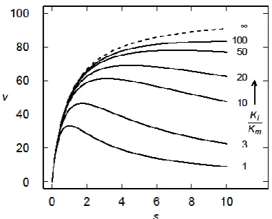
However, the Michaelis-Menten model really does not describe the mechanism of the many enzymes that exhibit SI [9]. In such cases, the initial rise in v with increasing s is followed by a decline in v as s is increased further (Figure 2). A number of mechanisms could give rise to this behaviour, but a simple model in which S may bind to a second site on the enzyme, forming a ternary SES complex (Figure 1B) and thereby eliminating (or at least reducing) the activity of the enzyme is commonly described [6]. This results in a modified Michaelis-Menten equation
s
K
s
K
s
V
s
v
i m S
1
max (2)in which Ki is the dissociation constant of SES (Figure 1B). It is obvious from (2)
that the maximum vS is
max2 K K V
K K K v i m i i m S (3)
and that vS(Km) vS((KmKi)
1/2
). It is not possible to put any useful bounds on the relative magnitudes of Km and Ki. The concentrations at which vS = 0.5vS((KmKi)
Figure 2. Kinetics of the Michaelis-Menten reaction (dashed curve) and substrate inhibition model (solid curves) for several different values of Ki/Km (as indicated). The dashed curve was calculated using (1), but is equivalent to (2) if Ki/Km → ∞, and the other curves were calculated using (2). In all cases Vmax = 100 units and Km = 1 unit.
4 2 6
2 1 5 . 0 m i m i m i m i m K K K K K K K K K s . (4)
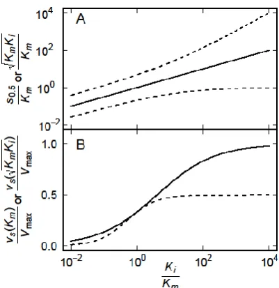
While the two values of s0.5/Km given by (4) exhibit increase with Ki/Km, they
exhibit distinct behaviours (Figure 3). As Ki/Km approaches infinity, the smaller
value approaches 1 whereas the larger value increases monotonically (Figure 3A), reflecting the asymmetry of (2) around the maximum as is apparent in Figure 2. As
Ki/Km approaches infinity, the maximum vS approaches Vmax (3) and vS(Km)
approaches 0.5Vmax, but around Ki/Km = 1 the maximum vS equals vS(Km) (Figure
3B).
3 COMPUTATIONAL METHODS
Experimental data were simulated in R [20] using (1) and a normally distributed random error term (; mean = 0, standard deviation = ) was added to each datum
s
v
s
0
,
v
M , (5)where s = (0, 0.5, 1, 2, 3, 5, 7.5, 10), Vmax = 100 and Km = 1. The error term was
[image:4.595.199.397.139.298.2]Figure 3. Dependence on Ki/Km of (A) the concentration of S yielding maximum vS (solid line) and the concentrations at which vS is half of the maximum values (dashed curves, (4)), and of (B) the maxium vS (solid curve, (3)) and the value of vS(Km) (dashed curve). Note that (KmKi)1/2/Km = (Ki/Km)1/2, but the form used is intended to emphasise the connection with (3).
n j i i M iS s v s
v n 1 8 1 ˆ 8 1 , (6)
where
v
ˆ
S is the fitted value of (2). The magnitude of can be compared with Vmax = 100.We have previously demonstrated the value of a confidence band for (1)
2 2 2max
K
s
V
v
m K V M
(7)[21] and the same approach yields a confidence band () for (2)
2 2 4 2 2 max1
i m I i K V SK
s
s
K
K
s
V
v
(8)where V, K and I are the errors associated with Vmax, Km and Ki, respectively. As
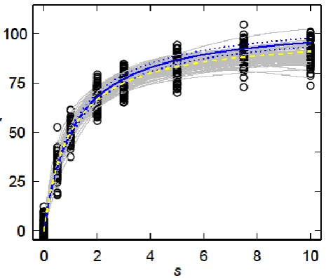
Figure 4. Fits (grey curves) of (2) to simulated data (○) calculated from (5) assuming = 3. The average parameter values (Km, Vmax and Ki) obtained from the fits to each of 100 simulated datasets were used in (2) to calculate the expected curve (solid blue curve) and the associated 95% confidence band (dotted blue curves) were calculated from (8) using the corresponding error estimates (K, V and I). The dashed yellow curve is the Michaelis-Menten curve (1) on which the simulation was based (Vmax = 100 units, Km = 1 unit).
4 NUMERICAL EXPERIMENT
Some representative fits of (2) to simulated data (5) are shown in Figure 4. It is clear that the simulated experimental variation leads to a considerable range of behaviour, including examples in which there is a clear indication of a decline in v
with increasing s (see the lowest grey curve for s = 8-10 units in Figure 4). Using the averages of the n = 100 estimated values of Vmax, Km and Ki in (2) yields an
overestimate of v compared with vM, even when the 95% confidence interval (8) is
taken into account (Figure 4).
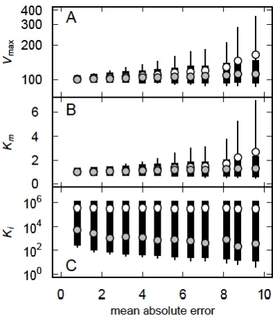
What is not apparent from Figure 4 is the range of parameter estimates obtained even with = 3. A larger number of simulations yields distributions of the parameters (Figure 5). Clearly, there is a strong linear relationship between the estimated values of Km and Vmax (Figure 5A) and both parameters have unimodal distributions (Figures 5, A and B). However, a significant proportion of the simulations yielded parameter estimates that were much larger than the actual values (Vmax = 100 units, Km = 1 unit) and a smaller proportion of the estimates were
increasing (Figure 6). The bimodal distribution of Ki is clear because the mean is
largely unaffected by changes in , whereas the median declined with increasing (Figure 6C).
5 DISCUSSION
The unjustified use of (2) rather than (1) can distort the estimates of Vmax and Km
obtained. In general, this tends to yield overestimates of Vmax and Km, especially if
experimental error is sufficient to result in estimates of Ki < 10
3
[image:7.595.119.478.478.634.2]Figure 5. Distributions and relationships between the parameter estimates (○) obtained from fitting (2) to each of 10000 simulations of (5). (A) The relationship between the estimates of Vmax
and Km and the distribution of Vmax (upper histogram). (B) The relationship between the estimates
of Km and log10(Ki) and the distribution of Km (upper histogram). (C) The relationship between the estimates of Vmax and log10(Ki) and the distribution of log10(Ki) (upper histogram). It was assumed that Vmax = 100 units, Km = 1 unit and = 3.
Figure 6. Effect of error on the distributions of the estimates of Vmsc (A), Km (B) and Ki (C) obtained by fitting (2) to data simulated using (5). In each case the solid black column represents the 25th-75th percentiles, the line extends from the 5th to the 95th percentile and the open (○) and
grey (●) circles represent the mean and median, respectively.
In passing, we suggest that the inappropriate use of SI models is partly promoted by their availability in popular software packages such as Prism, which was used in two of the three examples we outlined in the introduction [2, 4]. Another common source of bias in parameter estimates [23, 24] is the use of the double-reciprocal plot proposed by Lineweaver and Burk in 1934 [22]. We speculate that the widespread use of software of this sort promotes the continued application of such transformations despite the statistical arguments in favour of the use of nonlinear regression [25] and the availability of the necessary software [20].
[image:8.595.196.395.245.474.2]equation?" Biochemical Journal 1978; 171: 513-517.
2. Sullivan, WJ, Jr, Dixon, SE, Li, C, Striepen, B and Queener, SF, "IMP dehydrogenase from the protozoan parasite Toxoplasma gondii", Antimicrobial Agents and Chemotherapy 2005; 49: 2172-2179.
3. Prisic, S and Peters, RJ, "Synergistic substrate inhibition of ent-copalyl diphosphate synthase: a potential feed-forward inhibition mechanism limiting gibberellin metabolism", Plant Physiology 2007; 144: 445-454.
4. Umair, S, Knight, JS, Patchett, ML, Bland, RJ and Simpson, HV, "Molecular and biochemical characterisation of a Teladorsagia circumcincta glutamate dehydrogenase", Experimental Parasitology 2011; 129: 240-246.
5. Michaelis, L and Menten, ML, "Die Kinetik der Invertinwirkung", Biochemische Zeitschrift 1913; 49: 333-369.
6. Haldane, JBS, "Enzymes", Longmans, Green and Co., London. 1930.
7. Umejiego, NN, Li, C, Riera, T, Hedstrom, L and Striepen, B, "Cryptosporidium parvum
IMP dehydrogenase. Identification of functional, structural, and dynamic properties that can be exploited for drug design", Journal of Biological Chemistry 2004; 279: 40320-40327.
8. Dobie, F, Berg, A, Boitz, JM and Jardim, A, "Kinetic characterization of inosine monophosphate dehydrogenase of Leishmania donovani", Molecular and Biochemical Parasitology 2007; 151: 11-21.
9. Reed, MC, Lieb, A and Nijhout, HF, "The biological significance of substrate inhibition: a mechanism with diverse functions", BioEssays 2010; 32: 422-429.
10. Hudson, RC and Daniel, RM, "L-Glutamate dehydrogenases: distribution, properties and mechanism", Comparative Biochemistry and Physiology 1993; 106B: 767-792.
11. Kurganov, BI, "New approach to analysis of deviations from hyperbolic law in enzyme kinetics", Biokhimiya 2000; 65: 898-909.
12. Smith, TJ and Stanley, CA, "Untangling the glutamate dehydrogenase allosteric nightmare", Trends in Biochemical Sciences 2008; 33: 557-564.
13. Rife, JE and Cleland, WW, "Kinetic mechanism of glutamate dehydrogenase", Biochemistry 1980; 19: 2321-2328.
14. Muhamad, N, Brown, S, Pedley, KC and Simpson, HV, "Kinetics of glutamate dehydrogenase from L3 Ostertagia circumcincta", New Zealand Journal of Zoology 2004; 31: 97.
16. Akaike, H, "A new look at the statistical model identification", IEEE Transactions on Automatic Control 1974; 19: 716-723.
17. Bardsley, WG, McGinlay, PB and Wright, AJ, "The F test for model discrimination with exponential functions", Biometrika 1986; 73: 501-508.
18. Briggs, GE and Haldane, JBS, "A note on the kinetics of enzyme action", Biochemical Journal 1925; 19: 338-339.
19. Hill, CM, Waight, RD and Bardsley, WG, "Does any enzyme follow the Michaelis-Menten equation?" Molecular and Cellular Biochemistry 1977; 15: 173-178.
20. Ihaka, R and Gentleman, R, "R: a language for data analysis and graphics", Journal of Computational and Graphical Statistics 1996; 5: 299-314.
21. Brown, S, Muhamad, N, Pedley, KC and Simcock, DC, "A simple confidence band for the Michaelis-Menten equation", International Journal of Emerging Sciences 2012; 2: 238-246.
22. Lineweaver, H and Burk, D, "The determination of enzyme dissociation constants", Journal of the American Chemical Society 1934; 56: 658-666.
23. Dowd, JE and Riggs, DS, "A comparison of estimates of Michaelis-Menten kinetic constants from various linear transformations", Journal of Biological Chemistry 1965; 240: 863-869.
24. Blunck, M and Mommsen, TP, "Systematic errors in fitting linear transformations of the Michaelis-Menten equation", Biometrika 1978; 65: 363-368.
![Figure 1. The mechanism of (A) a Michaelis-Menten enzyme [5] and (B) an enzyme exhibiting substrate inhibition [6]](https://thumb-us.123doks.com/thumbv2/123dok_us/156012.33156/2.595.226.367.143.235/figure-mechanism-michaelis-menten-enzyme-exhibiting-substrate-inhibition.webp)
![Figure 2. It is a simple matter to determine whether the introduction of an extra parameter is statistically justified [16, 17], but this tends not to be done [2, 4] and it is difficult to assess without access to the data](https://thumb-us.123doks.com/thumbv2/123dok_us/156012.33156/7.595.119.478.478.634/figure-simple-determine-introduction-parameter-statistically-justified-difficult.webp)