Thesis by
Pengfei Sui
In Partial Fulfillment of the Requirements for the Degree of
Doctor of Philosophy
CALIFORNIA INSTITUTE OF TECHNOLOGY Pasadena, California
2018
© 2018 Pengfei Sui
ACKNOWLEDGEMENTS
I am indebted to a great many people who accompanied me along this journey.
First, I am deeply grateful to my committee members, Lawrence Jin, Jakša Cvitani´c, Matthew Shum, and Colin Camerer, for their enormous support and endless encour-agement. Their knowledge and wisdom, their attitude towards research, and their personality have always been inspiring me.
I owe special thanks to my aunt Suhua Dong, and my cousin Jianjie Li, for their patience and support. I am also indebted to my friends, Haoyao Liu, Cong Wang, Wenguang Wang, Dayin Zhang, Seo Young (Silvia) Kim, Xiaomin Li, Yimeng Li, and Jun Zhang, for their company.
I thank the division faculty and staff, especially Jean-Laurent Rosenthal, Michael Ewens, Ben Gillen, Thomas Palfrey, Bob Sherman, Philip Hoffman, Marina Agra-nov, and Antonio Rangel, for their invaluable suggestions. I am grateful to Laurel Auchampaugh and Sabrina De Jaegher for their incredible assistance and support. I am also thankful to Jun Chen, Lucas Nunez, Alejandro Robinson Cortes, Mali Zhang, and Marcelo Fernandez, who helped make this five years memorable.
ABSTRACT
This dissertation is composed of three chapters addressing the connections between investor beliefs and asset pricing. Specifically, I focus on one prevailing pattern of investor beliefs in the finance literature, return extrapolation. The idea is that investor expectations about future market returns are a positive function of the recent past returns. In this dissertation, I use this concept to understand a number of facts in the asset pricing literature.
Return extrapolation attracts growing attention in the literature, not only because it well explains real-world investors’ expectations in the survey, but also because it sig-nificantly drives investor demand towards stocks. Therefore, we should anticipate a connection between return extrapolation measurement and the stock market dynam-ics. However, contrary to the intuition, previous empirical studies fail to document a significant connection. In Chapter 1, “Time-varying Impact of Investor Sentiment”, I recover this connection. Specifically, I formally define investors who extrapolate past returns as extrapolators and incorporate their wealth level into analysis. My main finding is that return extrapolation interacts strongly with extrapolators’ wealth level in predicting future market returns. Therefore, conditional on extrapolators’ wealth level, return extrapolation significantly explains stock market returns.
TABLE OF CONTENTS
Acknowledgements . . . iv
Abstract . . . v
Table of Contents . . . vii
List of Illustrations . . . ix
List of Tables . . . x
Chapter I: Time-varying Impact of Investor Sentiment . . . 1
1.1 Introduction . . . 1
1.2 Motivating Facts . . . 7
1.3 The Behavioral Model . . . 14
1.4 Model Implications . . . 27
1.5 The Role of Extrapolation: A Rational Benchmark Model . . . 36
1.6 Concluding Remarks . . . 42
Chapter II: Asset Pricing with Return Extrapolation . . . 43
2.1 Introduction . . . 43
2.2 The Model . . . 49
2.3 Model Implications . . . 58
2.4 Comparative Statics . . . 72
2.5 Comparison with Rational Expectations Models . . . 75
2.6 Fundamental Extrapolation . . . 78
2.7 Conclusion . . . 81
Chapter III: “Dark Matter” of Finance in the Survey . . . 83
3.1 Introduction . . . 83
3.2 Data . . . 88
3.3 Consistency between Two Types of Surveys . . . 93
3.4 Connections between Return Extrapolation and Perceived Left-tail Probabilities . . . 97
3.5 Concluding Remarks . . . 101
Bibliography . . . 103
Appendix A: Appendix to Chapter One . . . 110
A.1 Micro-foundations for Fundamental Investors . . . 110
A.2 Rational Benchmark Model . . . 112
A.3 Behavioral Model . . . 114
A.4 Figures and Tables . . . 121
A.5 Alternative Regressions . . . 145
Appendix B: Appendix to Chapter Two . . . 151
B.1 Derivation of the Differential Equations . . . 151
B.2 Numerical Procedure for Solving the Equilibrium . . . 153
LIST OF ILLUSTRATIONS
Number Page
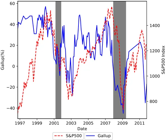
A.1 Gallup Investor Expectations and S&P 500 Index . . . 121
A.2 Gallup Investor Expectations and Household Mutual Fund Flows . . 122
A.3 Predictive Power of Investor Sentiment: Intuition . . . 123
A.4 Calibrated Model Solutions: Rational Benchmark. . . 124
A.5 Calibrated Model Solutions: Behavioral Model. . . 125
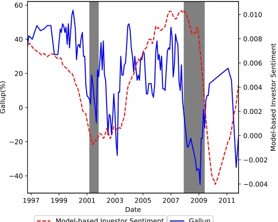
A.6 Gallup Survey and Simulated Investor Sentiment. . . 126
A.7 Interaction between Wealth and Investor Sentiment vs Degree of Extrapolation. . . 127
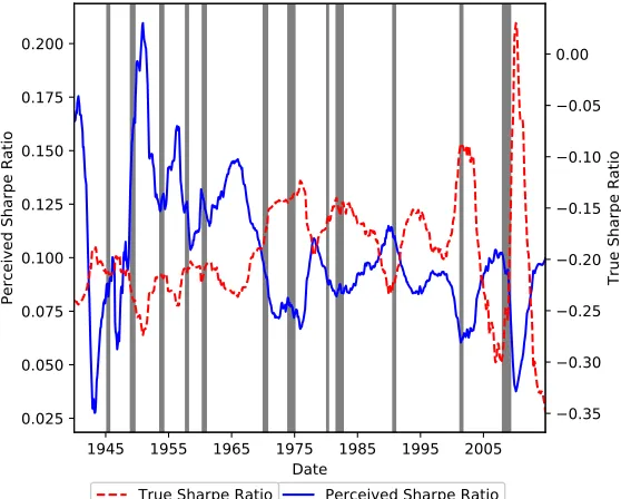
A.8 Perceived Sharpe Ratio and True Sharpe Ratio. . . 128
B.1 Important Equilibrium Quantities Each as a Function of Sentiment. . 157
B.2 Objectively Measured Steady-State Distribution of Sentiment. . . 158
B.3 Objective and Subjective Expectations about Price Growth. . . 159
B.4 Agent’s Expectations about Stock Market Returns, Price Growth, and Dividend Growth. . . 160
B.5 Comparative Statics: Utility Parameters. . . 161
B.6a Comparative Statics: Belief Parameters (I). . . 162
B.6b Comparative Statics: Belief Parameters (II). . . 163
C.1 Tail Risk Measurements Based on Shiller Tail Risks Survey. . . 182
C.2 Connecting Investor Expectations with Perceived Left-tail Risks. . . . 183
LIST OF TABLES
Number Page
A.1 Summary Statistics . . . 129
A.2 Forecast Revision of Investor Sentiment . . . 130
A.3 Predictive Regressions on Future Returns . . . 131
A.4 Conditional Predictive Regressions on Future Returns . . . 132
A.5 Conditional Predictive Regressions on Future Returns (with Controls) 133 A.6 Parameter Values . . . 134
A.7 Simulated Extrapolative Expectations: Behavioral Models . . . 135
A.8 Memory Structure of Investor Expectations: Behavioral Models . . . 136
A.9 Forecast Revision of Investor Sentiment: Simulated Results Based on Behavioral Model . . . 137
A.10 Model-simulated Conditional Predictive Regressions on Future Re-turns: Behavioral Models . . . 138
A.11 Conditional Predictive Power of Investor Sentiment. . . 139
A.12 Conditional Predictive Power of Investor Sentiment: Simulations based on the Behavioral Models. . . 140
A.13 Leverage Ratio and Future Consumption Growth: Behavioral Models 141 A.14 Simulated Extrapolative Expectations: Rational Benchmark Models . 142 A.15 Model-simulated Conditional Predictive Regressions on Future Re-turns: Rational Benchmark Models . . . 143
A.16 Leverage Ratio and Future Consumption Growth: Rational Models . 144 A.17 Conditional Predictive Regressions on Future Returns . . . 146
A.18 Conditional Predictive Regressions on Future Returns (With Controls)147 A.19 Model-simulated Conditional Predictive Regressions on Future Re-turns: Behavioral Models . . . 148
A.20 Conditional Predictive Power of Investor Sentiment. . . 149
A.21 Conditional Predictive Power of Investor Sentiment: Simulations based on the Behavioral Models. . . 150
B.1 Investor Expectations. . . 164
B.2 Determinants of Investor Expectations. . . 166
B.3 Parameter Values. . . 168
B.4 Basic Moments. . . 169
B.5 Return Predictability Regressions. . . 170
B.7 Campbell-Shiller Decomposition. . . 172 B.8 Autocorrelations of Log Excess Returns and Log Price-dividend Ratios.173 B.9 Return Predictability Regressions in the True Regime-Switching Model.174 B.10 Investor Expectations in Bansal and Yaron (2004). . . 175 B.11 Investor Expectations in Bansal et al. (2012). . . 177 B.12 Investor Expectations in the Fundamental Extrapolation Model. . . . 179 B.13 Basic Moments in the Fundamental Extrapolation Model. . . 181
C.1 Summary Statistics and Correlations between Investor Expectation Surveys . . . 185 C.2 Correlations between the Left-tail Probabilities from Investor
Expec-tation Surveys. . . 186 C.3 Contemporaneous Connections between Shiller Left-tail Probability
and Investor Expectations: Individual Investors . . . 187 C.4 Contemporaneous Connections between Shiller Left-tail Probability
and Investor Expectations: Institutional Investors . . . 188 C.5 Left-tail Probabilities based on Return Extrapolation and Rational
Expectations (with VIX). . . 189 C.6 Left-tail Probabilities based on return extrapolation and rational
C h a p t e r 1
TIME-VARYING IMPACT OF INVESTOR SENTIMENT
1.1 Introduction
Whether investor sentiment influences the market has been a long-standing question in the finance literature. From the Great Crash in 1929 to the Internet bubble, from the Nifty Fifty bubble to the 2008 financial crisis, each of these episodes is asso-ciated with dramatic changes in asset prices. Traditional finance theories—models in which investors have fully correct beliefs about the asset dynamics and therefore always force the asset prices to the rational present value of expected future cash flows—leave no room for investor sentiment and have considerable difficulty fitting these patterns. However, investor sentiment, which reflects excessive optimism and pessimism in investor beliefs, seems to play a central role in these phenomena. The large gap between the traditional models and the salient market episodes with dra-matic asset price movements has made researchers realize thatbelief-basedinvestor sentiment plays an important role in asset pricing dynamics.
Relying on survey evidence, recent studies have highlighted the concept of extrapolation— making forecasts about future returns based on past realized returns—in understand-ing the dynamics of investor beliefs. Extrapolation implies that investors tend to believe that asset prices continue to increase after a sequence of high returns and fall after a sequence of low returns (Greenwood and Shleifer (2014)), and has been used to account for the excessive optimism and pessimism in the market (? and Barberis).1 As a result, in this paper, I use extrapolation to characterize belief-based investor sentiment. But despite its prevalence in surveys and its importance in investors’ portfolio choice, there is no strong empirical evidence that belief-based investor sentiment influences the aggregate stock market. In other words, extrap-olation alone leaves the impact of investor sentiment unsolved: for instance, in Greenwood and Shleifer (2014), investor beliefs reported in the survey have only insignificant predictive power over future aggregate stock market returns.
In this paper, I provide a parsimonious approach to reveal the impact of
based investor sentiment. By incorporating the time-varying market impact of extrapolation, which is a notion largely overlooked by the literature, this paper documents and highlights the impact of belief-based investor sentiment on the aggregate market. Specifically, in addition to the basic extrapolation framework, I incorporate the wealth dynamics of investors who extrapolate to proxy for the market impact of extrapolation. In this setting, extrapolation and its market impact together drive the asset price dynamics: when the market impact of extrapolation is high, extrapolation induces irrational demand for the risky asset and, therefore, it leads to mispricing; when the market impact is low, extrapolation simply reflects the recent market dynamics. The interaction between extrapolation and its market impact sheds new light on asset mispricings. More importantly, although investor beliefs alone do not significantly predict future aggregate market returns, they have salient predictive power after conditioning on their market impact—a result that supports both my model implications and my empirical exercise. This conditional predictive power of investor sentiment not only provides direct evidence of the impact of investor beliefs on the aggregate stock market, it also helps to reveal the underlying mechanism of the predictability of returns.
To formalize these arguments, I first develop a continuous-time dynamic equilib-rium model that features two types of investors: extrapolators and fundamental investors. On the basis of past price changes, extrapolators forminvestor sentiment, or, equivalently, their perceived expectation about future risky asset returns, and they make an investment choice between a risky and risk-free asset. After consecu-tive posiconsecu-tive price changes in the past, extrapolators become optimistic about future returns, and after a streak of negative price changes, they become pessimistic about future returns. However, the perceived expectations are different from the true ones and, therefore, high or low investor sentiment, in general, cannot continue for long since extrapolators will easily become disappointed by shocks in the future. Conse-quently, investor sentiment reverts to its mean. Moreover, the major departure from previous extrapolation models is to incorporate the wealth level of extrapolators: all other things being equal, extrapolators have a larger impact on the equilibrium asset prices when their wealth level is higher.
lean against the wind and push prices upwards. However, their ability to correct mispricing depends on the wealth level of extrapolators: fundamental investors can easily correct mispricing when sentiment-driven wealth is low, while the correction takes longer when the wealth level of extrapolators is high.
This model setting generates the key result: when their wealth level is high, ex-trapolators drive the asset prices. In this case, high investor sentiment makes the current asset price overvalued, and the future asset price will decline because high investor sentiment will cool down over time. Therefore, investor sentiment nega-tively predicts future market returns. Conversely, when the wealth level is low, high investor sentiment predicts high future returns because the market is under a price correction. This predictive power of investor sentiment provides direct theoretical support for my conclusion that investor beliefs impact the aggregate stock market.
Moreover, this predictive power supports belief-based explanations of the pre-dictability of returns—that prices temporarily deviate from the level warranted by fundamentals because of the existence of extrapolators, but they revert back as a mispricing correction gradually takes place in the future. Cassella and Gulen (2015) provide empirical support for this explanation. They define the degree of extrap-olation (DOX) as the relative weight extrapolators place on recent-versus-distant past returns when they form subjective expectations for future asset returns. When DOX is high and, therefore, when investor beliefs are transitory, mispricings are corrected more quickly and price-scaled variables (such as price-to-dividend ratio) have stronger predictive power. One possible determinant of the variations in DOX is the time-varying consensus level of extrapolation among market participants. In my model, the time-varying wealth level of extrapolators effectively drives the consensus level of extrapolation in the market.
My model matches other salient patterns in the asset pricing literature. For instance, the mean-reversion of investor sentiment naturally generates a negative equity pre-mium when investor sentiment is high, a pattern that is consistent with findings documented by Baron and Xiong (2017). The fact that my model generates a nega-tive correlation between investors’ expectations and the subsequent realized returns is consistent with the findings of Greenwood and Shleifer (2014). Moreover, the resulting countercyclical Sharpe ratio is consistent with empirical evidence doc-umented by Lettau and Ludvigson (2010). All these asset pricing patterns seem puzzling under a rational expectations framework.
the CRSP value-weighted index and Gallup survey data. During the period of December 1996 to September 2011, Gallup asked individual investors to report their expectations of aggregate stock market returns in the next twelve months. Using these responses I measure investors’ perceived expectations directly. As a robustness check, I also follow Barberis et al. (2015) and construct an investor sentiment index, Psentiment, that is purely based on extrapolation.2 Moreover, Gallup survey evidence helps to identify extrapolator groups, which allows me to select a reasonable proxy for the wealth level of extrapolators.
To find reasonable measurements for extrapolators, I focus on the “Households and Non-Profitable Organizations” (HNPO hereafter) sector reported in the “Financial Accounts of the United States”. Investors in this sector generally are individual investors who are less sophisticated than institutional investors. Moreover, Yang and Zhang (2017) document, first, that investor sentiment in the survey effectively drives the portfolio position of investors in stocks in the HNPO sector and, second, that such sentiment-driven investment negatively predicts returns in the following quarters.3 Their analysis effectively indicates that investor beliefs in the HNPO sector are associated with extrapolation. My model therefore uses the total financial assets of the HNPO sector as the proxy for the wealth level of extrapolators.
My empirical tests support the main predictions of my model. Specifically, I construct an interaction term between the Gallup survey expectations and wealth dividend ratios in the HNPO sector, and I use it to predict future market returns. I find a statistically significant and negative coefficient for the interaction term, which indicates that investor sentiment connects closely to market mispricing when the wealth level of extrapolators is high. This result holds over different predictive horizons, ranging from one to six quarters.
Furthermore, following Aiken et al. (1991), I empirically present the predictive pattern of investor sentiment conditional on different wealth levels of extrapola-tors.When the wealth level of extrapolator is two standard deviation above its mean, one standard deviation increase in investor sentiment measured by the Gallup sur-vey is followed by a significant decrease of 16.2% in future twelve-months returns. This is consistent with my model implication: when extrapolators drive the market,
2In my empirical analysis, I use both survey evidence and Psentiment to test my model predic-tions. If investor beliefs in the survey are mainly driven by extrapolation, then two pieces of parallel evidence should yield similar results for most of my tests. This point is strongly confirmed in my exercise.
investor sentiment reverts to its mean and leads to a negative predictive sign. This pattern remains valid when Psentiment replaces Gallup. Conversely, when extrapo-lators’ wealth level is two standard deviation below its mean, one standard deviation increase in investor sentiment predicts a striking future market return of 35.9%: as my model implies, when sentiment-driven wealth is low, investor sentiment reflects the market valuation correction and, therefore, it positively predicts future market returns.
Implications for the Literature. This paper belongs to the burgeoning return extrapolation literature. Many works in this field try to understand the role that return extrapolation plays in the aggregate stock market. (Cutler et al. (1990b), De Long et al. (1990), Barberis et al. (2015) and Jin and Sui (2017)). Barberis et al. (2015) use return extrapolation to construct an asset pricing model that can explain central asset pricing facts such as the excess volatility puzzle, the predictability of returns, and the investor belief survey evidence in the data. Jin and Sui (2017) construct a quantitative benchmark of belief-based asset pricing models that can simultaneously explain the equity premium puzzle, the excess volatility puzzle, the predictability of returns, the low correlations between consumption and returns, and investor belief evidence in the surveys. However, all existing studies of return extrapolation ignore the role that the wealth level of extrapolators plays in asset dynamics. By incorporating the wealth dynamics of extrapolators and the counteracting forces from fundamental investors, I document a novel predictive pattern for future stock market returns.
This paper also relates to the idea of limits to arbitrage, which is one of the founda-tions for the behavioral finance literature. In its pioneer work, Shleifer and Vishny (1997) argue that asset mispricing may exist for a long time because arbitrage ac-tivities are limited. This is especially true when investment is delegated to portfolio managers with short investment horizons and when the arbitrage activities face noise trader risk and other risks. Abreu and Brunnermeier (2002) provide an additional argument for limited arbitrage.4 My paper utilizes the concept of limits to arbi-trage in a less direct way. Instead of focusing on the agency issue and risks for the arbitragers, I mainly focus on the belief dynamics and the relative market impact of noise traders. When their wealth level is high, arbitragers effectively face more difficulties correcting the mispricing. In addition, by focusing on extrapolators, I can not only provide a specific belief pattern for noise traders but also document a
salient impact of investor beliefs on the aggregate stock market.
This paper is also relevant to the return predictability literature. Previous stud-ies have suggested that aggregate stock returns are predictable using price-scaled variables, such as the dividend-to-price ratio and the earning-to-price ratio (Fama and French (1988), Campbell and Shiller (1988), and Cochrane (2011)). Some researchers attribute the predictability of stock market returns to variations in in-vestors’ required returns. However, behavioral theoretical models attribute the predictability to mispricings induced by investors’ biased beliefs (Barberis et al. (2015), Hirshleifer et al. (2015), and Jin and Sui (2017)). Bacchetta et al. (2009) document that the predictability of excess returns is often associated with the pre-dictability of expectational errors, and this conclusion holds true for a broad set of asset classes, including the stock, foreign exchange and bond assets. Moreover, Cassella and Gulen (2015) empirically investigate the extent to which biased beliefs can help explain the observed predictability in the data. In this paper, I connect investor sentiment with return predictability through the time-varying impact of extrapolators and find empirical support for this result.
This paper also contributes to the literature that examines the impact of investor sentiment. Baker and Wurgler (2006) construct the investor sentiment index by directly using the first principal component of important market indicators, such as volume and equity share issuance, and demonstrate that investor sentiment has a large impact on the cross-section of stock returns. Baker and Stein (2004) propose an investor sentiment index based on market liquidity, and they show that it has predictive power for future market returns. Stambaugh et al. (2012), who also use the sentiment index provided by Baker and Wurgler (2006), find that overpricing is more prevalent than underpricing when market-wide sentiment is high. However, most of these studies construct investor sentiment using a “top down” approach, which employs reduced-form variations in investor sentiment over time. By contrast, this paper uses a “bottom up” approach, and it focuses on the belief formation of investors. My focus on the microfoundations of the variation in investor sentiment allows me to shed new light on the dynamic patterns of the investor sentiment index. Like the “top down” literature, my analysis shows that investor sentiment has a large impact on the aggregate stock market.
market booms and often leads to severe financial crashes. He and Krishnamurthy (2008) also propose a model that generates a procyclical leverage ratio that is based on financial intermediations. This model also helps generate a procyclical leverage ratio. However, in contrast to previous studies, in my model the procyclicality arises from extrapolation. During market booms, extrapolators become overly optimistic because they extrapolate the past returns and, consequently, they buy more risky assets. Conversely, during recessions, extrapolators become overly pessimistic and, therefore, they have a low leverage level. Second, extrapolation also helps explain the nagative association between household leverage and future consumption growth documented in Mian and Sufi (2009). Extrapolation induces investors to make unreasonable investment decisions that lead to a future decrease in wealth, which pushes down consumption growth rate.
Outline: This paper is organized as follows. In Section 1.2, I document some dynamics of belief-based investor sentiment and identify the group of investors who are more susceptible to extrapolation. In Section 1.3, I construct a behavioral model that incorporates both extrapolation and the wealth dynamics of extrapolators. Then I derive several model predictions about the time-varying impact of investor sentiment. In Section 1.4, I examine these model predictions via both simulation and data analysis. In Section 1.5, I examine the role of extrapolation by considering a rational model as the benchmark. Section 1.6 summarizes results and proposes directions for future research.
1.2 Motivating Facts
The difficulty of investigating the impact of belief-based investor sentiment lies both in how to correctly measure investor beliefs and how to measure its overall market impact. To provide insights into the dynamics of belief-based investor sentiment, I resort to investor expectation surveys which directly asks investors about their beliefs. In my later analysis, I will use two terms—belief-based investor sentiment and survey measurement of investor sentiment—interchangeably whenever there is no confusion. Further, relying on survey measurements of investor sentiment, I identify one specific group of investors who tend to extrapolate so that I can measure the market impact of extrapolators properly.
Investor Sentiment Dynamics
respondents are asked about their expectations on future market returns, ranging from six to twelve months. Compared to other measurements of investor expecta-tions, survey measurements are more direct in extracting investor belief information.
In this paper, I mainly use the Gallup survey which measures individual investors’ expectations of the U.S. stock market over the next twelve months.5 It is conducted monthly between 1996 and 2011, but there are some gaps in later years especially between November 2009 and February 2011 when the survey was discontinued. To extract investor expectations, in each month, Gallup survey asks participants one
qualitative question: whether they are “very optimistic”, “optimistic”, “neutral”, “pessimistic”, “very pessimistic” about stock returns over the next twelve months. With the percentage of each response in the collected survey answers, Gallup reports a qualitative investor expectation series to measure investor expectations in the market:
Gallup= %Bullish−%Bearish, (1.1)
where “Bullish” is defined as either “very optimistic” or “optimistic” and “Bearish” is defined as either “pessimistic” or “very pessimistic”. This qualitative time series helps us understand the dynamics of investor sentiment in the market. Moreover, Gallup survey also asks more precise quantitative questions about investors’ per-ceived expected returns, although only for a shorter sample. Specifically, between September 1998 and May 2003, Gallup asks participants to give an estimate of the percentage return they expect for the stock market over the next year. Therefore, as long as participants in the Gallup survey answer quantitative and qualitative questions in a consistent way, I can effectively get quantitative estimations investor expectation series by rescaling qualitative Gallup investor series with projection method.6 This projection method also helps me transform qualitative series in other investor expectation surveys to a meaningful quantitative basis.
However, there were two main concerns about the survey data. One concern is that survey evidence is imprecisely measured and thus is noisy. The other is that survey respondents may be confused by the sophisticated questions and therefore could not
5I use Gallup survey measurement to measure investor sentiment since Gallup mainly surveys individual investors who are more likely to extrapolate. Moreover, Gallup survey has a quantitative measurement of investor expectations to facilitate my analysis.
provide pertinent answers. Fortunately, there are recent developments that show the validity of the investor survey information. Greenwood and Shleifer (2014), among other findings, show that (1) information contained in different surveys reflects sim-ilar patterns and (2) the reported investor expectations in the surveys are largely consistent with investors’ behaviors (See Figure A.2).7 Their findings indicate that survey measures of investor expectations are not meaningless noise but represent widely shared beliefs about future returns in the stock market. With these validations from previous literature, I report the following observations to motivate my model.
Observation 1. Survey measurement of investor sentiment is positively associated with the past returns in the aggregate stock market.
Observation 1 is the main message in Greenwood and Shleifer (2014), and is a restatement of extrapolation: investors in the surveys over-extrapolate recent returns when forming their expectations in their minds. Formally, I useextrapolatorsto re-fer to these investors. Therefore, past good returns tend to make extrapolators overly optimistic while past bad returns make them overly pessimistic. For the underlying psychological mechanisms of extrapolation, there are several candidate theories, including representativeness. Kahneman and Tversky (1972) define representative-ness as “the degree to which an event (i) is similar in essential characteristics to its parent population, and (ii) reflects the salient features of the process by which it is generated”.8 With representativeness, extrapolators might mistakenly treat a sequence of good (bad) recent returns as a salient feature of the whole distribution of returns, which leads to an over-extrapolation. Although the fact that extrap-olators overweight information in the recent returns is commonly documented in recent empirical studies (Amromin and Sharpe (2013), Bacchetta et al. (2009) and Greenwood and Shleifer (2014)), the source of over-extrapolation still remains an important open question.
The belief-based investor sentiment in the surveys is consistent with most of the anecdotal fluctuations of investor sentiment—that investor sentiment rise rapidly
7For result one, the authors compare survey sources from the American Association of Indi-vidual Investors (AA), Gallup, Graham and Harvey, Investors’ Intelligence newsletter expectations, Michigan Survey and Shiller, and document strong correlations between each survey. For result two, the authors examine the reported investor expectations and the investor mutual fund flows, and find two time-series are highly synchronized.
during booms and decrease during crash episodes—in the market. In Figure A.1, I plot the Gallup survey measurement of investor sentiment, ranging from 1996:12 to 2011:09, with the backdrop of shaded NBER recessions. During the “Internet Bubble” episodes in mid-2000, Gallup survey measurement of investor sentiment rises to its peak but drops dramatically after the burst. Similarly, Gallup survey measurement rebounds to the peak before the 2007 financial crisis and declines significantly after the market index fell in 2008.
[Place Table A.1 about here]
To further reveal the close connections between investor sentiment in the survey and extrapolation, I construct a new investor sentiment variable called “Psentiment”. Previous studies on the belief patterns in the survey indicate that when forming beliefs on expectations of returns, extrapolators put a decaying weight on the realized returns in the past. For example, Barberis et al. (2015) use the non-linear formula in equation (1.2) to estimate the weighting scheme of extrapolators, with the survey measurements of investor sentiment as the dependent variables andψrepresents for the weighting scheme. Rt−(s+1)∆t,t−s∆t measures the past realized returns within one
interval∆t. Using data of quarterly frequency (∆t = 1/4), they get the estimatedψ of 0.44, implying that the realized returns one year ago are only half as important as the most recent return.
Expectationt =a+bΣ∞s=0ωsRt−(s+1)∆t,t−s∆t, (1.2)
ωs =
e−ψs∆t
Σnk=0e−ψk∆t,
The constructed investor sentiment variable, Psentiment, is purely based on extrap-olation and I use it for robustness check—if investor beliefs in the surveys are mainly driven by extrapolation, then Psentiment and Gallup survey measurement of investor sentiment should yield similar results.
To empirically test the pattern in Observation 2, I run the following regression:
SRt+1[Sentt+N −Sentt+1]=c+dSentt+ut, (1.3)
where on the left hand sideSRt+1[Sentt+N−Sentt+1] measures the investor sentiment revision (SR for short) over future N −1 horizons, Sentt represents the investor
sentiment at timet, and ut on the right hand side is the corresponding residual at
timet. The results for equation 1.3 is reported in Table A.2.
[Place Table A.2 about here]
The negative coefficient d supports the mean-reversion pattern in Observation 2. Using the Gallup survey, one standard deviation increase implies an investor sen-timent revision of 14.2% within one quarter and a revision of 62.4% within four quarters. Similarly, with the constructed investor sentiment proxy Psentiment, one standard deviation decrease implies an investor sentiment revision of 6.4% with one quarter and a revision of 32.9% within four quarters. The coefficients remain statistically significant in general.
The reversal property in expectations in Observation 2 is largely due to the fact that investors tend to overreact to the information, and therefore it reflects the excessive optimism and pessimism on expectations of returns in the surveys. When investor sentiment is high, investors perceive higher returns going forward. However, the objective return distributions observed by econometricians remain unchanged— investors get constantly disappointed by future realized returns. As a result, investor sentiment revises downwards in the future. When investor sentiment is low, investors get constantly surprised by future realized returns, and investor sentiment bounce upwards.
in the credit market, a term they refer to as “unwinding of investor sentiment”. The reversal patterns capture important properties of investor belief dynamics.
Wealth Level of Extrapolators
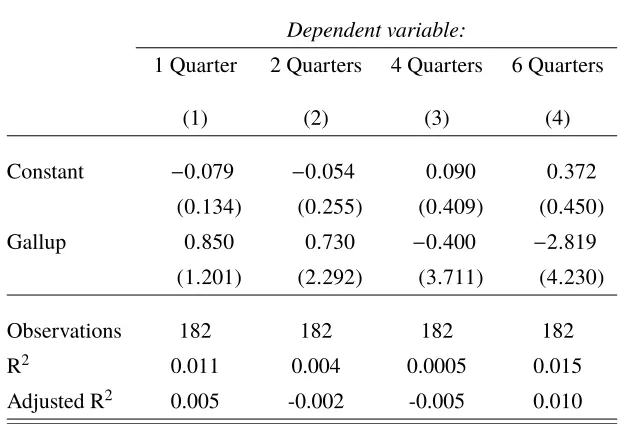
The documented patterns in Observations 1 and 2 provide evidence on the dynamics of investor beliefs. However, investor beliefs alone could not provide an answer to the question of how belief-based investor sentiment influences the market: as shown in Table A.3, Gallup survey measurement of investor sentiment doesnothave sig-nificant predictive power for future stock market returns. This result seems puzzling at the first glance since previous studies have shown that the extrapolation pattern in surveys reflect market-wide investor expectations—intuitively, the predictive pattern should be strong. One important element that seems missing is the wealth level of extrapolators: after all, extrapolators with extreme sentiment levels but with trivial wealth will have a limited impact on asset dynamics. Therefore, I also examine the wealth level of extrapolators.
To measure the wealth level of extrapolators, it is important to understand which group of investors are more susceptible to extrapolation. In the finance literature, a common way to categorize investors is to divide them into individual investors and institutional investors. Moreover, in the literature, individual investors are often believed to be less sophisticated and more vulnerable to psychological biases, a term formally defined as “dumb money” effect. And empirical evidence is prevailing. For instance, Odean (1999), Barber and Odean (2000) and Barber and Odean (2001) present extensive evidence that individual investors suffer from biased-self attribution, and tend to have wealth-destroying excessive trading. Frazzini and Lamont (2008) use mutual fund flows as a measure of individual investor sentiment for different stocks and find that high sentiment predicts low future returns.9
A reasonable proxy for individual investors exists in the Federal Reserve’s Z.1 Sta-tistical Release (“Financials Accounts of the United States”), which reports balance sheet information for different sectors of the economy at a quarterly frequency, in-cluding the Households and Nonprofit Organizations Sector (HNPO sector). The HNPO sector contains aggregated information about individual investors.
More importantly, as shown in the recent studies, individual investors in the HNPO sector tend to extrapolate. For example, a rigorous examination is reported in Yang
and Zhang (2017). Specifically, they document that (1) when investor expectations in the surveys are high, investors in the HNPO sector tend to increase their investment in the stock market; and (2) their investment choices negatively predict future stock market returns. These results together show that investors in the HNPO sector can serve as a reasonable proxies for extrapolators. Moreover, in my empirical analysis, I use the total financial wealth to proxy for the wealth level of extrapolators.10
Interaction Effect between Investor Sentiment and Wealth Level
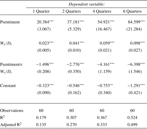
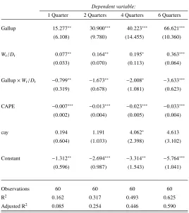
Investor sentiment should impact market strongly especially when the wealth level of extrapolators is high. In other words, there should be a strong interaction effect between investor sentiment and the wealth level of extrapolators in explaining asset valuations. To formally test this hypothesis and to motivate my model setting, I run the following regression11:
Rte+N = a+bSentt+cWt/Dt+dSentt ×Wt/Dt+t. (1.4)
In my regression, Rte+N represents the excess returns of the aggregate stock market during the future N months. In addition, I use investor sentiment in the Gallup survey and Psentiment, respectively, to proxy for Sentt, investor sentiment, and use
the total financial assets of HNPO sector at time t as the empirical proxy for the wealth levelWt. SinceWtis non-stationary, I get the series of real dividendDtfrom
Shiller’s website and get the normalized wealth level ofWt/Dt. My sample is at a
quarterly frequency and spans from 1996:12 - 2011: 9.12 For robustness check, I report predictive regressions over one to six quarters.
[Place Table A.4 about here]
The results reported in Table A.4 not only confirm the strong interaction effect between investor sentiment and the wealth level in determining the asset prices, but also point to the usefulness in explaining asset mispricings—the strong nega-tive coefficient for the interaction term indicates investor sentiment leads to asset overvaluations and undervaluations when the wealth level is high. When investor
10As long as the HNPO sector captures the general properties of extrapolators, it will help understand the impact of investor sentiment on the market.
11Alternatively, the market impact of extrapolators can be measured by the relative wealth of extrapolators compared to the price level of the risky asset. The regressions based on this intuition is reported in appendix A.5. The results remains robust.
sentiment is high, the market is highly overvalued due to the high irrational demand from extrapolators and therefore future returns are low; if investor sentiment is low, the future returns are high since the market is undervalued. In addition, compared to the univariate regression using investor sentiment variable, the conditional pre-dictability model has a significantly higher adjusted-R2. For instance, at the annual horizon, the goodness of fit for the predictive regression using investor sentiment alone is around 0.010, which is small compared to 0.039 in the conditional predictive regression. The increased adjusted-R2 supports the importance of the interaction effect in explaining the market mispricing. Therefore, I get the following observa-tion:
Observation 3. Investor sentiment strongly connects with market mispricing through the market impact of extrapolators.
Observation 3 provides strong evidence for the relation between the market mispric-ing, investor sentiment and the wealth level of extrapolators. Therefore, for a model that focuses on the impact of investor sentiment and market mispricing, the wealth level of extrapolators should also be incorporated.
1.3 The Behavioral Model
In this section, I build a behavioral model that focuses on the investor sentiment of extrapolators. Specifically, following the patterns of investor sentiment documented in section 1.2, I introduce extrapolation into my model. With extrapolation, the behavioral model essentially captures the overvaluations and undervaluations in the market and shed light on the time-varying impact of investor sentiment on the equilibrium asset price.
The Economy
I consider a continuous-time economy with two types of assets: one risk-free asset with elastic supply curve and a constant rater, and one risky asset with a fixed per-capita supply of one. Due to extrapolation, extrapolators perceive a biased growth rate of the risky asset, which is different from the true growth rate observed by the outside econometricians.
The risky asset is a claim to the underlying dividend processDtwhich, under the true
written as
dDt/Dt = gDdt+σDdωt. (1.5)
Therefore, the underlying dividend process is governed by the growth rate ofgDand
volatilityσD, which both are positive exogenous parameters. The dividend process is
driven byωt, a one-dimensional Weiner process under the true probability measure
observed by outside econometricians. The equilibrium price Pt for the dividend
claim evolves as
dPt/Pt = gP,tdt+σP,tdωt. (1.6)
Due to extrapolation, the true growth rategP,tis different from the perceived growth
rate by extrapolators. The growth rategP,t and volatility termσP,tare both
endoge-nously determined in the equilibrium.
Investors
There are two types of investors in the behavioral model: extrapolators and funda-mental investors. Extrapolators are the focus of this paper: their belief formation are subject to psychological heuristics and therefore are misspecified. Fundamental investors, on the other end, serves as the counteracting forces in the market and trade aggressively whenever asset prices deviate from fundamental values. Similarly, I assume that fundamental investors make up a fraction of 1− µand extrapolators make up a fraction of µ.
Extrapolative Beliefs
The salient properties about investor sentiment in the surveys—that investors form their expectations based on past realized returns and that their sentiment reverts quickly to its mean—motivate my theoretical settings for investor sentiment. Dif-ferent from asset pricing models with rational expectations, extrapolators in the behavioral model make systematic errors about future market returns. In order to capture the misspecified beliefs for investors, I propose a mental model.13 Specif-ically, I assume extrapolators perceive the following process for the market price, with the perceived growth rate ˆgP,t as an affine function of a latent state variable
St that essentially captures the excessive optimism and pessimism in extrapolators’
minds:
dPt/Pt =gˆP,tdt+σP,tdωte,
ˆ
gP,t ≡[(1−θ)g¯P,t+θSt]. (1.7)
Here ¯gP,t represents the equilibrium growth rate of risky asset in a benchmark
economy where each investors have correct beliefs. Parameterθmeasures to which extent extrapolators deviate from their beliefs in the rational benchmark. When
θ = 0, I get the rational benchmark case with a drift term ˆgP,t.14 Notation-wise,
any quantities with a hat sign or superscript e represent variables perceived by extrapolators.
Next, I introduce microfoundations for this key latent state variableSt. Specifically, I
assume that from the extrapolators’ perspective, the expected growth rate on the risky asset is an affine function of a mental variable ˜µP,t, and the extrapolators mistakenly
believe that this mental variable is governed by a regime-switching process between high and low states µH and µL, with switching densities χandλ:
*
, ˜
µP,t+dt = µH µ˜P,t+dt = µL
˜
µP,t = µH 1− χdt χdt
˜
µP,t = µL λdt 1−λdt
+
-. (1.8)
Motivated by the fact that investors in the survey over-extrapolate past returns when forming their expectations, I assume that extrapolators in my model update their estimate of the mental variable ˜µP,t by looking at the past realized returns.
Therefore, µH andµLreflect extrapolators’ subjective perceptions on the risky asset
growth rate, andλand χrepresent the speed extrapolators update their perceptions on the risky asset growth rate based on past realized returns. Given this mental model, the latent state variable St is the Bayesian inference of the mental variable
˜
µS,t. Formally, I can write the latent state variable asSt ≡Ee[ ˜µP,t|Ft], whereFt is
the perceived probability measure based on the filtration of the price processPt. My
later examination on extrapolators’ belief structure helps me justify the magnitude of these belief parameters.
Therefore, in my model, investor sentiment corresponds to the perceived growth rate of extrapolators, ˆgP,t. Throughout my model, I assume that each extrapolator
is subject to the identical underlying mental model and the same degree of extrap-olation. In other words, latent state variableθ reflects theconsensusextrapolation
14For a detailed solution for ˆg
level among extrapolators.
By applying the optimal filtering theorem (Liptser and Shiryaev (2013)), I obtain the dynamics for the latent state variableSt:
dSt = µSdt+σSdωte, (1.9)
where
µS=λ µH + χµL −(χ+λ)St, (1.10)
σS=σ−P,1tθ(µH −St)(St− µL), (1.11)
dωte=dPt Pt
−[(1−θ)g¯P,t+θSt]dt. (1.12)
This mental model captures two salient features of investor sentiment in the surveys. First, under the mental model, the latent state variable St is driven by the perceived
Brownian shockdωte, which strongly depends on the past realized returns. Increases in past realized returns dPt
Pt push up the perceived Brownian shock, which further
increases the latent state variableSt and the perceived growth rate of the risky asset
ˆ
gP,t. Therefore, the mental model naturally leads to an extrapolation pattern: high
returns in the past push up investor sentiment and low past returns make extrapolators pessimistic.
Second, the mental model embodies the fact that investor sentiment tends to revert to its mean. When the latent state variable is high, extrapolators mistakenly perceive a high level of growth rate for the risky asset. However, the objective probability measure remain unchanged. Unless extremely good shocks arrive, they will be constantly disappointed by the perceived Brownian shocksdωte in the future. As a result, the latent variable will quickly revert downwards. Similarly, if the latent state variable is low and extrapolators perceive a low level of growth rate, extrapolators will meet with relatively large perceived Brownian shocks, pushing up the latent state variable back to its mean.
en-dogenous reversal pattern in investor beliefs helps understand asset mispricings and predictability of returns generated in this model.15
Moreover, due to the mental model, the perceived probability measure by extrapola-tors is different from the objective probability measure observed by outside econo-metricians.16 In other words, extrapolators have misspecified but self-consistent beliefs, and they fail to realize that their perception is biased. The true and per-ceived probability measure can be connected using the following equation:
dωte = (gP,t−gˆP,t)/σP,tdt+dωt. (1.13)
Under the probability measure of extrapolators, the perceived dividend process follows
dDt/Dt =gˆD,tdt+σDdωte. (1.14)
where ˆgD,t is the perceived dividend growth rate by extrapolators.
In my model, gP,t, ˆgP,t and ˆgD,t are endogenous variables determined in the
equi-librium. As a comparison, the volatility variablesσP,t andσD remain unchanged.
This is because extrapolators can always calculate the volatilities by calculating the quadratic variations of the stochastic process. All the quantities together constitute two mutually coherent probability measurements.
Finally, it is worth pointing out that, there is a two-way feedback loop in my model: asset prices influence investor expectations due to extrapolation, and changes in investor expectation will in turn drive asset prices. From a theoretical perspective, a model with extrapolation on past returns is usually difficult to solve, since the return process is an endogenous quantity determined in the equilibrium. In this paper, I overcome this difficulty by solving a system of partial differential equations.
Wealth Process of Extrapolators
To better connect with later analyses on the time-varying impact of investor senti-ment, I introduce logarithmic utilities for extrapolators to capture the dependence of demand on their wealth level. Moreover, each extrapolator, indexed by superscript
15The pattern that investors tend to overweight recent information has been incorporated in other models as well. For instance, Bordalo et al. (2018) focus on investors’ belief formation of credit spreads, and proposed a mechanism in which investors overreact to recent news.
j, is infinitesimal and therefore acts as price-taker in the market. Specifically, ex-trapolator jmaximizes an additively separable logarithmic utility function under an infinite time horizon and with a time-preference parameter ρ
max
{Ctj+s}s≥0
Eet[
Z ∞
t
e−ρslnCsjds] (1.15)
subject to
dWtj =−Ctjdt+rWtjdt+αtjWtj[ ˆgP,tdt+
Dt
Pt
dt−r dt +σP,tdωet], (1.16)
whereWtj represents the wealth level of extrapolators,Ctj the optimal consumption choice and αtj the optimal risk exposure for extrapolator j. Ete represents the expectation operator under the perceived probability measure, which is biased due to extrapolation.
With the logarithmic utility, extrapolators have wealth-dependent absolute risk aver-sion: as their wealth declines to zero, extrapolators become infinitely risk-averse. Consequently, as their wealth shrinks, they will liquid the risky asset to prevent their wealth from becoming zero.17 In addition, the infinitely risk-aversion level at zero wealth level also prevents extrapolators from bankruptcy. Therefore, they can borrow money at risk-free rate irrespective of their wealth level.
Following the standard Merton’s approach (Merton (1971)), we get the optimal consumption and portfolio rule for extrapolators:
PROPOSITION 1 Extrapolators with the objective function in equation (1.15) and wealth process in equation (1.16) will optimally consume and invest at timet
according to the following strategies:
Ctj = ρWtj (1.17)
and
αj
t =
ˆ
gP,t(xt,St)+l−1(xt,St)−r
σ2
P,t(xt,St)
, (1.18)
where the price to dividend ratio l ≡ Pt
Dt and the risky asset volatility σP,t both
depend on the wealth to dividend ratio xt ≡ WDtt and the latent state variable St. In other words, the economy depends on state variablesxt andSt.
Proof: See Appendix A.3.
Proposition (1) documents several salient features of logarithmic utilities. First, the optimal consumption strategy for extrapolators is proportional to their wealth level, with adjustment of the time-preference parameters ρ. Second, the optimal risky portfolio choice is myopic, in a sense that extrapolators do not hedge against changes in the future investment set. Therefore, their optimal risky exposure purely depends on the perceived risk premium and the instantaneous volatility rate. Third, the total dollar demand is also proportional to their wealth. Therefore, their wealth level, by and large, determines their market impact on the equilibrium asset prices—a key property that drives my model implications.
In the equilibrium, the risky exposure of extrapolators depends on their perceptions of equity premium, ˆgP,t + l−1 −r. After observing a sequence of high (low)
re-turns, extrapolators become overly optimistic (pessimistic) and increase their risky asset exposure. In cases when their market impact is high, asset tends to become overvalued (undervalued).
More importantly, the optimal strategy in equation (1.18) and the wealth dynamics in equation (1.16) together provide novel insights on how investor sentiment influences the wealth dynamics of extrapolators. When investor sentiment is high, extrapolators perceive high equity premium and therefore lever up to buy risky asset. However, since investor sentiment reverts to its mean, extrapolators demand less risky asset in the future, which leads to decreases in the asset prices and their wealth level, therefore generating negative returns. In the mean-reversion process, the wealth dynamics of extrapolators also play a role: investor sentiment leads investors to take excessive exposure to the risky asset and therefore suffer from wealth decrease. Decline in the wealth level of extrapolators makes the mispricing easier to correct.
Fundamental Investors
this assumption, the per capita demand of the risky asset for fundamental investors follows
Qt = (PF,t− Pt)/k, (1.19)
wherePF,t = r−DgtD is the fundamental value andk is a constant. This linear demand
structure is standard in the literature (for example Xiong (2001)), and I provide a micro-foundation for it in the appendix A.1. Intuitively, whenPF,tis higher (lower)
than its current price, fundamental investors expect profits when asset prices reverts back to the fundamental value Pt. Therefore, they have a strong demand to short
(buy) the risky asset.
Fundamental investors are prevailing in the financial market. There are many in-vestors who truly follow strategies that focus on the long-term profit and apply fun-damental analysis in their investment. For instance, Abarbanell and Bushee (1997) document that investors incorporate financial statement information and make fun-damental analysis when making their investment decision. In addition, there are many mutual funds who set their investment objective as to achieve long-term growth of capital and income, such as the “Fundamental Investor” fund managed by Capi-tal Group. Moreover, such fundamenCapi-tal analysis really brings abnormal returns to their portfolio. For instance, Piotroski (2000) document fundamental analysis can increase annual returns by at least 7.5%.
Several observations about the total dollar demand in equation (1.19) are worth noting. First, for fundamental investors, the total dollar demand is independent of their wealth level, rather, it only depends on the difference between the current risky asset prices and their fundamental values. When asset prices are highly overvalued, fundamental investors anticipate a higher return from holding the risky asset and, as a result, their total dollar demand increases. Conversely, when asset prices are undervalued, fundamental investors lean against the wind and trade actively to push prices upward. Moreover, the extent to which fundamental investors can correct the mispricing also depends on the overall market impact of the extrapolators: if the wealth level of extrapolators is low, fundamental investors can correct mispricing more easily. This demand structure of fundamental investors proves to be useful in generating novel implications on the predictive pattern of investor sentiment.
have a specific demand function due to unspecified factors such as financial frictions or preference shocks.
Equilibrium
Definition of Equilibrium:
An equilibrium in the behavioral model satisfies the following conditions:
i) extrapolators maximize their objective function in equation (1.15) subject to their wealth process in equation (1.16) under their subjective probability measure induced by extrapolation;
ii) fundamental investors invest in the risky asset according to their demand function in equation (1.18);
iii) risky asset market clears
µαtWt+(1− µ)Qt = Pt. (1.20)
To solve for the equilibrium, I face with a fixed-point problem: the optimal demand of extrapolators depends on the instantaneous equity premium and volatilities of the risky asset, which further depends on the total demand in the equilibrium. For the behavioral model, I focus on the symmetric equilibrium where each extrapolator endows with the same level of wealth and follows identical strategies and solve for a fixed-point problem. The equilibrium depends both on the wealth to dividend ratio
xt and the latent state variableSt. Therefore, I rely on solving a partial differential
equation to obtain the solution for the fixed-point problem. As verified later, the price to dividend ratio is monotonically increasing in both xt andSt.
After getting the optimal strategy for extrapolators, now I consider a fixed-point problem and solve the Markovian system to get an solution of the price-dividend ratiol(St,xt). To be specific, I focus on an equilibrium, where each extrapolator j
follows the same strategies based on the return extrapolation. By using aggregation and the market clearing condition, I can reach the equilibrium as follows:
PROPOSITION 2 In the symmetric equilibrium, the price-dividend ratio l is a function of current states St and xt, and satisfies the following partial differential equation:
c0l−c1
x =
ˆ
gP,t+l−1−r
σ2
P,t
whereσPis also a function of St andxt and satisfies
σP,t = (lx
l x−1)σD − q
(lx
l x−1)2σ
2
D −4(
lx
l (c0l−c1)−1) lS
l θ(µH −S)(S− µL)
2(lx
l (c0l−c1)−1)
,
(1.22)
andl(St,xt) satisfies the following boundary conditions
lim
xt→0
l = c1 c0
, (1.23)
lim
xt→0
= lim
x→0 ˆ gP,t+ cc1
0 −r
σ2
D
, (1.24)
and
lim
xt→∞
l = (r −gˆP,t)−1, (1.25)
wherec0=
k+1−µ
kµ andc1 =
1−µ
kµ(r−gD) are both constants.
In addition, under the perceived probability measure, the dynamics of xt follow
dxt =gˆx,t(St,xt)dt+σx,t(St,xt)dωet, (1.26)
where
ˆ
gx,t(St,xt) =xt(r− ρ+αt[ ˆgP,t +l−1−r]−gˆD,t +σ2D −αtσDσP,t) (1.27)
σx,t(St,xt) =xt(αtσP,t−σD).
Proof: See Appendix A.3.
For the boundary conditions, when the wealth to dividend ratio goes to zero, the fundamental investors dominate the market and I get a constant price-dividend ratio in equation (1.23). Moreover, in this case, the partial derivative oflwith respect to
S,lS(S,0), equals to zero because extrapolators’ total demand is zero irrespective of the level of the latent state variableSt. On the other hand, whenxtgoes to infinity, in
order to clear the market, extrapolators hold a risky asset position close to zero. By the portfolio expression in equation (1.18), we get the expression (1.25). Expression (1.24) follows naturally from equation (1.23).
of [0,∞], the required domain for Chebyshev polynomial is [−1,1]. Therefore, I apply the following monotonic transformation for the wealth to dividend ratio
zt =
xt−ξ
xt+ξ
, (1.28)
whereξis a positive constant. Along with the transformed wealth to dividend ratio, I also transform the latent state variable S into a new variable y that lies between [−1,1]:
yt =aSt+b, (1.29)
a = 2
µH − µL
, b=−µH +µL
µH −µL
.
When the wealth to dividend ratio goes to infinity, the transformed wealth to dividend ratio goes to 1. If the wealth to dividend ratio shrinks to zero, the transformed wealth to dividend ratio goes to−1. Similarly,ytgoes to 1 whenStgoes to its upper bound
µH, and goes to -1 when St goes to its lower bound µL.
Calibrated Model Solution
In this section, I report the main numerical solutions. To get a reasonable model solution, I choose both asset and utility parameters that are consistent with the empirical literature. For example, I set gD to be 1.5% andσD to be 10%, which
are commonly used in the asset pricing literature. In addition, I setr = 4% for the risk-free rate. For utility parameters, I choose the time-preference factor ρ = 2%. For other parameters that have no empirical counterparts, such as µand k, I take a neutral stand and impose a value of 12. For belief parameters, I set µH = 0.03,
µL = −0.06, χ = λ = 10%, θ = 0.5%. A complete set of parameter values are
reported in Table A.6. I report the numerical solutions in Figure A.5.
Price-Dividend Ratio
The upper-left panel reports the price to dividend ratiol(St,xt). In general,l(St,xt)
is a monotone function both in the transformed wealth to dividend ratio zt and the
latent state variable yt. First, for most of zt levels, a higher latent variable level St
if extrapolators have no wealth, they will have no market impact on the equilibrium quantities. Second, with a fixed level of latent variable yt, the dollar demand for
the risky asset increases as zt increases. With given parameters, the solution for
l(St,xt)ranges from 20 to 35, which is largely within the reasonable range.
[Place Figure A.5 about here]
Optimal Portfolio Choice
I report the optimal portfolio choice for extrapolators in the lower-right panel. As yt increases along the axis, extrapolators perceive higher growth rate and therefore
increase their position in the risky asset. Asztincreases from−1 to 1, in general, the
optimal portfolio decreases in order to meet the market clearing condition. Together, I get the optimal strategies of extrapolators. It is worth noting that, when bothztand ytare low and extrapolators have low market impact and become pessimistic about
future return growth, they can short the risky asset; in other situations, extrapolators hold the risky asset.
Volatility
The upper-right panel portrays the return volatilityσP. In most of the cases,σP is
larger than σD. When the wealth to dividend ratio xt is high and the latent state
variable St is slightly above its mean, the volatility σP reaches its maximum of
17.78%.
Along the latent variable axis, the volatility has a strong hump-shaped pattern due to the belief structure. Specifically, when the latent variable yt goes to its upper or
lower boundary, there is less uncertainty about which regime the underlying state belongs to. On the contrary, when yt is in the middle region between the high and
low bound, the uncertainty increases.
Moreover, increases inztin general increases the market impact of extrapolators. As
a result, their beliefs have a stronger amplification effect on the exogenous shocks, which explains the increasing volatility along theztaxis. However, whenyt reaches
its maximum or minimum, the volatility is mainly determined by changes inztratio.
When yt is at its maximum, the optimal portfolio is positive but less than one. In
volatility.18 Conversely, when yt is at its minimum, the optimal portfolio is, by
and large, negative. In this case, extrapolators short the risky asset. When positive dividend shocks arrive, extrapolators’ leverage ratio further decreases and induces them to buy more risky assets, which increases the volatility.
Two Model Predictions
Investor Sentiment and Market Mispricing
In this model, I simultaneously characterize investor sentiment and the wealth level within one unified model, which provides novel insights between investor sentiment and market mispricing. From a static perspective, the market clearing condition in equation (1.20) helps to identify when the market overvaluations and undervalua-tions would occur. When the wealth level of extrapolators is high, investor sentiment has large impacts on the market: with high investor sentiment, the asset price is largely overvalued; while if investor sentiment is low, the asset price is undervalued.
Investor Sentiment and Return Predictability
The dynamic feature of the behavioral model also sheds light on the connection between investor sentiment and the future asset price dynamics. With higher wealth level, a larger fraction of total asset demand will come from extrapolators. Con-ditional on high wealth level, high investor sentiment will push asset prices above their fundamental value. However, higher sentiment will revert to its mean quickly, since optimistic investors will more easily get disappointed by the future realized returns. Consequently, both investor sentiment and asset prices will decline in the future, generating negative returns. Conversely, conditional on high wealth level, low investor sentiment predicts a high returns going forward. This together implies a strong negative pattern for investor sentiment when wealth level is high.
Moreover, my model implies a novel predictive pattern of investor sentiment on future returns when the wealth level of extrapolators is low. In this situation, asset prices are mainly driven by fundamental investors and the sentiment of extrapola-tors reflects the direction of market correction. If extrapolaextrapola-tors have high sentiment, extrapolation indicates that the recent returns in the past were high and the mar-ket is undergoing an upward correction. Therefore, high sentiment implies good future returns along this upward path. Conversely, if extrapolators have low
timent, extrapolation indicates a downward correction, and fundamental investors will continue shorting risky asset until asset price reaches its fundamental value. Low sentiment predicts negative returns along this path. Together, conditional on the low wealth level of extrapolators, investor sentiment positively predicts future market returns.
Figure A.3 provides intuitive explanations for the positive predictive pattern of investor sentiment when the wealth level of extrapolators is low. If investor sentiment is low, extrapolation indicate that the asset price is undergoing a upward correction. Therefore, the only possible price dynamics is the one that goes up but is below the fundamental value—the wealth level of extrapolators is too low to push asset prices upwards from the fundamental value. Conversely, if investor sentiment is low, then the only possible situation is that the asset price is corrected downwards from overvaluations—the low market impact of extrapolators is not able to push asset prices downwards from the fundamental value.
[Place Figure A.3 about here]
1.4 Model Implications
In this section, I provide analyses for the behavioral model based on simulations. Specifically, I start by checking the belief pattern of extrapolators to see whether it captures the investor sentiment dynamics in the survey. Then I test whether there is a strong connection between investor sentiment and market mispricing, and test the key model implications on the return predictability based on investor sentiment. I also use my model to shed some light on the extant asset pricing patterns in the empirical literature.
Extrapolators’ Beliefs
to the literature. Last, I test whether the model-implied investor sentiment reverts to its mean.
To simulate my model, I back out a sequence of shocks based on the monthly real dividend data of the S&P 500 index starting from June 1996 to December 2011. This range is consistent with the Gallup series in Greenwood and Shleifer (2014) and therefore can facilitate my comparison between the simulated sentiment series and the survey data. Moreover, I also use these implied shocks for my analyses of the behavioral model, so that I can compare two models within the same background.
Specifically, in order to get the series of shocks, I take the log on the dividend process and then use Ito’s lemma to get
dlnDt = (gD−
1 2σ
2
D)dt+σDdωt. (1.30)
Then, I can discretize the equation and back out the shocks using the following formula:
t = (lnDt+1−lnDt−(gD −
1 2σ
2
D)∆t)/(σD p
∆t). (1.31)
Since the real dividend data is at a monthly frequency, I set ∆t equals to 1/12. In
addition, I set gD as 1.5% and σD as 10%, which are both commonly accepted
magnitudes in the asset pricing literature. I take a neutral stand and set the initial sentiment level to be S0 = 0. I also set the initial wealth to dividend ratio x0 to be 1. Since I have numerically solved the equilibrium, I can easily get the simulated sequence for investor sentimentSt, price processPt, the wealth-dividend
ratio process xt as well asl(St,xt),gP,t(St,xt)andσP(St,xt).
Model-implied Investor Sentiment
[Place Figure A.6 about here]
Extrapolative Belief Structures
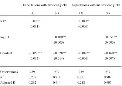
Next, I zoom in the extrapolation pattern in my behavioral model. Greenwood and Shleifer (2014) documents that investor expectations about future returns heavily depend on the current price level and past realized returns. Specifically, I regress the perceived expectations of future returns on either the current log price-dividend ratio or the past twelve-month accumulative raw returns, based on the simulated series. I report the regression coefficients, their t-statistics and their R-squared in Table A.7. For robustness check, I report results based on two different types of expectation measures: the expectations of future return growth ratedPt/(Ptdt)and
the expectations of future return growth rate with dividend yielddPt/(Ptdt)+l−1.
Table A.7 indicates the investor belief pattern in my model matches the extrapolation pattern documented in Greenwood and Shleifer (2014). Among others, both in my model and in the survey, subjective expectations on future returns are positively related to the current log price-dividend ratio and the past twelve-month returns. Moreover, the regression coefficients and t-statistics are also close to the regression results based on the Gallup survey. For instance, compared to the regression coeffi-cient of 9.12% and t-statistics of 8.81 from regressions based on Gallup survey, my simulation-based regression yields coefficient of 2.3% and t-statistics of 2.09.
[Place Table A.7 about here]
Extrapolators’ Memory Span
Another important dimension of investor belief structure is its memory span, which measures how much weight extrapolators put on the recent returns. In my model, extrapolators’ memory span is controlled by the magnitude of belief parameters χ andλ, which determines how fast extrapolators update their beliefs. To formally test extrapolators’ memory span, I run the nonlinear regression following Greenwood and Shleifer (2014):
Expectationt =a+bΣ∞s=0ωsRt−(s+1)∆t,t−s∆t, (1.32)
ωs =
e−ψs∆t
In Table A.8, I report the regression coefficienta, the interceptb, the adjusted-R2, and more importantly, the estimated memory span parameterψ. My simulation is at monthly frequency and therefore I set∆=1/12. I imposen= 600, which means