The Plane Waves Method for Numerical Boundary Identification

Identification

.

White Rose Research Online URL for this paper:

http://eprints.whiterose.ac.uk/114571/

Version: Accepted Version

Article:

Karageorghis, A, Lesnic, D and Marin, L (2017) The Plane Waves Method for Numerical

Boundary Identification. Advances in Applied Mathematics and Mechanics, 9 (6). pp.

1312-1329. ISSN 2070-0733

https://doi.org/10.4208/aamm.OA-2016-0185

© Global-Science Press 2017 . This is an author produced version of a paper published in

Advances in Applied Mathematics and Mechanics. This version is free to view and

download for private research and study only. Not for re-distribution, re-sale or use in

derivative works. Uploaded in accordance with the publisher's self-archiving policy.

[email protected] https://eprints.whiterose.ac.uk/ Reuse

Items deposited in White Rose Research Online are protected by copyright, with all rights reserved unless indicated otherwise. They may be downloaded and/or printed for private study, or other acts as permitted by national copyright laws. The publisher or other rights holders may allow further reproduction and re-use of the full text version. This is indicated by the licence information on the White Rose Research Online record for the item.

Takedown

If you consider content in White Rose Research Online to be in breach of UK law, please notify us by

A. KARAGEORGHIS, D. LESNIC, AND L. MARIN

Abstract. We study the numerical identification of an unknown portion of the boundary on which either the Dirichlet or the Neumann condition is provided from the knowledge of Cauchy data on the remaining, accessible and known part of the boundary of a two-dimensional domain, for problems governed by Helmholtz-type equations. This inverse geometric problem is solved using the plane waves method (PWM) in conjunction with the Tikhonov regularization method. The value for the regularization parameter is chosen according to Hansen’s L-curve criterion. The stability, convergence, accuracy and efficiency of the proposed method are investigated by considering several examples.

1. Introduction

The Helmholtz and modified Helmholtz equations are related to various physical applications in science and engi-neering. More specifically, these equations are used to describe the Debye-Hückel equation [15], the scattering of a wave [17], the linearization of the Boltzmann equation [35], the vibration of a structure [6], the acoustic cavity problem [12], the radiation wave [19] and the steady-state heat conduction in fins [33]. In general, we assume the knowledge of the geometry of the domain of interest, the boundary conditions on the entire boundary of the solu-tion domain and the so-called wave parameter,κ, and this gives rise todirect/forward problemsfor Helmholtz-type equations, which have been extensively studied both mathematically and numerically, e.g. [24, 34]. When one or more of the above conditions for solving the direct problem associated with Helmholtz-type equations are partially or entirely unknown, then an inverse problem may be formulated to determine the unknowns from additional responses.

Traditional numerical methods, in conjunction with an appropriately chosen regularization/stabilization method, have been employed to solve inverse problems associated with Helmholtz-type equations, such as the finite-difference method (FDM) [4, 5], the finite element method (FEM) [25, 26] and the boundary element method (BEM) [39, 40], respectively. Both the FDM and the FEM require the discretization of the domain of interest which is time consuming and tedious, especially for complicated geometries. On the other hand, while the BEM is a boundary discretization method and hence reduces the dimensionality of the problem by one, however it requires the evaluation of singular integrals involving the fundamental solution and its normal derivative and the corresponding BEM matrices are fully populated.

An alternative to these traditional numerical methods are the so-called meshless methods which have been used extensively in the last two decades for retrieving accurate, stable and convergent numerical solutions to inverse problems for Helmholtz-type equations. The advantages of meshless methods are the ease with which they can be implemented, in particular for problems in complex geometries, their low computational cost and the fact that, in general, they are exempted from integrations that may become cumbersome, especially in three dimensions. Such methods include the boundary particle method (BPM) [13], the singular boundary method (SBM) [14], the method of fundamental solutions (MFS) [16], the boundary knot method (BKM) [23], Kansa’s method [28], etc.

Date: April 5, 2017.

2000Mathematics Subject Classification. Primary 65N35; Secondary 65N21, 65N38.

Key words and phrases. plane waves method, collocation, inverse problem, regularization.

The plane waves method (PWM) is a meshless Trefftz method applicable to the solution of boundary value problems governed by the Helmholtz or modified Helmholtz equation, [1, 2, 44], see also [20, Section 11.1.3]. The PWM has since been applied to the modified Helmholtz equation in [36], for the calculation of the eigenfrequencies of the Laplace operator in [3] and for the solution of inverse problems of Cauchy type in [22]. More recently, it was applied to the solution of direct axisymmetric Helmholtz problems in [29].

The PWM is closely related to another meshless Trefftz method, the method of fundamental solutions (MFS) [16] which has in recent years become very popular for the solution of inverse problems [31, 32]. The reason for this popularity is due to the fact that it is meshless and of boundary type, hence the MFS is easy to implement for problems in complex geometries in two and three dimensions. These properties are shared by the PWM which was shown to be an asymptotic version of the MFS in [2]. Moreover, the PWM has a considerable advantage over the MFS as it does not require an external pseudo-boundary on which the sources are to be placed. The location of this pseudo-boundary has been a major issue in the application of the MFS [11].

The PWM has apparently never been applied toinverse geometric problems[32] and in this study we investigate its application to a particular class of such inverse problems, namelyboundary identification problems. For Helmholtz-type equations such problems have been solved using the BEM in [37] and the MFS in [7, 38]. The paper is organized as follows. In Section 2 we present the inverse geometric problem under investigation. The numerical method employed for the approximate solution of the problem, namely the PWM, and the Tikhonov regularization method are described in Section 3. Five examples are considered and thoroughly investigated in Section 4. Finally, some concluding remarks and ideas for future work are presented in Section 5.

2. The problem

We consider the inverse geometric boundary value problem given by

∆u+κ2

u = 0 in Ω, (2.1a)

whereκ∈C∗ _{is given, subject to the Cauchy boundary conditions}

u = g1 and ∂u

∂n = g2 on ∂Ω1, (2.1b)

and the Robin boundary condition

αu+β∂u

∂n = g3 on ∂Ω2, (2.1c)

whereΩis a simply-connected bounded domain inR2 _{with smooth or piecewise smooth boundary∂Ωpartitioned}

into two disjoint parts ∂Ω1 (known) and ∂Ω2 (unknown), andg1, g2, g3 are given functions. In (2.1b) and (2.1c), ∂/∂nis the partial derivative along the outward normal unit vector n = (nx, ny)to the boundary at the point

(x, y), andαandβ are given coefficients satisfyingαβ≥0. A Dirichlet or Neumann boundary condition in (2.1c) is obtained if α= 1, β = 0or α= 0, β = 1, respectively. Ifκis real and positive representing the wave number, then equation (2.1a) becomes the Helmholtz equation in acoustic scattering, whilst ifκ= iλwith i = √−1 and

λreal and positive representing a heat transfer coefficient, then equation (2.1a) becomes the modified Helmholtz equation governing heat conduction in fins.

In problem (2.1a)-(2.1c) the goal is to determine uas well as the boundary ∂Ω2. This portion of the boundary

is presumed damaged due to a possible corrosion attack and the corrosion coefficient γ :=β/α is also known as the impedance coefficient. Physically, in general we have that in (2.1c), g3 = 0. Uniqueness of solution (u, ∂Ω2)

satisfying (2.1a), (2.1b) and (2.1c) holds [21] in the case of a perfectly conducting boundary(α= 1, β= 0, g3= 0) on which

or an insulated boundary(α= 0, β= 1, g3= 0)on which

∂u

∂n = 0 on ∂Ω2, (2.1e)

provided thatg2̸≡0(org1̸≡constant). In the case of a homogeneous Robin boundary condition

u+γ∂u

∂n = 0 on ∂Ω2, (2.1f)

there exist counterexamples, [7], for which uniqueness of solution fails.

Prior to this paper, the inverse geometric problem (2.1a)-(2.1c) has been solved using the BEM in [37] and the MFS in [38], and it is the purpose of this study to develop the PWM for solving the same problem. In addition, we make a comparison between the MFS and the PWM and also investigate a physical example withg3= 0.

3. The plane waves method

In the PWM [2], we approximate the solution uof boundary value problem (2.1a)-(2.1c) by a linear combination of plane waves

uL(x) = L ∑

ℓ=1 aℓeiκ

x_·dℓ

, x= (x, y)∈Ω. (3.1)

The justification of the PWM approximation (3.1) is based on the fact that the span of the set of plane wave functions {

eiκx_·d d=

(

cosφ,sinφ)

, φ∈[0,2π)}

is dense, in the L2

(Ω)-norm, in the set of functions satisfying equation (2.1a), [10]. In (3.1), the vectors dℓ are unitary direction vectors with distinct directions and, clearly,

each plane wave in the above expansion satisfies the Helmholtz equation (2.1a). As a result, in order to determine the unknown complex coefficients {aℓ}L_ℓ=1 we only need to satisfy the boundary conditions of the boundary value

problem in question, in our case (2.1b) and (2.1c). Density results regarding approximation (3.1) may be found in [2] where it is also shown that the PWM may be viewed as an asymptotic version of the MFS.

In the PWM we select M + 1 uniformly distributed boundary collocation points on ∂Ω1 and N −1 uniformly

distributed boundary collocation points on ∂Ω2. In particular, if the domain Ω = {(r(ϑ), ϑ)|ϑ∈[0,2π)} is a

star-like domain, we choose the boundary points on∂Ω1 to be, in polar coordinates,

xm=rm(cosϑm,sinϑm), ϑm=

(m−1)π

M , m= 1, . . . , M+ 1, (3.2)

while the boundary collocation points on∂Ω2 are

xM+1+j =rM+1+j(cosθj,sinθj), θj =π+ jπ

N, j= 1, . . . , N−1, (3.3)

where

rm=r(ϑm), m= 1, . . . , M+ 1, (3.4a)

and

rM+1+j =r(θj), j= 1, . . . , N−1, (3.4b)

Moreover, we choose theLunitary direction vectors to be

dℓ= (cosφℓ,sinφℓ), φℓ=

2(ℓ−1)π

L , ℓ= 1, . . . , L. (3.5)

Clearly, there could be other choices for theLunitary direction vectorsdℓ, ℓ= 1, . . . , L.The proposed choice given

3.1. Implementational details. In the PWM described above we have a total of2L+N−1unknowns consisting of the 2L unknown coefficients a ={aℓ=αℓ+ iβℓ}

L

ℓ=1, as well as the N−1 unknown positive radii values r =

{rM+1+n} N−1

n=1. These are determined by imposing the boundary conditions (2.1b) and (2.1c). By imposing

boundary conditions (2.1b) at the M+ 1 points (3.2) we obtain 4(M+ 1) equations (taking real and imaginary parts) and by imposing boundary condition (2.1c) at theN−1points (3.3) we obtain a further2(N−1)equations. Thus, the total number of equations is4M+ 2N+ 2and for a determined or over-determined situation we therefore need to have 4M +N ≥ 2L−3. The imposition of the boundary conditions (2.1b) and (2.1c) is achieved by minimizing the regularized non-linear least-squares functional

F(a,r) =

M+1 ∑

m=1

uL(xm)−g1(xm) 2 + M+1 ∑ m=1 ∂uL

∂n (xm)−g2(xm) 2 + N−1 ∑ j=1

αuL(xM+1+j) +β ∂uL

∂n (xM+1+j)−g3(xM+1+j) 2 +λ1 L ∑ ℓ=1

|aℓ|2+λ2 N−1

∑

j=2 (

rM+1+j−rM+1+j−1 )2

, (3.6)

whereλ1, λ2≥0are regularization parameters and| · |denotes the modulus of a complex number.

Remarks.

(i) The normal derivative flux data in (2.1b) comes from practical measurement which is inherently contaminated with noisy errors, and therefore we replaceg2 bygϵ

2 given by

gϵ

2(xm) = (1 +ρmp)g2(xm), m= 1,(M+ 1), (3.7)

where prepresents the percentage of noise andρj is a pseudo-random noisy variable drawn from a uniform

distribution in[−1,1]using the MATLAB⃝c _{command-1+2*rand(1,M+1).} (ii) In (3.6), the outward normal vectornis defined as follows:

n(ϑ) = √ 1 r2_{(ϑ) +r}′2

(ϑ)

[(r′_{(ϑ) sinϑ+r(ϑ) cosϑ)i−(r}′_{(ϑ) cosϑ−r(ϑ) sinϑ)j], (3.8)}

wherei= (1,0) andj= (0,1). In (3.8), we use the finite-difference approximation

r′_(ϑ i)≈

ri+1−ri−1

2π/N , i=M + 2, M+N , (3.9)

with the convention thatrM+N+1=r1.

(iii) The last term in (3.6) imposes aC1_{-smoothness constraint on the unknown boundary∂Ω}

2. In previous studies,

[8, 30], we imposed a C0_{-continuity constraint for similar shape detection problems, but, after extensive}

experimentation, found that the results with the higher-order C1_{-smoothness are more accurate. Of course,}

to impose the correct degree of smoothness requiresa priori knowledge about the regularity of the unknown boundary, e.g. if it is known that ∂Ω2 has corners, then a total variation constraint, [9], would be more

appropriate. Finally, it should be noted that in the absence of sucha priori information on the smoothness of the unknown boundary, one does not need to penalise it, but instead needs to stop the iteration process at an appropriate threshold. More details regarding general optimisation for nonlinear and ill-posed problems can be found in [27].

(iv) The minimization of functional (3.6) is carried out using the MATLAB⃝c _{optimization toolbox routine}

bounds on a but ris bounded between 0 and 1.2 (for Examples 1-5). Unless otherwise stated, we took the initial guess (a0,r0) = (0_,0_.5_).

(v) In the implementation of the method, we split the unknown coefficientsa={aℓ} L

ℓ=1 into real and imaginary

parts{aℓ=αℓ+ iβℓ}L_ℓ=1. Inlsqnonlin(which can only handle real variables) all the unknowns are real and

consist of the2Lreal and imaginary parts of the coefficients{αℓ} L

ℓ=1 and{βℓ} L

ℓ=1, respectively, and the radii

values r = {rM+1+n} N−1

n=1. For the imposition of the boundary conditions (2.1b) and (2.1c), the complex

approximation (3.1) is obtained from first constructing the complex coefficients{aℓ} L

ℓ=1 from their real and

imaginary parts. The boundary conditions (2.1b) and (2.1c) are imposed by imposing the satisfaction of both their real and the imaginary parts. Thus the functions provided tolsqnonlinare all real.

4. Numerical examples

In all figures presented in this section the reconstructed boundary is shown in red dots (· · ·). In numerical Examples 1 and 2 below we choseκ=√2and consider boundary datag1, g2andg3constructed from the analytical solution

u(x, y) = eax+by_{, (4.1)}

wherea= 0.1andb= i√a2_+κ2_.

4.1. Example 1. We first consider the unit disk Ω in which ∂Ω1 and ∂Ω2 are the upper and lower semicircle,

respectively, that is,

∂Ω1= {

x= (x, y)| −1≤x≤1;y=√1−x2} _(4.2a)

and

∂Ω2= {

x= (x, y)| −1≤x≤1;y=−√1−x2}_{. (4.2b)}

4.2. Example 2. We next consider a peanut-shaped domain described parametrically by

Ω ={

x= (x, y)|x2

+y2 < r2

(ϑ); ϑ∈[0,2π)}

, where r(ϑ) =

√

cos2_ϑ+1

4sin

2

ϑ (4.3)

and∂Ω1and∂Ω2 are defined by

∂Ω1={x= (x, y)|x=r(ϑ) cosϑ;y=r(ϑ) sinϑ, ϑ∈[0, π]}, (4.4a)

∂Ω2={x= (x, y)|x=r(ϑ) cosϑ;y=r(ϑ) sinϑ, ϑ∈(π,2π)}. (4.4b)

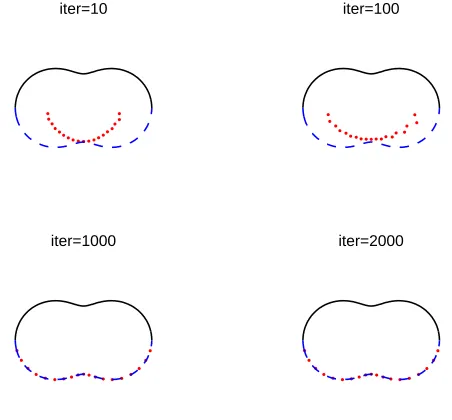
In Figures 1 and 3 we present some results with no noise and no regularization for α = 1, β = 0 (Dirichlet boundary condition on∂Ω2) and M = 10, N = 20, L= 20for various numbers of iterations, for Examples 1 and

2, respectively. The corresponding results for α= 0, β = 1(Neumann boundary condition on∂Ω2) are presented

in Figures 2 and 4. From Figures 1-4 it can be seen that in case of no noise the iterative reconstructions are convergent to the true shapes (4.2b) and (4.4b) for both Examples 1 and 2, respectively, and for both Dirichlet and Neumann problems in about 2000 iterations. It can be observed that for the Neumann problem convergence is reached after about 1000 iterations whilst for the Dirichlet problem convergence requires more iterations, i.e., the iterative method converges faster for the former problem than for the latter problem. An argument regarding the number of iterations will be presented in the next paragraph.

oscillations manifesting, especially near the points where the boundaries ∂Ω1 and ∂Ω2 meet. These oscillations

are likely to grow, as the number of iterations increases, due to the instability of the nonlinear ill-posed problem. In order to restore stability, regularization is employed. As stability is ensured through appropriate choices of the regularization parametersλ1and/orλ2, there is no need to cease the iteration process at a threshold dictated by a discrepancy-type stopping criterion. In this situation, the iterative process can be allowed to run until no further progress is realised and convergence has achieved a level of stationarity (in our case, in around 2000 iterations). The numerical reconstructions after 2000 iterations presented in Figures 6 and 7 show that regularization withλ1

retrieves very accurately the desired shape (4.4b) whilst regularization withλ2 has less of an effect. From Figure 7 one would probably choose a regularization parameter λ2 between10−2 _{and 10}−1_{, but from Figure 6 one can see}

that a wide range of values ofλ1between10−10 _and10−4 _{all produce stable and very accurate results.}

4.3. Example 3. We investigate an example considered in [38] given byκ= 1and

u(x, y) = cos

( x+y

√ 2

)

(4.5)

in the unit circle with ∂Ω1 and ∂Ω2 given by (4.2a) and (4.2b), respectively. We consider the Neumann case α= 0, β= 1. We tookM = 12, N = 12, L= 14with initial guess(a0_,r0_{) = (0,0.55)and examined the effect of}

regularization with noisep= 5%. Similar results have been obtained forp= 10%and are therefore not presented. The effects of regularization with λ1 or λ2, after 2000 iterations, are presented in Figures 8 and 9, respectively. From these figures, it can be seen that regularization withλ1between10−5

and10−3

, or withλ2between10−3

and 101

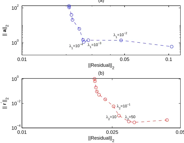
produces stable and accurate reconstructions of the semicircular shape (4.2b). In order to give a justification for the choice of the regularization parameters, the L-curves, see [18], are plotted in Figure 10. From this figure, it can be seen that L-shaped curves are indeed obtained when plotting, on a log-log scale, the residual (given by the square root of the first three terms in the right-hand side of (3.6)) versus the solution norm||a_|| or||r′_{||given by}

the square root of the fourth or fifth term, respectively, in the right-hand side of (3.6). Then, selecting values of

λ1or λ2near the corners of these L-curves provide suitable candidates for appropriate regularization parameters, balancing smoothing versus stability.

We finally mention that the results obtained with the PWM in Figures 8 and 9 are comparable to those in Figure 10(b) in [38] which were obtained using the MFS, parametrization of ∂Ω2 by a function y = f(x) with

regularization using the NAG [42] Fortran routine E04UNF from the initial guess y = 0 for−1 < x <1. This is to be expected since the PWM may be viewed as an asymptotic version of the MFS as the source points move further away from the simply connected bounded domainΩ, [2]. The PWM is also faster than the MFS because, in two-dimensions, the plane waves are calculated faster than Bessel functions.

4.4. Example 4. We next consider a physical example (withg3= 0) given by the homogeneous Robin boundary condition (2.1f) with the corrosion coefficient

γ(ϑ) = 1

−τsin(ϑ) +π

4cos(ϑ) tan (π

4cos(ϑ)

), (4.6)

whereτ =

√ π2 16−κ

2 _{and we takeκ= 1/}√_{2. We take∂Ω}

1 and∂Ω2 given by (4.2a) and (4.2b), respectively, and

then one may easily verify thatγ(ϑ)>0forϑ∈[π,2π), i.e. γ >0on∂Ω2. The analytical solution is taken as

u(x, y) =√2 eτ y cos(πx 4

)

, (4.7)

from which the Cauchy data (2.1b) on ∂Ω1 is constructed. We took M = 16, N = 16, L= 20 and initial guess

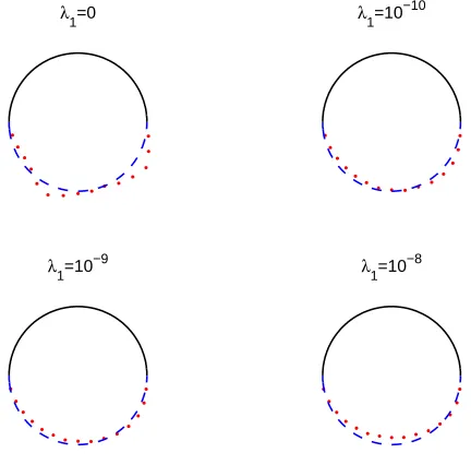
iterations are presented in Figures 12 and 13, respectively. From these figures, it can be seen that regularization with λ1 between 10−10

and 10−9

or with λ2 between10−1

and 100

produces stable and accurate reconstructions of the semicircular shape (4.2b).

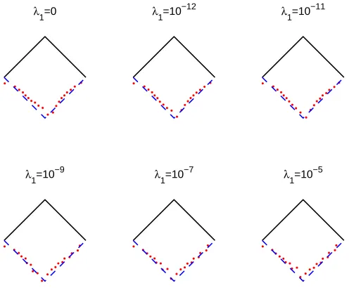
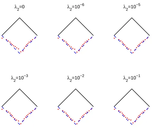
4.5. Example 5. We finally consider a square of side√2rotated byπ/4with boundaries∂Ω1and∂Ω2defined by ∂Ω1={x= (x, y)|0≤x≤1;y= 1−x} ∪ {x= (x, y)| −1≤x≤0;y= 1 +x}, (4.8a)

∂Ω2={x= (x, y)| −1≤x≤0;y=−1−x} ∪ {x= (x, y)|0≤x≤1;y=−1 +x}. (4.8b)

We considered the Neumann case α= 0, β= 1 and took the exact solution (4.1) with a= 1, b= i√a2_+κ2 _and κ= √2. The initial guess was(a0_,r0_{) = (0,0.65) and M = 21, N = 21, L= 20. The effects of regularization}

withλ1 orλ2, after 2000 iterations, forp= 10%noise are presented in Figures 14 and 15, respectively. From these figures, it can be seen that stable and accurate reconstructions of the right-angle wedge shape (4.8b) are obtained.

5. Conclusions

In this work, the PWM was successfully applied, apparently for the first time, for obtaining stable and accurate so-lutions of an inverse problem associated with two-dimensional Helmholtz-type equations, namely the reconstruction of an unknown portion of the boundary from a given exact boundary condition on this part of the boundary and additional noisy Cauchy data on the remaining known portion of the boundary. This inverse geometric problem is ill-posed and in discrete form yields an ill-conditioned system of nonlinear equations, which was solved, in a stable manner, by employing the Tikhonov regularization method [43]. The value of the regularization parameter was chosen according to Hansen’s L-curve criterion [18]. Five examples for two-dimensional simply connected, convex and non-convex domains and having smooth and piecewise smooth boundaries, were considered. From the numerical experiments, it can be concluded that the proposed method is stable with respect to noise in the Cauchy data. Furthermore, it is accurate and computationally very efficient. The application of the PWM for the detection of internal defects as well as to three-dimensional inverse geometric problems will be the subject of future research.

References

[1] C. J. S. Alves and S. S. Valtchev, Numerical simulation of acoustic wave scattering using a meshfree plane waves method, International Workshop on Meshfree Methods, 2003,http://www.math.ist.utl.pt/meshfree/silen.pdf.

[2] C. J. S. Alves and S. S. Valtchev,Numerical comparison of two meshfree methods for acoustic wave scattering, Eng. Anal. Bound. Elem.29_{(2005), 371–382.}

[3] P. R. S. Antunes,Numerical calculation of eigensolutions of 3D shapes using the method of fundamental solutions, Numer. Methods Partial Differential Equations27_{(2011), 1525–1550.}

[4] F. Berntsson, V. A. Kozlov, L. Mpinganzima and B. O. Turesson,An alternating iterative procedure for the Cauchy problem for the Helmholtz equation, Inverse Problems Sci. Eng.22_{(2014), 45–62.}

[5] F. Berntsson, V. A. Kozlov, L. Mpinganzima and B. O. Turesson,An accelerating alternating iterative procedure for the Cauchy problem for the Helmholtz equation, Comput. Math. Appl.68_{(2014), 44–60.}

[6] D. E. Beskos,Boundary element method in dynamic analysis: Part II (1986–1996), ASME Appl. Mech. Rev.50_{(1997), 149–197.}

[7] B. Bin-Mohsin and D. Lesnic,Identification of a corroded boundary and its Robin coefficient, East Asian J. Appl. Math.2_(2012),

126–149.

[8] D. Borman, D. B. Ingham, B. T. Johansson and D. Lesnic,The method of fundamental solutions for detection of cavities in EIT, J. Integral Equations Appl.21_{(2009), 381–404.}

[9] A. Borsic, B. M. Graham, A. Adler and W.R.B. Lionheart,Invivoimpedance imaging with total variation regularization, IEEE Trans. Med. Inaging29_{(2010), 44–54.}

[10] O. Cessenat and B. Després, Using plane waves as base functions for solving time harmonic equations with the ultra weak variational formulation, J. Comput. Acoustics11_{(2003), 227–238.}

[11] C. S. Chen, A. Karageorghis and Y. Li,On choosing the location of the sources in the MFS, Numer. Algor.72_{(2016), 107–130.}

[12] J. T. Chen and F. C. Wong,Dual formulation of multiple reciprocity method for the acoustic mode of a cavity with a thin partition, J. Sound Vibration217_{(1998), 75–95.}

[14] W. Chen, Z. J. Fu and X. Wei,Potential problems by singular boundary method satisfying moment condition, CMES – Comput. Model. Eng. Sci.54_{(2009), 65–85.}

[15] P. Debye and E. Hückel,The theory of electrolytes. I. Lowering of freezing point and related phenomena, Phys. Z.24_(1923),

185–206.

[16] G. Fairweather and A. Karageorghis,The method of fundamental solutions for elliptic boundary value problems, Adv. Comput. Math.9_{(1998), 69–95.}

[17] W. S. Hall and X. Q. Mao,A boundary element investigation of irregular frequencies in electromagnetic scattering, Eng. Anal. Bound. Elem.16_{(1995), 245–252.}

[18] P. C. Hansen,Rank-Defficient and Discrete Ill-Posed Problems: Numerical Aspects of Numerical Inversion, SIAM, Philadelphia, 1998.

[19] I. Harari, P. E. Barbone, M. Slavutin and R. Shalom,Boundary infinite elements for the Helmholtz equation in exterior domains, Int. J. Numer. Meth. Eng.41_{(1998), 1105–1131.}

[20] I. Herrera,Boundary Methods: An Algebraic Theory, Applicable Mathematics Series, Pitman (Advanced Publishing Program), Boston, MA, 1984.

[21] V. Isakov,Inverse obstacle problems, Inverse Problems25_{(2009), 123002 (18 pp).}

[22] B. Jin and L. Marin,The plane wave method for inverse problems associated with Helmholtz-type equations, Eng. Anal. Bound. Elem.32_{(2008), 223–240.}

[23] B. Jin and Z. Zheng,Boundary knot method for some inverse problems associated with the Helmholtz equation, Int. J. Numer. Meth. Eng.62_{(2005), 1636–1651.}

[24] D. S. Jones,Methods in Electromagnetic Wave Propagation, Oxford University Press, New York, 1979.

[25] S. I. Kabanikhin and M. A. Shishlenin,Stability analysis of a continuation problem for the Helmholtz equation, Bull. Novosibirsk Comp. Center16_{(2013), 59–63.}

[26] S. I. Kabanikhin, Y. S. Gasimov, D. B. Nurseitsov, M. A. Shishlenin, B. B. Sholpanbaev and S. Kasenov,Regularization of the continuation problem for elliptic equations, J. Inverse Ill-Posed Problems21_{(2013), 871–884.}

[27] B. Kaltenbacher, A. Neubauer and O. Scherzer, Iterative Regularization Methods for Nonlinear Problems, de Gruyter, Berlin, 2008.

[28] E. J. Kansa,Multiquadrics: A scattered data approximation scheme with applications to computational fluid dynamics, Comput. Math Appl.19_{(1990), 147–161.}

[29] A. Karageorghis,The plane waves method for axisymmetric Helmholtz problems, Eng. Anal. Bound. Elem.69_{(2016), 46–56.}

[30] A. Karageorghis and D. Lesnic,The method of fundamental solutions for the inverse conductivity problem, Inverse Problems Sci. Eng.18_{(2010), 567–583.}

[31] A. Karageorghis, D. Lesnic and L. Marin,A survey of applications of the MFS to inverse problems, Inverse Problems Sci. Eng.

19_{(2011), 309–336.}

[32] A. Karageorghis, D. Lesnic, and L. Marin, The MFS for inverse geometric problems, Inverse Problems and Computational Mechanics (L. Munteanu L. Marin and V. Chiroiu, eds.), vol. 1, Editura Academiei, Bucharest, 2011, pp. 191–216.

[33] A. D. Kraus, A. Aziz and J. Welty,Extended Surface Heat Transfer, John Wiley & Sons, New York, 2001. [34] P. D. Lax and R. S. Phillips,Scattering Theory, Academic Press, New York, 1967.

[35] J. Lian and S. Subramanian, Computation of molecular electrostatics with boundary element methods, Biophys. J.73_(1997),

1830–1841.

[36] X. Li,On solving boundary value problems of modified Helmholtz equations by plane wave functions, J. Comput. Appl. Math.195

(2006), 66–82.

[37] L. Marin,Numerical boundary identification for Helmholtz-type equations, Comput. Mech.39_{(2006), 25–40.}

[38] L. Marin and A. Karageorghis,Regularized MFS-based boundary identification in two-dimensional Helmholtz-type equations, CMC Comput. Mater. Continua10_{(2009), 259–293.}

[39] L. Marin, L. Elliott, P. J. Heggs, D. B. Ingham, D. Lesnic and X. Wen, Conjugate gradient-boundary element solution to the Cauchy problem for Helmholtz-type equations, Comput. Mech.31_{(2003), 367–377.}

[40] L. Marin, L. Elliott, P. J. Heggs, D. B. Ingham, D. Lesnic and X. Wen,BEM solution for the Cauchy problem associated with Helmholtz-type equations by the Landweber method, Eng. Anal. Bound. Elem.28_{(2004), 1025–1034.}

[41] The MathWorks, Inc., 3 Apple Hill Dr., Natick, MA,Matlab.

[42] Numerical Algorithms Group Library Mark 21 (2007), NAG (UK) Ltd, Wilkinson House, Jordan Hill Road, Oxford, UK. [43] A. N. Tikhonov and V. Y. Arsenin,Methods for Solving Ill-Posed Problems, Nauka, Moscow, 1986.

iter=10 iter=100

iter=1000 iter=2000

Figure 1. _{Example 1: Results for α= 1, β = 0 and no noise. The reconstructed boundary is} shown in red dots (· · ·).

iter=10 iter=100

iter=1000 iter=2000

iter=10 iter=100

iter=1000 iter=2000

Figure 3. _{Example 2: Results forα= 1, β= 0and no noise.}

iter=10 iter=100

iter=1000 iter=2000

iter=10 iter=100

iter=1000 iter=2000

Figure 5. _{Example 2: Results forα= 0, β = 1, noisep= 10%and no regularization.}

λ₁=0 λ₁=10−12 λ₁=10−10

λ₁=10−9 λ₁=10−7 λ₁=10−4

λ₂=0 λ

2=10

−6 _λ

2=10 −2

λ₂=10−1 λ₂=100 λ₂=101

Figure 7. _{Example 2: Results forα= 0, β= 1, noisep= 10%,λ1= 0and regularization withλ2.}

λ₁=0 λ₁=10−6 λ₁=10−5

λ₁=10−4 λ₁=10−3 λ₁=10−2

λ₂=0 λ

2=10

−3 _λ

2=10 −2

λ₂=10−1 λ₂=100 λ₂=101

Figure 9. _{Example 3: Results for noise p= 5%,λ1= 0and regularization withλ2.}

0.01 0.05 0.1

100 102

λ₁=10−3 λ₁=10−4

λ₁=10−2

||Residual||

2

||

a

|| 2

(a)

0.01 0.025 0.05

10−4 10−2 100

λ₂=50 λ₂=10

λ₂=10−1

||Residual||

2

||

r

′ || 2

(b)

iter=10 iter=100

iter=1000 iter=2000

Figure 11. _{Example 4: Results for no noise.}

λ₁=0 λ₁=10−10

λ₁=10−9 λ₁=10−8

λ₂=0 λ

2=10 −2

λ₂=10−1 λ

2=10 0

λ₁=0 λ

1=10

−12 _λ

1=10 −11

λ₁=10−9 λ₁=10−7 λ₁=10−5

Figure 14. _{Example 5: Results for noisep= 10%,λ2= 0 and regularization withλ1.}

Department of Mathematics and Statistics, University of Cyprus/Panepisthmio Kuprou, P.O. Box 20537, Nicosia/Leukwsia, Cyprus/Kuproc

E-mail address:[email protected]

Department of Applied Mathematics, University of Leeds, Leeds LS2 9JT, UK

E-mail address:[email protected]

Department of Mathematics, Faculty of Mathematics and Computer Science, University of Bucharest, 14 Academiei, 010014 Bucharest, and Institute of Mathematical Statistics and Applied Mathematics, Romanian Academy, 13 Calea 13 Septembrie, 050711 Bucharest, Romania

λ₂=0 λ

2=10

−6 _λ

2=10 −5

λ₂=10−3 λ₂=10−2 λ₂=10−1