Bayesian calibration and number of jump components in electricity spot price models

Version: Accepted Version Article:

Gonzalez, J, Moriarty, J and Palczewski, J orcid.org/0000-0003-0235-8746 (2017) Bayesian calibration and number of jump components in electricity spot price models. Energy Economics, 65. pp. 375-388. ISSN 0140-9883

https://doi.org/10.1016/j.eneco.2017.04.022

© 2017 Elsevier B.V. This manuscript version is made available under the CC-BY-NC-ND 4.0 license http://creativecommons.org/licenses/by-nc-nd/4.0/

eprints@whiterose.ac.uk Reuse

Items deposited in White Rose Research Online are protected by copyright, with all rights reserved unless indicated otherwise. They may be downloaded and/or printed for private study, or other acts as permitted by national copyright laws. The publisher or other rights holders may allow further reproduction and re-use of the full text version. This is indicated by the licence information on the White Rose Research Online record for the item.

Takedown

If you consider content in White Rose Research Online to be in breach of UK law, please notify us by

PII: S0140-9883(17)30129-9

DOI: doi:10.1016/j.eneco.2017.04.022

Reference: ENEECO 3622 To appear in: Energy Economics

Received date: 10 February 2016 Revised date: 20 April 2017 Accepted date: 28 April 2017

Please cite this article as: Gonzalez, Jhonny, Moriarty, John, Palczewski, Jan, Bayesian calibration and number of jump components in electricity spot price models, Energy Economics(2017), doi: 10.1016/j.eneco.2017.04.022

ACCEPTED MANUSCRIPT

Bayesian calibration and number of jump components in

electricity spot price models

Jhonny Gonzaleza_{, John Moriarty}b_{, Jan Palczewski}1c

a_{School of Mathematics, University of Manchester, Manchester M13 9PL, UK} b_{School of Mathematical Sciences, Queen Mary University of London, London E1 4NS, UK}

c_{School of Mathematics, University of Leeds, Leeds LS2 9JT, UK}

Abstract

We find empirical evidence that mean-reverting jump processes are not statistically adequate to model electricity spot price spikes but independent, signed sums of such processes are sta-tistically adequate. Further we demonstrate a change in the composition of these sums after a major economic event. This is achieved by developing a Markov Chain Monte Carlo (MCMC) procedure for Bayesian model calibration and a Bayesian assessment of model adequacy (poste-rior predictive checking). In particular we determine the number of signed mean-reverting jump components required in the APXUK and EEX markets, in time periods both before and after the recent global financial crises. Statistically, consistent structural changes occur across both markets, with a reduction of the intensity and size, or the disappearance, of positive price spikes in the later period. All code and data are provided to enable replication of results.

Keywords: Multi-factor models, Bayesian calibration, Markov Chain Monte Carlo, Ornstein-Uhlenbeck process, Electricity spot price, Negative jumps

1. Introduction

Electricity spot markets have multiple fundamental drivers, for example baseload and renew-able production (Würzburg et al., 2013). Disturbances in these drivers, such as plant outages and renewable gluts, can clearly have different dynamic characteristics and consequences. Since sharp disturbances create spikes in electricity spot prices (Seifert and Uhrig-Homburg, 2007) we may hypothesise that, over time, disturbances in different drivers give rise to spikes with sta-tistically distinguishable directions, frequencies, height distributions and rates of decay. It has recently been demonstrated that electricity spot price formation can evolve over time (Brunner, 2014). Thus we may also hypothesise that the statistical characteristics of electricity price spikes

ACCEPTED MANUSCRIPT

will evolve in step with underlying economic events and developments, such as shifts in demand and increasing renewable penetrations.

In this paper we find empirical support for these two hypotheses. To this end we use multi-factorelectricity spot price models, with multiple superposed mean-reverting components and a seasonal trend (Benth et al., 2007). This allows statistical patterns such as mean reversion, sea-sonality and spikes to be reproduced in modelling. Crucially for the present study, this approach also allows the statistical modelling of multiple spike components with differing frequencies, height distributions, decay rates, and directions (positive or negative). We demonstrate that in some electricity markets two types of positive spike are observed, while other markets require the inclusion of negative spikes. The modelling of negative spikes is an area of emerging in-terest (Fanone et al., 2013) as renewable penetrations, and hence gluts in renewable production, increase. Finally we document evolution of the statistical spike structure through periods of eco-nomic change by comparing two markets across two time periods, one before the recent global financial crises (2000-2007) and another afterwards (2011-2015) and reflect on possible inter-pretations of the results.

The calibration of multi-factor models is a highly challenging task and existing approaches typically involve making stronga prioriassumptions, such as setting thresholds for jump sizes, which may mask the true statistical structure. Methodologically, we develop a Bayesian ap-proach to calibration based on Markov Chain Monte Carlo (MCMC) methods. This goes beyond previous work by making minimal assumptions and enables us, for example, to estimate mod-els with multiple spike components acting in the same direction, a feature which is confirmed empirically (in 2001–2006 data from the APXUK electricity spot market). In order to assess the number of mean-reverting jump components required we perform a Bayesian procedure of

posterior predictive checking.

1.1. Background and related work

ACCEPTED MANUSCRIPT

The complexity of electricity spot price models, and multi-factor models in particular, makes their analysis statistically challenging and has given rise to a substantial literature. A single-factor model including the above stylised features was introduced by Clewlow and Strickland (2000). Through the use of a threshold, the single-factor model of Geman and Roncoroni (2006) incorporates two jump regimes: when the price is below the threshold jumps are positive, and when the price exceeds the threshold jumps are negative. Beginning with Lucia and Schwartz (2002) multi-factor models have expressed the price as a sum of unobservable or latent pro-cesses (factors) with distinct purposes, for example the modelling of short-term and long-term price variations respectively. Unlike many single factor models, multifactor models do not im-ply a perfect correlation between changes in spot, future and forward prices, which is consistent with the non-storability of electricity (Benth and Meyer-Brandis, 2009). The model of Lucia and Schwartz (2002) has two factors, namely a Gaussian mean-reverting process and an arithmetic Brownian motion (that is, a scaled Brownian motion with drift). Interestingly, while also de-veloping a two-factor model, Seifert and Uhrig-Homburg (2007) explicitly refer to the physical origins of various types of jumps. Beyond two-factor models, a simple and flexible multi-factor model with jumps is given in Benth et al. (2007). Estimation procedures for this model are dis-cussed in Meyer-Brandis and Tankov (2008), although the latter work adds strong assumptions in order to obtain tractable methods.

The interdependency between parameters in multi-factor models, in particular, is a challenge to calibration methods. A straightforward approach is to first separate the observed values into factors using signal filtering techniques, in order to subsequently employ classical maximum likelihood estimation. Such methods effectively assume that some of these interdependencies may be neglected, and this approach is taken for example in Meyer-Brandis and Tankov (2008) and Benth et al. (2012). An alternative is the joint estimation of latent factors, for which there are two leading methodologies in the literature: expectation-maximisation (EM)andMarkov Chain Monte Carlo (MCMC)methods. While EM produces point estimates for parameters in either a Bayesian or frequentist framework2 _{(see, for example, Rydén et al. (2008)), MCMC is able to}

generate samples from posterior parameter distributions. Particularly in models with multiple parameters and latent processes, these interdependencies may result in likelihood surfaces and

2_{Two possible approaches to the calibration of model parameters are commonly referred to asfrequentistand}

ACCEPTED MANUSCRIPT

posterior distributions which are rather flat around their maxima. While EM suffers from Monte Carlo errors which amplify the usual difficulties in numerical optimisation for such problems, MCMC estimates the posterior distribution providing an analyst with a more complete picture of the interrelations between parameters.

In related contexts, MCMC has been applied to fit continuous-time stochastic volatility mod-els to financial time series, where the price is a diffusion process whose volatility is a latent mean reverting jump process or the sum of a number of such processes (called a superposition model). In this line of research a missing data methodology is employed whereby the observed pro-cess is augmented with one or more latent marked Poisson propro-cesses and the MCMC procedure generates posterior samples in this high dimensional augmented state space. Examples include Roberts et al. (2004), Griffin and Steel (2006) and Frühwirth-Schnatter and Sögner (2009). Since energy prices additionally exhibit jumps directly in their paths, MCMC has been applied to ex-tensions of these models in which a diffusion process with stochastic volatility is superposed with a jump process, see Green and Nossman (2008) in the context of electricity and Brix (2015) for gas prices. Technically the latter two papers estimate a discrete approximation of the models whereas in this study we pursueexactinference for continuous time models.

1.2. Contribution

From the modelling point of view a novelty of the present study is that the price is a super-position of more than one jump component, each with its own sign, frequency, size distribution and decay rate, along with a diffusion component. This approach acknowledges that the negative price spikes attributable to rapid wind power fluctuations may, for example, have quicker decay than the infrequent larger positive spikes due to major disturbances such as outages of a tradi-tional generation plant. The inclusion of multiple jump components also addresses the following problem identified in Green and Nossman (2008) and Brix (2015). In two-factor models jumps of intermediate size must be accounted for either in the diffusion process (forcing unlikely spikes in the Brownian motion path) or the jump process (implying additional jumps). While the for-mer can lead to an overestimation of volatility in the diffusion process, the latter may result in an overestimation of the intensity of the jump process, which is independent of the jump sizes. The inclusion of a second jump process with its own mean jump size and rate of mean reversion removes this dichotomy, offering an alternative to the inclusion of stochastic volatility in the diffusion process.

ACCEPTED MANUSCRIPT

approximation to continuous dynamics. While this approximation is often used for practical rea-sons including simplified and/or tractable implementation, it is not possible to assess a priori the extent of the estimation error introduced by the approximation employed. Our MCMC pro-cedure is not based on time discretisation of the model and the inference is therefore exact at the level of distributions. This is in contrast with the work in the aforementioned papers (Seifert and Uhrig-Homburg, 2007; Green and Nossman, 2008; Brix, 2015). Despite the relative sim-plicity of our multi-factor model, the MCMC procedure involves a number of challenging issues and in the electronic appendix we provide additional comments and details concerning efficient implementation.

In addition we demonstrate that model adequacy may also be addressed by our MCMC method. The complexity of electricity spot price models naturally gives rise to parsimony con-siderations. While multi-factor models (potentially also including latent volatility processes) offer great flexibility, the potential statistical pitfalls of overly flexible models, for example re-lating to issues of identifiability and out-of-sample prediction, are well known. In this context, the ability of MCMC to sample whole trajectories from the posterior distribution of the jump processes means in particular that the adequacy of latent variable models may be addressed. We exploit this fact by using the MCMC procedure to perform posterior predictive checks in the sense of Rubin (1984). For two different electricity spot markets, over two different periods of time, we determine in this way the minimum number of superposed processes required in the model. We find that two or three factors are sufficient in each case. We also show that taking either constant or periodic deterministic jump intensity rates can provide a relatively simple but sufficiently flexible modelling palette. Since the jump processes influence the spot price directly (additively) and have their own proper dynamics such models are also rather interpretable. More generally, since multi-factor models have been considered for a range of commodities including oil and gas (Schwartz and Smith, 2000; Brix, 2015) our algorithm is also potentially applicable in these contexts although this is outside the scope of the present paper (see Gonzalez (2015, Chapter 5) for an application to gas prices).

Section 2 describes the model and the data which animates our study, while Section 3 presents our MCMC algorithm including the approach to assessing model adequacy through posterior predictive checking. The data is analysed in Section 4. Section 5 contains discussion of results and Section 6 concludes. Notes on the efficient implementation of the algorithm are provided in the electronic appendix. Throughout we denote probability distributions as follows: N(a, b)

denotes the Normal distribution with mean a and variance b, Ga(a, b) the Gamma distribution

ACCEPTED MANUSCRIPT

Jan 2001 Jan 2002 Jan 2003 Jan 2004 Jan 2005 Jan 2006 Jan 2007Jan 2011 Jan 2012 Jan 2013 Jan 2014 Jan 2015 0

1 2 3 4 5 6

£/MWh

Deseasonalised APXUK

Jan 2001 Jan 2002 Jan 2003 Jan 2004 Jan 2005 Jan 2006 Jan 2007Jan 2011 Jan 2012 Jan 2013 Jan 2014 Jan 2015 -2

0 2 4 6 8 10

Deseasonalised EEX

Figure 1: Deseasonalised APXUK (top panel) and EEX (bottom panel) daily average prices (excluding weekends) over two periods. The first period starts on March 27, 2001 for APXUK and on June 16, 2000 for EEX and finishes on November 21, 2006 for both markets. The second period is January 24, 2011 to February 16, 2015 for both series. Details of the deseasonalisation procedure are given in the electronic appendix.

the Exponential distribution with mean a and U(a, b) the Uniform distribution on the interval (a, b).

2. Model

2.1. Motivation

ACCEPTED MANUSCRIPT

demand, although the picture across Europe was mixed.3 _{In order to reveal the structure of these}

price series more clearly the four time series have been separately deseasonalised (for details see the electronic appendix).

Reversion to a constant level is strongly suggested in the EEX data (bottom panel) and also, to a slightly lesser extent, in the APXUK series (top panel). Taking first the 2001–2006 APXUK data, the presence of significant positive price spikes is clear. However visual inspection also suggests that while some spikes decayed very quickly, a significant number showed more gradual decay. In contrast the positive spikes in the 2000–2006 EEX data appear uniformly to decay quickly and, in addition, the presence of smaller but rather frequent negative spikes is suggested. While the 2011–2015 APXUK data also suggests regular positive spikes, their heights are significantly smaller than those observed in 2001–2006. In the 2011–2015 EEX data the presence of negative spikes is suggested perhaps more strongly than in 2000–2006. Further, once these negative spikes are taken into account, visual inspection reveals apparently little evidence of positive spikes.

For each series we apply the MCMC procedure described in Section 3 to verify the conclu-sions of our visual analysis and to establish the smallest number of signed jump components for which the posterior predictive check is favourable, in a sense made precise in Section 4.

In the following subsections we present in detail the class of spot price models to be cali-brated.

2.2. Ornstein-Uhlenbeck processes

A processY(t), 0 _≤ t _≤ T which is right continuous with left limits is called an

Ornstein-Uhlenbeck (OU) process if it is the unique strong solution to the stochastic differential equation (SDE)

dY(t) = λ−1(µ₋Y(t))dt+σdL(t), Y(0₋) = y0, (1)

where L(t) is a driving noise process with independent increments, ie., a Lévy process. The

initial state of the process Y is defined as the value at the left-hand limit Y(0₋) due to the

possibility of a jump at time 0. In equation (1),µ _{∈ R}is the mean level to which the process

tends to revert,λ−1 _{> 0}denotes the speed of mean reversion and_{σ > 0}is the volatility of the

3_{Sources: European Commission Eurostat service; Digest of United Kingdom Energy Statistics (DUKES) 2015,}

ACCEPTED MANUSCRIPT

OU process. The unique strong solution to the SDE (1) is given by

Y(t) =µ+ (y0−µ)e−λ

−1

t₊  t

0

σe−λ−1

(t−s)_dL(s). (2)

We consider two different specifications for the Lévy processL(t)drivingY(t). On the one

hand we consider an OU process whereL(t) = W(t)is a standard Wiener process. In this case

the conditional distribution ofY(t+s)givenY(t),t _∈[0, T],s_∈[0, T ₋t], is Normal with the

mean

E[Y(t+s)_|Y(t) =y] = µ+ (y₋µ)e−λ−1s,

and the variance

V ar[Y(t+s)_|Y(t) =y] = λσ2(1₋e−2λ−1s)/2.

Hence we call the processY(t)a Gaussian OU process. On the other hand we consider the case

whereL(t)is a compound Poisson process, with theinterval representation

L(t) =

∞

j=1

ξj1{t≥τj}, (3)

where the τj are the arrival times of a Poisson process and ξj represents the jump size at time τj (these jump sizes are independent and identically distributed (i.i.d.) random variables). The

dynamics ofY(t)are explicitly given by

Y(t+s) =µ+ (Y(t₋)₋µ)e−λ−1s+

j:t≤τj≤t+s

e−λ−1(t+s−τj)_{ξj, s}

≥0. (4)

Below we shall model the stochastic part of energy spot prices by superimposing a number of OU processes.

2.3. A multi-factor model for energy spot prices

Let us denote byX(t)the de-trended and deseasonalised spot price at timet _≥0

(presenta-tion of the rela(presenta-tion betweenX(t)and the electricity spot priceS(t)is deferred until the end of

this section). We assume that the deseasonalised priceX(t)is a sum ofn+ 1OU processes

X(t) = n

i=0

ACCEPTED MANUSCRIPT

whereY0 is a Gaussian OU process

dY0(t) = λ−₀1(µ₋Y0(t))dt+σdW(t), Y0(0) =y0, (6)

and eachYi, i_≥1is a jump OU process

dYi(t) = ₋λ−_i 1Yi(t)dt+dLi(t), Yi(0₋) = yi, i= 1, . . . , n, (7)

each Li being a (possibly inhomogeneous) compound Poisson process with exponentially

dis-tributed jump sizes having meanβi. We will refer to this as the(n+1)-OUmodel. The constants wi _{∈ {}1,₋1_}are used to indicate whether positive or negative jumps are being modelled. Notice

that each of the processes Yi(t), i _≥ 1, is non-negative since the Li are increasing processes.

Thus by setting wi = 1, we employ Yi(t) to capture positive price spikes, whereas by setting wi = ₋1, Yi(t) is assumed to model negative price spikes. Throughout we assume that w0 is

equal to 1.

For each compound Poisson processLi, i _≥ 1, we consider one of two specifications of the

jump intensity rate. In the simpler specification we assume that the intensity rate is constant and equal toηi, and hence that jump frequency is independent of time. In the alternative specification

we take account of periodicity in the jump rate as in Geman and Roncoroni (2006) through the deterministic periodic intensity function

Ii(ηi, θi, δi, t) =ηi !

2

1 +_|sin(π(t₋θi)/ki)_| −1

"δi

, (8)

which has periodkidays, whereki _∈(0,_∞)(see Figure 2 for a graph of the fitted intensity

func-tionI1). The parameterηi ∈ (0,∞)is the maximum jump rate whilst the exponentδi ∈(0,∞)

controls the shape of the periodic function. In order to have a compact notation covering both the above model specifications, the intensity function parameter vector associated with the processYi

will simply be denotedϑi. In the constant intensity model specification we therefore understand

thatϑi =ηi, while in the periodic intensity model it is understood thatϑi = (ηi, θi, δi).

We aim to show that using the sum of a number of such OU processes provides suitable flexibility for modelling electricity spot prices. A diffusive Gaussian component is used to model regular trading characterised by frequent small price variations. The jump components model the arrival of temporary system disturbances of various kinds causing imbalance between supply and demand. By specifying two jump components, say, such that λ1 > λ2, we can capture slowly

ACCEPTED MANUSCRIPT

1 2 3 4 5 6

Average

Fitted intensity function 20

Figure 2: Monthly average number of positive jumps on the EEX market during 2000-6, together with the intensity functionI1with parameter values taken from Table 4 for the 3-OU-I1model. As the jumps are not directly

observ-able in the spot price series, we report the numbers inferred from the latent jump processes sampled in the MCMC procedure.

decay rates may correspond to differentphysical causes of spikes such as power plant outages or extreme changes in weather. The possibility of incorporating negative price spikes by taking

wi =₋1is explored in Section 4.

In the empirical studies of Section 4 we assume that the relation between the spot priceS(t)

and the deseasonalised priceX(t)is of the following form:

S(t) =ef(t/260)X(t), (9)

where f : [0,_∞) _→ Ris a deterministic function that captures the long-term price trend and seasonality typically observed in energy spot prices. In our analysis we take a day as the unit of time and skip weekends due to their distinctly different price dynamics, resulting in a 260-day year. The function f is specified in terms of years to capture weather-induced market patterns

linked to seasonal variations. The multiplicative seasonality in (9) is in line with the exponential price trends standard in mathematical economics. We take

f(τ;a1, . . . , a6) =a1+a2τ+a3sin(2πτ) +a4cos(2πτ) +a5sin(4πτ) +a6cos(4πτ), (10)

ACCEPTED MANUSCRIPT

3. Inference

In this section we present a Markov Chain Monte Carlo (MCMC) approach to Bayesian inference in the superposition model (5). We construct a Markov chain whose stationary distri-bution is the posterior distridistri-bution of the parameters in our model together with latent variables introduced to make the inference computationally tractable, see Section 3.1. The application of a Gibbs sampler allows single parameters or groups thereof to be updated conditioned on oth-ers being fixed – a standard MCMC approach which aids computational tractability. Central to the performance of MCMC and particularly the Gibbs sampler is the notion ofmixingwhich is linked to the speed of convergence of the chain to its stationary distribution. Intuitively the better the mixing, the smaller the dependence between consecutive steps of the chain and, in effect, the less the chain gets blocked in small areas of the state space for long stretches of time. Mixing is negatively affected when the parameters which are updated at a given step of a Gibbs sampler depend on those upon which they are conditioned. This will be of particular importance in the choice of latent variables.

In Sections 3.1-3.3 we present techniques for Bayesian inference in the superposition model (5) in the case of one jump OU component (n = 1). This is then extended in Section 3.4 to the

case of multiple jump components. For simplicity, when it does not lead to ambiguity, we drop the subscript in the jump processL1 and its parameters, so thatL=L1,β =β1andϑ=ϑ1. 3.1. Data augmentation

LetX =_{x0, . . . , xN_}denote observations of the process (5) at times0 = t0, . . . , tN =T,

and ∆i = ti − ti−1 > 0, i = 1, . . . , N, the time increments between consecutive

observa-tions. The likelihood ℓ(_{X |} µ, λ0, σ, λ1, ϑ, β) of the data given parameters is neither

analyti-cally tractable nor amenable to numerical integration since it involves an infinite sum of inte-grals over high dimensional spaces. However by augmenting the state space with observations

Y1 ={y1,0, . . . , y1,N}of the processY1 at timesti, the likelihood ofX givenY1 becomes

inde-pendent ofλ1, ϑ andβ. Thanks to the explicit form of the transition density of a Gaussian OU

process we have

ℓ(_{X |} µ, λ0, σ,_Y1) = N #

i=1 1 √

2πΣi exp

$ −_2Σ12

i %

zi₋µ₋(zi−1−µ)e−λ

−1 0 ∆i

&2'

, (11)

whereΣ2

i =λ0σ2(1−e−2λ

−1

0 ∆i)/2and

ACCEPTED MANUSCRIPT

Space augmentation methods have been widely used in statistics to tackle computationally infeasible problems. However the choice of latent variables or processes has a profound influence on the properties of the resulting estimators, affecting in particular the mixing of a Markov chain approximating the posterior distribution. From a mathematical point of view, the body of work closest to the present inference problem is estimation in the context of stochastic volatility models, where the volatility process is driven by a jump process. Among these are the state space augmentations used in (Jacquier et al., 1994; Kim et al., 1998) and later criticised by Barndorff-Nielsen and Shephard (2001, p. 188) for high posterior correlation of the parameterλ1 with the

input trajectory of the processY1. This correlation could lead to MCMC samplers based on this

parametrisation performing poorly. Instead, Barndorff-Nielsen and Shephard (2001) propose an alternative data augmentation scheme based on a series representation of integrals with respect to a Poisson process L(t), known as the Rosi´nski or Ferguson-Klass representation. Bayesian

inference for a stochastic volatility model under this parametrisation was first explored in the discussion section of Barndorff-Nielsen and Shephard (2001) and further developed in Griffin and Steel (2006) and Frühwirth-Schnatter and Sögner (2009). In the present paper, however, we opt for the following more direct parametrisation independently suggested by several researchers (see, for example, Barndorff-Nielsen and Shephard (2001) and Roberts et al. (2004)).

Recall from Section 2.3 that the process L(t) driving Y1(t)is a compound Poisson process

with intensity functionI(ϑ, t)and interval representation (3). Recall also that

Y1(t+s) =Y1(t₋)e−λ−11s+

j:t≤τj≤t+s

e−λ−11(t+s−τj)_{ξj, s≥0,} (13)

which motivates a data augmentation methodology where the set of pairs {(τj, ξj)}, instead of

the processY, is treated as the missing data. This has the benefit of introducing independence

betweenλ1 and the latent variables, thus improving the mixing in Gibbs samplers.

Let us denote byΦthe marked Poisson process onS = [0, T]_×(0,_∞)with locationsτi on [0, T] and marksξi on(0,_∞). The probability density ofΦis defined relative to a dominating measure, namely that of a Poisson process with unit intensity on[0, T]and exponential jump sizes

with parameter 1. Hence, thanks to the marking theorem (Kingman, 1992) and the likelihood

ratio formula in Kutoyants (1998), the density ofΦwith respect to this dominating measure is

ℓ(Φ _|ϑ, β) =L(ϑ; Φ)_·β−NT _exp

(

−(β−1₋1) NT

j=1

ξj), (14)

ACCEPTED MANUSCRIPT

process with unit intensity, of the Poisson process with intensityI(ϑ, t):

L(ϑ; Φ) = exp

*_NT 

j=1

logI(ϑ, τj)₋ T

0

I(ϑ, t)dt+T !

. (15)

WhenLis a homogeneous Poisson process with constant intensityηwe obtain

L(ϑ;Φ) = exp"

−(η₋1)T#

ηNT_. (16)

We will use a Gibbs sampler to simulate from the posterior distribution of the parameters and the missing dataΦgiven the observed data_X, using the factorisation

π(µ, λ0, σ, λ1, ϑ, β,Φ_{| X})∝ℓ(X | µ, λ0, σ, λ1,Φ)ℓ(Φ|ϑ, β)π(µ, λ0, σ, λ1, ϑ, β), (17)

whereπ(µ, λ0, σ, λ1, ϑ, β)is the joint prior density of the parameters.

3.2. Classes of prior distributions

To complete our Bayesian model we now specify classes of prior distributions for the param-eters, which are assumed to be mutually independent4_{. For computational efficiency the classes}

chosen correspond to conjugate priors where possible. In the empirical studies presented in Sec-tion 4 the prior distribuSec-tions are chosen with a large spread (for example variance, where this exists) in order tolet the data speak for itself. Prior expectations are based on existing results in the literature, combined with further exploratory analysis of historical data as necessary. For de-tails see the electronic appendix. Of course users of our methodology may also have prior beliefs about the model parameters, and in our Bayesian context the prior distributions may alternatively be chosen to reflect these beliefs where appropriate.

We specify a N(aµ, b2µ)prior distribution for the mean levelµof the Gaussian OU component,

an IG(aσ, bσ)for its volatilityσ2, an IG(aβ, bβ)for the jump size parameterβand an IG(aλi, bλi) for the mean reversion parameter λi, i = 0,1. For the intensity function a Ga(aη, bη) prior

is chosen for η. Further when the intensity is periodic, a Ga(aδ, bδ) prior is taken for δ and a

U(aθ, bθ)prior forθ (cf. (8)).

4_{In Section 3.4 and following, where more than one jump OU component is considered, the only statistical}

dependence we assume is a strict ordering of the mean reversion parametersλj,j = 1, . . . , nwhen this is needed

ACCEPTED MANUSCRIPT

In the algorithm below the Gibbs step for updating theλiemploys a random-walk

Metropolis-Hastings procedure. To ensure that the mixing is of the same order for small and large values of

λi the step of the proposal should be state dependent; equivalently an appropriate transformation

ofλi may be applied. For computational convenience we opt for the latter, swappingλi in the

inference procedure withρi =e−λ−1

i .

After setting the initial state of the chain, the MCMC algorithm applied below cycles through the following steps:

MCMC algorithm for the 2-OU model

Step 1: updateµ∼π(µ|ρ0, σ, ρ1,X,Φ) Step 2: updateσ2 _∼π(σ2 _{|ρ0, ρ1,X,Φ)}

Step 3: updateρ0, ρ1 ∼π(ρ0, ρ1 |µ, σ,X,Φ)

Step 4: updateϑ ∼π(ϑ|Φ) Step 5: updateβ ∼π(β |Φ)

Step 6: updateΦ∼π(Φ |µ, ρ0, σ, ρ1, ϑ, β,X) Step 7: Go to step 1.

Below we provide more details about each of these steps.

Step 1. Updateµ

Recalling (11), the likelihood of the observed data conditional on the augmented state(µ, λ0, σ, ρ1,Φ)is

ℓ(X |µ, λ0, σ, ρ1,Φ) ∝

1

$N i=1Σi

exp % −1 2 N  i=1 1 Σ2 i &

zi−zi−1e−λ

−1 0 ∆i _+µ

& e−λ−1

0 ∆i₋₁

''2 !

,

whereΣ2

i =λ0σ2(1−e−2λ

−1

0 ∆i)/2and thez

i are computed as the difference between the

obser-vations ofXand the trajectory ofY implied by the realisationΦof the marked Poisson process. Using the conjugate prior forµspecified in the previous section it can be easily shown that the

conditional distributionπ(µ|ρ0, σ, ρ1,X,Φ)is

N    +N i=1 &

1−e−λ−1 0 ∆i

'

Σ−_i2&zi−zi−1e−λ

−1 0 ∆i

'

+aµ

σ2 0

+N i=1

&

1−e−λ−1 0 ∆i

'2

Σ−_i 2+ 1

b2 µ , 1 +N i=1 &

1−e−λ−1 0 ∆i

'2

Σ−_i 2+ 1

b2

µ



ACCEPTED MANUSCRIPT

Step 2. Updateσ2

Due to the choice of prior, the conditional distribution π(σ2 _{| ρ0, ρ1,X,Φ)} has the closed

form

IG

/ N

2 +aσ, 1

λ0

N 

i=1

si

(1₋e−2λ−1 0 ∆i)

+bσ 0

,

where

si = &

zi−zi−1e−λ

−1 0 ∆i _+µ

& e−λ−1

0 ∆i₋₁

''2 .

Step 3. Updateρ0andρ1

Explicit conditional distributions forρ0andρ1are not available and the density is only known

up to a multiplicative constant:

π(ρ0 |µ, σ, ρ1,X,Φ)∝ℓ(X | µ, ρ0, σ, ρ1,Φ)π(ρ0),

π(ρ1 |µ, σ, ρ0,X,Φ)∝ℓ(X | µ, ρ0, σ, ρ1,Φ)π(ρ1).

Hence we use a random-walk Metropolis-Hastings within Gibbs procedure to updateρ0 andρ1.

The variance of the proposal distribution is tuned after pilot runs in order to achieve an acceptance rate between20%and50%.

Step 4. Updateϑ

In the case of constant intensity function, the conjugate prior forη yields an explicit

condi-tional distribution

η |Φ∼Ga(aη +NT, T +bη).

When the intensity function is time dependent we employ a random-walk Metropolis-Hastings within Gibbs procedure to updateη, θandδ:

π(η, θ, δ |Φ) ∝ℓ(Φ |η, θ, δ)π(η)π(θ)π(δ).

ACCEPTED MANUSCRIPT

Step 5. Updateβ

The conditional distribution ofβ givenΦhas the closed form

β _|Φ∼IG

/

aβ+NT, NT



i=1

ξi+bβ 0

.

Step 6. Update the latent processΦ

The Metropolis-Hastings step we use to update the processΦdraws from the work of Geyer and Møller (1994), Roberts et al. (2004) and Frühwirth-Schnatter and Sögner (2009) on MCMC techniques for simulating point processes, extending it where appropriate to the case of inhomo-geneous Poisson processes.

Let us assume that the current state of the Markov chain is

Φ ={(τ1, ξ1), . . . ,(τNT, ξNT)},

that is, there areNT points on the setS with jump times given byτj and the corresponding jump

sizes byξj. We choose randomly, with equal probability, one of the following three proposals.

Birth-and-death step

In the birth-and-death step we choose one of two moves. With probabilityp∈(0,1)we choose a birth move whereby a new-born point (τ, ξ) is added to the current configuration of Poisson points. The proposed new state is thenΦ∪ {(τ, ξ)}. The pointτ is drawn uniformly from[0, T], whilstξ is drawn from the jump size distribution Ex(β). For this move the proposal transition kernel q(Φ,Φ ∪ {(τ, ξ)}) has the following density with respect to the product of Lebesgue measure on[0, T]and Ex(1)measure on(0,∞):

q(Φ,Φ∪ {(τ, ξ)}) =β−1exp1

−(β−1−1)ξ2 .

With probability1−pa death move is selected, a randomly chosen point(τi, ξi)being removed fromΦ(provided thatΦis not empty). The proposal transition kernel (with respect to the count-ing measure) is

q(Φ,Φ\ {(τi, ξi)}) = 1

NT,

where NT is the number of points in Φ before the death move. Then the Metropolis-Hastings acceptance ratio for a birth move fromΦtoΦ∪ {(τ, ξ)}is

ACCEPTED MANUSCRIPT

while the acceptance ratio for a death move fromΦtoΦ_{\ {}(τi, ξi)_}is

α(Φ,Φ_{\ {}(τi, ξi)}) = min %

1, 1

r1

Φ_{\ {}(τi, ξi)_},(τi, ξi)2 !

,

where

r( ˜Φ,(τ, ξ)) = ℓ(X | µ, ρ0, σ, ρ1,Φ˜∪ {(τ, ξ)})

ℓ(X |µ, ρ0, σ, ρ1,Φ)˜

π( ˜Φ∪ {(τ, ξ)} |ϑ, β)

π( ˜Φ|ϑ, β)

1−p p

× 1

(NT + 1)q(Φ,Φ∪ {(τ, ξ)})

= ℓ(X | µ, ρ0, σ, ρ1,Φ˜∪ {(τ, ξ)})

ℓ(X |µ, ρ0, σ, ρ1,Φ)˜

1−p p

T

˜

NT + 1I(ϑ, τ),

where_NT˜ is the number of points of_Φ˜, cf. (14).

Local displacement move

Without loss of generality let us assume that the jump times of the Poisson process are ordered, so thatτ1 <· · ·< τNT. In the local displacement move we choose randomly one of the jump times, sayτj, and generate a new jump timeτ uniformly on[τj−1, τj+1], puttingτ0 = 0andτNT+1 =T. The point (τj, ξj) is then displaced and re-sized to (τ, ξ), whereξ = e−λ

−1 1 (τ−τj)ξ

j. Formally

we choose uniformly one ofNT transition kernels, with thej-th one preserving the conditional

distribution π(τ, ξ|X, µ, ρ0, σ, ρ1, ϑ, β,Φ\{(τj, ξj)}). The proposal for the j-th kernel has the

Uniform distribution over(τj−1, τj+1)for the first variable with the second variable being then a

deterministic transformation given by a 1-1 mappingT(ξ, τ, τ′_{) = (ξe}−λ−1

1 (τ′−τ), τ′, τ)such that

T =T−1. Following Tierney (1998, Section 2), the contribution of this deterministic transition

to the Metropolis-Hastings acceptance ratio is|det∇T(ξj, τj, τ)|, whereτ is the new proposed

location of the jump. Hence the complete Metropolis-Hastings acceptance ratio is

r(Φ,Φnew) =

ℓ(X |µ, ρ0, σ, ρ1,Φnew) ℓ(X |µ, ρ0, σ, ρ1,Φ)

π(τ, ξ|ϑ, β)

π(τj, ξj|ϑ, β) ˜

q(τ, τj) ˜

q(τj, τ)|det∇T(ξj, τj, τ)|

= ℓ(X |µ, ρ0, σ, ρ1,Φnew)

ℓ(X |µ, ρ0, σ, ρ1,Φ)

I(ϑ, τ)

I(ϑ, τj)

e−β−1

ξ

e−β−1_ξ

je

−λ−11(τ−τj)_,

whereq˜(τ, τ′_{) = (τj+1 −τj−1)}−1 is the transition density for the jump location with respect to

ACCEPTED MANUSCRIPT

In this step the sizes of all jumps are independently updated. Specifically, for each jump(τj, ξj)

we propose a new jump sizeξ′

j =ξjφj, wherelog(φj)∼N(0, c2)are i.i.d. random variables. The

variancec2is chosen inversely proportional to the current number of jumps, and the performance

of this update step appears rather insensitive to the constant of proportionality. Denoting byΦnew

the Poisson point process with updated jump sizes, the Metropolis-Hastings acceptance ratio for this move is

α(Φ,Φnew) = min %

1,ℓ(X |µ, ρ0, σ, ρ1, ϑ, β,Φnew) ℓ(X | µ, ρ0, σ, ρ1, ϑ, β,Φ) exp

%

−(β−1−1)

NT



i=1

(ξ′ i−ξi)

! _N

T

3

i=1 ξ′

i ξi

! .

Note that the product$NT

i=1 ξ′i

ξi is equivalent to

$NT

i=1φi.

3.4. Bayesian inference for a sum of three OU processes

As discussed in Section 2.3 we may believe a priori that the price spikes observed in the market are of a certain number of types, corresponding to their differing possible physical causes. Accordingly we now describe the extension of the 2-OU model by the addition of a further independent jump OU component Y2(t), henceforth referring to the first jump component as Y1(t)and using appropriate subscripts to distinguish their parameters; further jump components

are incorporated similarly. The new jump componentY2 may either have a positive contribution

to the price process (ie. the signw2in (5) is1) with a rate of decay differing from that of the first component, or alternatively it may have a negative contribution (ie. w2 =−1). For concreteness here we choosew1 =w2 = 1, so that:

X(t) =Y0(t) +Y1(t) +Y2(t), (18)

and we specify thatλ1 > λ2for identification purposes, ie. the jumps ofY1(t)have slower decay than those ofY2(t). Whenw1 = 1, w2 =−1this constraint is not required.

We now have two marked Poisson processes Φ1 and Φ2, corresponding toL1(t) andL2(t)

respectively, which are conditionally independent given their parameters. The augmented likeli-hoodℓ(X |µ, λ0, σ,Y1,Y2)is given by equation (11) withzj =xj −y1,j−y2,j. The likelihood

ofΦ = (Φ1,Φ2)with respect to the dominating measure of a pair of independent marked Poisson

process with unit intensity and jump sizes with a Ex(1)distribution is given by

ACCEPTED MANUSCRIPT

where fori= 1,2,

π(Φi |ϑi, βi) = exp    Ni T  j=1

logIi(ϑi, τi,j)₋

T

0

Ii(ϑi, t)dt+T  

 βNTi

i exp  



−(β_i−1₋1)

Ni T  j=1 ξi,j    .

HereNi

T denotes the number of points ofΦiin the setS and

Φi ={(τi,1, ξi,1), . . . ,(τi,Ni

T, ξi,NTi)}.

We impose the conditionλ1 > λ2 by defining the prior distribution forρ2 as

ρ2_|ρ1 ∼ρ1U(0,1),

whereρi = e−1/λi, i ≥ 1, as before (see the electronic appendix for properties ofρ2). Since all

other parameters area priorimutually independent, their update steps are identical to those for the 2-OU model.

Updates of ρ1 and ρ2 are made using a random-walk Metropolis-Hastings algorithm (with

independent proposals for each variable). The proposal distribution is Normal with the variance tuned as before after pilot runs.

3.5. Posterior predictive check

Our approach to assessing model adequacy is the following. Since Y0 is a Gaussian OU

process, its transition density specified in Section 2.2 implies that εj, j = 1, . . . , N, defined

implicitly by

Y0(tj) =µ+ (Y0(tj−1)−µ)e−λ−01∆j₊

: σ2_λ0

2 (1−e

−2λ−1 0 ∆j₎

;1/2

εj, (19)

are independent and distributed as N(0,1). Given observations ofY0at sampling timest0, . . . , tN

the distribution of{ε1, . . . , εN}may then be tested, and this test may be repeated across MCMC

iterations. At each iterationkof the MCMC algorithm (assuming the Markov chain has reached

stationarity) we use the current state of parametersΘ(k) _={µ(k)_{, λ}(k)

i , σ(k), ϑ (k) i , β

(k)

i }and

miss-ing data Φ(k) to recover the path of each jump process _y(k)

i,j, j = 0, . . . , N. The path of Y (k) 0 at

timest0, . . . , tN is then computed as

z(k)_j =xj−

n 

i=1

ACCEPTED MANUSCRIPT

where xi is the deseasonalised price at timeti and wi is the sign of the i-th jump component.

From this the noise data{ε(k)_{j }}j=1,...,N for each MCMC iterationk is obtained and subjected to

a Kolmogorov-Smirnov (KS) test for the standard Normal distribution, yielding a p-value p(k).

Following Rubin (1984) we call the distribution ofp(k)the posterior predictive check distribution.

We refer to its mean as theposterior predictivep-valueand interpret it accordingly, cf. Gelman

(2003) and references therein.

Similarly we perform diagnostics on the jump processes sampled from our Markov chain. For each jump process Li at iteration k of the Markov chain, the set of jump sizes and the set

of inter-arrival times are both subjected to KS tests. The former set undergoes a KS test for the Exponential distribution with mean β_i(k). In the homogeneous Poisson process model, the

latter set undergoes a KS test for the Exponential distribution with mean(η_i(k))−1; otherwise an

independent sample is taken from the inter-arrival times of an inhomogeneous Poisson process with time varying intensityIi(ϑ(k)i , t)and its distribution compared with the latter set in a

two-sample KS test. Posterior predictivep-values are reported. 3.6. Implementation

The parameter-dependent balance between jumps and diffusion in the spot price model (5) raises a number of potential issues regarding the implementation of the MCMC procedure de-scribed above. Extensive testing was carried out with simulated data in order to probe these issues, and details are given in the electronic appendix.

Our MCMC algorithms were implemented by combining Matlab and C++ MEX code (pro-vided as an electronic supplement), and were run on a 2.5GHz Intel Xeon E5 processor. For the 2-OU model with 1500 observations the computation time for completing 1000 MCMC

itera-tions using a single core was approximately 1.9 seconds. The corresponding figure for the 3-OU model was about 3.6 seconds with a single update of the latent processΦ, and 8.8 seconds with 5 updates ofΦper MCMC iteration. In the numerical examples of Section 4, a burn-in period of 500000 iterations was allocated. The following 1.5 million were thinned by taking one sample every 100 iterations and used to establish the posterior distribution. This corresponds to around 1 hour running time for the 2-OU model and below 5 hours for the 3-OU model with the fivefold update of the latent processΦ.

4. Case study application to the APXUK and EEX markets

ACCEPTED MANUSCRIPT

£/MWh)5_{and the European Energy Exchange Phelix day base index (EEX, quoted in}e/MWh)6. The data were retrieved from Thompson Reuters Datastream. Weekends (which tend to differ statistically from weekdays due to a reduction in trading) are removed in both cases. Hence we assume a calendar year of 260 days and take ∆j = 1 so that parameters are reported in daily

units. We consider two time periods, namely 2000–2006 and 2011–2015. Figure 1 displays de-seasonalised versions of this data. The pattern of positive and negative spikes appears to differ across the two markets and time periods and correspondingly we perform four separate analyses. A step-by-step guide to the practical application of our techniques is first presented in Section 4.1, followed in Section 4.2 by an economics-oriented discussion of the models fitted to the above datasets. The steps involved in fitting are collected in Sections 4.3–4.6, together with related econometric discussion.

4.1. Step-by-step guide

This section contains a subjective guide to estimation for the above multi-factor price model using discrete observations. The analytical procedure is summarised in an algorithm below and later exemplified in Sections 4.3-4.6.

1. Deseasonalise time series 2. Setn = 1

3. Fit all combinations of (n + 1)-OU models (by a combination we mean the number of

positive and negative jump components) 4. For each combination in step 3:

(a) compute posterior predictivep-values for the increments of the residual Gaussian OU

process,

(b) for each latent Poisson process, compute posterior predictive p-values for the jump

arrival rates and the jump sizes

5. Accept a model if allp-values are above a selected threshold (we have used10%)

6. If no model has been accepted then, for each combination in step 3: introduce time-varying intensities for every subset of the jump components (see Eq.(8)); repeat model estimation, compute predictivep-values and accept / reject model as in step 5.

7. If no model has been accepted then setn:= n+ 1and go back to step 3.

5_{https://www.apxgroup.com/market-results/apx-power-uk/}

ukpx-rpd-index-methodology/

ACCEPTED MANUSCRIPT

The above procedure suffers from the classical problem of multiple testing (Benjamini and Hochberg, 1995), ie., if sufficiently many models are tested one of them will prove statistically significant purely due to randomness. However, for the sake of simplicity we decided not to include this aspect of model selection in the above procedure. Instead we suggest verifying the selected model on a subset of the data, or on another dataset with similar characteristics, in order to confirm that the model choice is robust. This involves estimating the selected model on the new dataset and checking that all predictivep-values remain above the threshold applied.

The appropriate modelling of the seasonal component, in order to remove it from the data, depends heavily on the market under study (Weron, 2007). Electricity spot markets experience significant yearly variations and the specification (10) of the seasonality function takes these into account. We used a minimum least-squares fit for the log price, which corresponds to a linear regression of the natural logarithm of price on each of the terms of the seasonality functionf.

According to the algorithm above, the data is first deseasonalised. It is then checked whether the simplest model with just one jump component provides a suitable statistical description of the data, as follows. The MCMC procedure is applied both to the model with one positive jump component and to the model with one negative jump component. For each model assessed this generates a sequence of posterior samples of: the latent Poisson process driving the price spikes; the spike sizes; and the implied discrete increments of the latent Gaussian Ornstein-Uhlenbeck process. These are used to compute posterior predictivep-values for the jump times, jump sizes

and the increments of the Gaussian OU process as in Section 3.5. If all computed p-values lie

above a predetermined threshold (we have used 10%) the model may be deemed statistically

valid. If neither of the simple models is statistically valid, we suggest relaxing the assumption of constant jump intensity and repeating the estimation procedure. If those models also fail the statistical validity test, the number of jump components may be increased by one and the above estimation and verification procedure repeated. Since the inclusion of further jump components clearly improves the model fit, this motivates the acceptance of the simplest model satisfying the above criterion.

4.2. Summary of empirical results

Our first hypothesis in this work is that, over time, disturbances in the different drivers in-volved in electricity spot price formation give rise to spikes with statistically distinguishable directions, frequencies, height distributions and rates of decay. Our results provide evidence for this hypothesis in data from the period 2000–2006. For the 2001–2006 APXUK data we find that the model with a single positive jump component has posterior predictive p-values which

ACCEPTED MANUSCRIPT

are included in the model, the MCMC procedure is able to distinguish these two factors statis-tically. This is evidenced by posterior predictive p-values for each fitted component which are

statistically acceptable.

Similarly in the 2000–2006 EEX data our calibration procedure is able to statistically dis-tinguish two independent jump components. In this case it is the signed combination of one positive and one negative jump component which has empirical support (that is, acceptable pos-terior predictivep-values for each fitted component). Both the model with a single positive jump

component, and the model specifying two positive jump components, have posterior predictive

p-values which are too low to be judged adequate.

Our second hypothesis is that the composition of these statistical models evolves in paral-lel with changes in underlying economic factors. This hypothesis is supported by comparing the above models for 2000–2006 with models for the same markets over the period 2011–2015. In both cases statistical changes are detected and, further, the nature of the change is consis-tent across the two markets. In this later period a single positive jump component provides an adequate fit to the APXUK data. There is also an apparent decrease in the frequency of price spikes: on average the total number of jumps (of any size) per unit time is less than a third for the 2011–2015 series compared to 2001–2006. The 2011–2015 EEX data also has one fewer posi-tive jump component relaposi-tive to the period 2000–2006. Thus in the later period a single negaposi-tive jump component is adequate.

4.3. Deseasonalisation of the time series

In this paper we perform inference on deseasonalised data, treating the seasonal trend func-tionf(t)as a known characteristic of the particular energy market under study. For the purposes

of the numerical illustration in this section we assume the form (10) and solve a least squares problem

N 

i=0

(logSobs(ti)₋f(ti/260))2 _→min,

where Sobs(t) denotes the observed spot price at time t. Table A.3 in the electronic appendix

presents estimated parameters for the trend functions and Figure 1 displays the resulting desea-sonalised time seriesX(t) = Sobs(t)e−f(t/260).

4.4. 2001–2006 APXUK data 4.4.1. One jump component

ACCEPTED MANUSCRIPT

Prior properties Posterior properties

Parameter Prior Mean SD Mean SD

µ N(1,202₎ 1 20 0.9592 0.0308

σ2 IG(1.5,0.005) 0.01 - - 0.0096 0.0008

e−1/λ0 U(0,1) 0.5 0.2887 0.9170 0.0116

(λ0) (IG(1,1)) (- -) (- -) (11.7936) (1.8298)

e−1/λ1 U(0,1) 0.5 0.2887 0.1570 0.0189

(λ1) (IG(1,1)) (- -) (- -) (0.5403) (0.0352)

η Ga(1,10) 0.1 0.1 0.2499 0.0297

β IG(1,1) - - - - 0.7159 0.0738

Table 1: Prior distributions and posterior moments obtained when calibrating the 2-OU model to the 2001–2006 APXUK data. The posteriors for the ‘indirect’ parametersλi were obtained by transformation of the parameters

e−1/λi of the Markov chain at each step and their entries are given in brackets.

(µ, λ0, σ, λ1, η, β,Φ) = (1,5,0.1,2,0.1,0.5,0₎where0 denotes the absence of jumps, and the birth-and-death parameter p was set equal to 0.5 (ie. equal probability for the birth or death

of a jump). Table 1 presents summary statistics for the prior and posterior distributions of the univariate parameters. For those priors with a second moment, it may be observed that the standard deviation of the posterior is typically at least an order of magnitude smaller.

4.4.2. Two jump components

We also calibrate a 3-OU model with constant jump intensity and two positive jump compo-nents with the conditionλ1 > λ2introduced for identifiability (through the use of an appropriate

prior as specified in Subsection 3.4), ie. the jumps ofY2decay faster than those ofY1. The initial

state of the chain was set to

(µ, λ0, σ, λ1, η1, β1, λ2, η2, β2,Φ) = (1,5,0.2,5,0.001,0.5,1,0.001,0.5,0).

Summary statistics for the prior and posterior distributions of the univariate parameters are given in Table 2. For each of the jump component parametersλi,ηiandβithe posterior distributions for

the two jump componentsi= 1,2are well separated. In particular the ‘new’ jump componentY2

suggests that the quickly decaying price shocks are both less frequent and larger on average than the more slowly decaying jumps given byY1. As may be anticipated, the posterior distribution of

the volatilityσof the diffusion componentY0is correspondingly shifted lower with the inclusion

ACCEPTED MANUSCRIPT

unchanged.

Prior properties Posterior properties

Parameter Prior Mean SD Mean SD

µ N(1,202₎ 1 20 0.8693 0.0284

σ2 IG_(1.5,0.005) 0.01 - - 0.0057 0.0006

e−1/λ0 U(0,1) 0.5 0.2887 0.9176 0.0128

(λ0) (IG(1,1)) (- -) (- -) (11.9352) (1.9892)

e−1/λ1 U(0,1) 0.5 0.2887 0.6605 0.0342

(λ1) (IG(1,1)) (- -) (- -) (2.4408) (0.3075)

e−1/λ2 - - 0.25 0.2205 0.0742 0.0148

(λ2) (- -) (- -) (- -) (0.3839) (0.0297)

η1 Ga(1,10) 0.1 0.1 0.2412 0.0487

η2 Ga(1,10) 0.1 0.1 0.1698 0.0250

β1 IG(1,1) - - - - 0.2243 0.0291

β2 IG(1,1) - - - - 0.8544 0.1047

Table 2: Prior distributions and posterior properties obtained when calibrating the 3-OU model to the 2001–2006 APXUK data. The indirect parametersλi are treated as described in the caption to Table 1. The distribution and

moments ofρ2=e−

1/λ2are calculated in the elecronic appendix.

4.4.3. Augmentation of the state space

In order to illustrate the role of the latent variables introduced in the augmented state space of our Markov chain, and to show how these may vary between the 2-OU and 3-OU models, Figure 3 gives a representation of one posterior sample for each model via their respective latent processesYi. For clarity of the plot a restricted period of200days is shown, giving the paths of

the jump processes, plus the deseasonalised APXUK price superimposed on the implied diffusion

Y0 = X ₋+n

i=1Yi. (For both models these samples are in fact the last state of the simulated

Markov chain.)

From Table1 the jumps ofY1 are relatively large (their distributional mean sizeβ has

pos-terior expected value 0.72) and the decay rate λ1 has posterior mean 0.54. The 3-OU model

identifies both slowly decaying small jumps and rapidly decaying large jumps. Inspecting the plots in Figure 3 for the 2-OU model around day600, it is therefore apparent that in this

ACCEPTED MANUSCRIPT

Time (days)

450 500 550 600 650

£/MWh

0 1 2 3 4 5

6 Estimated paths of the 2-OU model for the APXUK index

Deseasonalised APXUK Path of Y₀

Time (days)

450 500 550 600 650

£/MWh

0 1 2 3 4 5 6

Path of Y₁

Time (days)

450 500 550 600 650

£/MWh

0 1 2 3 4 5

6 Estimated paths of the 3-OU model for the APXUK time series

Deseasonalised APXUK Path of Y₀

Time (days)

450 500 550 600 650

£/MWh

0 1 2 3 4 5 6

Path of Y₁ Path of Y₂

ACCEPTED MANUSCRIPT

630 yield quickly decaying large spikes. In contrast the runs of overlapping spikes are much

reduced in the plots for the 3-OU model.

4.4.4. Diagnostics

The posterior predictive p-values for the diffusion process Y0 are 0.0617 and 0.335 for the

2-OU and 3-OU model respectively. Taking a posterior predictivep-value in excess of0.1to be

acceptable, two jump components are therefore required in order to give the diffusion process an acceptable fit on the basis of this diagnostic.

We also test the modelling assumption of Poisson jump arrivals with a constant intensity using the diagnostic described in Section 3.5. The constant jump intensity model is acceptable for the APXUK data with a posterior predictivep-value for the distribution of spike inter-arrival

times of approximately 0.4, see Table 3. We note finally that the exponential model for jump

sizes is acceptable in all cases (with the posterior predictivep-value exceeding0.3).

APXUK (2001-6) EEX (2000-6)

Jump times of 2-OU 3-OU 2-OU 3-OU 3-OU-I1

Φ1 0.0525 0.4003 0.0099 0.0185 0.1643

Φ2 - - 0.3089 - - 0.4681 0.4738

Table 3: Posterior predictivep-values for the model of jump times for processesΦi.

4.5. 2000–2006 EEX data

We also calibrate 2-OU and 3-OU models to the 2000–2006 EEX data. Since exploratory analysis of the EEX dataset suggests the presence of frequent negative price spikes, our 3-OU model for the EEX series will differ from that for the APXUK dataset by specifying a negative sign for the second jump componentY2. Indeed, calibration of the 3-OU model with two positive

jump components yields a posterior predictivep-value for the increments of the processY0 less

than0.005and the posterior distributions for the parameters of the two positive jump components are not well separated (data not shown), indicating that the positive price spikes in the EEX market tend to be driven by one jump component. In the 3-OU model of (5) we therefore set

w0 =w1 = 1andw2 =₋1.

Further, taking into account the experience of past studies we consider both constant and periodic jump rates for the positive jump process L1(t), taking the periodic intensity function

I1(ϑ1, t) given in (8) withk = 130 days (which corresponds to a period of one half-year). We refer to the latter model as the 3-OU-I1model. We take the same priors as in the APXUK studies

ACCEPTED MANUSCRIPT

λ2) is independent and distributed as that for ρ1 (orλ1), since with jumps of opposite direction

there should be no issue of identifiability. Further, for the 3-OU-I1 model the priors for η1 and

δ1are both Ga(1,10), while forθ1a U(65,195)prior is taken.

4.5.1. Number of jump components

Table 4 presents summary statistics for the posterior distributions of the parameters for both the 2-OU model and the 3-OU models applied to the 2000–2006 EEX data. The posterior diag-nostic for the diffusion componentY0 is acceptable for both three-component models while, as

in the APXUK case, the two-component model does not appear to be satisfactory: the posterior

p-value forY0 is equal to0.0021for the 2-OU model and equal to 0.192 and0.26for the 3-OU

and 3-OU-I1 models respectively. This is explained by the fact that negative price jumps are not

accounted for with the 2-OU model, frequently resulting in large residuals forY0.

There is agreement across the first two moments of the posterior distributions for all pa-rameters common to the 3-OU and 3-OU-I1 models. In contrast with the 2001–2006 APXUK

dataset, however, the results for EEX support the presence of seasonality in the occurrence of price spikes, see Table 3. The constant jump intensity model appears to be unsatisfactory for the first jump componentΦ1, with a correspondingp-value of0.0185in the 3-OU model, while the

3-OU-I1returns ap-value of0.1643. Figure 2 displays the number of positive jumps on the EEX

market by month, averaged over our posterior samples of the processΦ1 in the 3-OU-I1 model. 4.6. 2011 - 2015 data

Motivated by visual inspection of the price data in Figure 1, as discussed in Section 2, we wish to examine whether the statistical structure of the price data differs in periods before and after the global financial crises of 2007-8 and 2009. The models given by (5) were therefore calibrated to the APXUK and EEX indices over the sample period ranging from January 24, 2011 to February 16, 2015, and the simplest acceptable models were identified on the basis of posterior predictivep-values (again taking 0.1 as the minimum acceptable level). It may be seen

from Table 5 that the 2011-2015 APXUK data supports the 2-OU model with one positive jump component. In order to discuss the statistics of the jump processes we will refer to the posterior mean values presented in Table 2 as ‘Old’ and in Table 6 as ‘New’. Although both the ‘New’ values lie between the corresponding ‘Old’ values,β₁Old < β₁New < β₂OldandλOld₁ < λNew₁ < λOld₂ ,

the new jump process cannot be interpreted as simply a statistical mixture of the two old jump processes since its intensity is lower than both of the old jump intensities.7 _{Indeed, on average}

7_{Also, the sum of two jump OU processes with different mean reversion rates is statistically significantly different}

(λ0) (IG(1,1)) (- -) (- -) (4.4612) (0.4203) (4.4635) (0.4071) (8.1130) (1.1438) (8.2193) (1.1698)

e−1/λ1 U(0_,1) 0.5 0.2887 0.1057 0.0267 0.1142 (0.0246) 0.1915 0.0313 0.1809 0.0344

(λ1) (IG(1,1)) (- -) (- -) (0.4441) (0.0512) (0.4603) (0.0465) (0.6060) (0.0601) (0.5859) (0.0657)

e−1/λ2 U

(0,1) 0.5 0.2887 - - - 0.2295 0.0348 0.2230 0.0384

(λ2) (IG(1,1)) (- -) (- -) - - - (0.6814) (0.0709) (0.6687) (0.0775)

η1 Ga(1,10) 0.1 0.1 0.1049 0.0185 - - - - 0.1274 0.0192 - -

-η∗

1 Ga(1,10) 0.1 0.1 - - - - 0.2881 (0.0619) - - - - 0.2515 0.0428

η2 Ga(1,10) 0.1 0.1 - - - 0.1438 0.0335 0.1422 0.0320

β1 IG(1,1) - - - - 1.0971 0.1435 1.0737 (0.1401) 0.9045 0.1088 0.8998 0.1052

β2 IG(1,1) - - - 0.4176 0.0734 0.4308 0.0793

θ1 U(65,195) 130 37.5278 - - - - 135.0048 (2.8474) - - - - 141.3725 3.5071

δ1 Ga(1,10) 0.1 0.1 - - - - 0.6271 (0.1281) - - - - 0.3408 0.0884

Table 4: Prior distributions and posterior properties when fitting the 2- and 3-OU models to the 2000–2006 EEX data.∗In the 2-OU-_I1and 3-OU-_I1models the parameterη1indicates the maximum jump rate of the periodic intensity functionI1. The third OU componentY2of the models 3-OU and 3-OU-I1is

negative. The indirect parametersλiare treated as described in the caption to Table 1.

ACCEPTED MANUSCRIPT

APXUK (2011-15) EEX (2011-15)

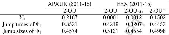
2-OU 2-OU 2-OU-I1 2-OU−

Y0 0.2167 0.0001 0.0012 0.1502

Jump times ofΦ1 0.3521 0.4219 0.3207 0.4452

Jump sizes ofΦ1 0.4574 0.5121 0.4554 0.4998

Table 5: Posterior predictivep-values for a range of models for the APXUK and EEX indices over the sample period January 24, 2011 to February 2, 2015.

the total number of jumps (of any size) per unit time is less than a third for the 2011-2015 data compared to 2001–2006.

From Table 5, the 2011-2015 EEX data in fact supports the 2-OU−model which has a single,

negative jump component (motivating the superscript minus in the notation). In this model the small number of larger upward price movements above the mean level in Figure 1 must therefore be accounted for by correspondingly large residuals in the diffusion component Y0, and this

explains the relatively low predictive p-value (0.1502) for Y0. With regard to the statistics of

the negative jump component, the valuesλ1, η1, β1 in Table 6 should be compared to the values

of λ2, η2, β2 in Table 4. Since negative prices were introduced in this market on September 1,

2008 (Genoese et al., 2010), in general larger negative jumps were possible in the 2011-2015 data. Indeed the most significant downward jump in 2011-2015 was to a large negative price, and our finding 0.593 = β₁New > β₂Old = 0.4308 is consistent with this change to the EEX market structure. For the diffusion component, the coefficientλ0 decreases from 11.9 and 8.22

for the APXUK and EEX markets respectively to approximately 3.6, a value which happens to be consistent across both markets.

5. Discussion

5.1. Scope of contribution

ACCEPTED MANUSCRIPT

APXUK (2011-15) EEX (2011-15)

2-OU model 2-OU−model

Parameter Mean SD Mean SD

µ 0.9865 0.0095 1.0480 0.0149

σ2 0.0071 0.0006 0.0170 0.0016

e−1/λ0 0.7537 0.0232 0.7590 0.0251

(λ0) (3.5727) (0.3976) (3.6736) (0.4526)

e−1/λ1 0.2104 0.0394 0.1941 0.0381

(λ1) (0.6435) (0.0781) (0.6115) (0.0741)

η1 0.1172 0.0324 0.1105 0.0310

β1 0.3981 0.0921 0.5930 0.1325

Table 6: Posterior properties obtained when calibrating the 2-OU (one positive jump component) and 2-OU−(one

negative jump component) models to the APXUK and EEX datasets respectively. The sample period is January 24, 2011 to February 16, 2015.

the real options framework (see for example Kitapbayev et al. (2015); Moriarty and Palczewski (2017)). In derivative pricing a main goal is to combine the latter models with observed derivative prices to construct so-calledrisk-neutralormartingaleprobability measures. Thus while model parameters are inferred from derivative prices it is important to identify the right class of price models, and our work provides an approach to this question via posterior predictive checking. In contrast, in real options analyses the fact that real projects are not traded means that the

physicalorhistoricprobability measure is often the one used. In this context our work provides an approach both to model specification and to the calibration of model parameters to historic data.

distri-ACCEPTED MANUSCRIPT

bution of the latent jump processes (blue, see Section A.3 for details) so that the agreement can be assessed.

5.2. Fundamental drivers

In this section we attempt to relate our empirical results to their underlying physical and eco-nomic drivers. Negative price spikes are associated with the priority given to wind energy in the spot market (Benth, 2013). A glut in wind power production can lead to a corresponding decrease in demand for other sources of generation. It can be impossible for conventional generators to reduce production sufficiently so they may temporarily accept low (or even negative) prices. In support of this analysis, we observed that the inclusion of a negative jump component was necessary for adequate modelling of the EEX data in both periods. Further the negative jumps had higher mean size in the later period, a change consistent with the increasing penetration of renewable generation.

While preprocessing the data we removed a deterministic seasonal component from the spot prices. However in some electricity markets (particularly in the US and Europe) seasonality has also been observed in the frequency of price spikes (Geman and Roncoroni, 2006; Benth et al., 2012). A priori this may be explained by greater levels of stress in the power system during the extremes of seasonal variation in weather due, for example, to heating load during cold snaps. The presence of jump seasonality was suggested in the 2000–2006 EEX data as illustrated in Figure 2, which displays the number of positive jumps on the EEX market by month, averaged over samples from our MCMC procedure. (It should be noted that Figure 2 is indicative and does not represent direct statistical estimates of jump frequency in spot prices.) Indeed for the latter series it was necessary to incorporate seasonality in the arrival rate of the positive jump component in order to obtain a statistically adequate model. In contrast seasonal jump components were not statistically necessary for the APXUK data in either period, which may be related to the less severe extremes of UK winter weather.

As presented in Section 4.2, there is statistical evidence for a reduction across both markets in both the number of positive jump components and the frequency of positive price spikes after the global financial crises of 2007-8 and 2009. It is true that in both the UK and Germany, electricity consumption generally increased in the period 2000–2006 and was generally level or decreased during 2011–2015.8 _{It follows that the power systems under study faced less stress}

from constraints in either production or transmission capacity during the latter period, and this is consistent with the observed reduction in positive price spikes. It must be noted however that