Wolfgang Schwanghart6 , Natalie S. Wolfenbarger2 , Kristen M. Thyng7 , David E. Gwyther8 , Alex S. Gardner1 , and Donald D. Blankenship2
1Jet Propulsion Laboratory, California Institute of Technology, Pasadena, CA, USA,2Institute for Geophysics, John A.
and Katherine G. Jackson School of Geosciences, University of Texas at Austin, Austin, TX, USA,3Department of Earth, Environmental, and Planetary Sciences, Brown University, Providence, RI, USA,4Joint Institute for the Study of the Atmosphere and Ocean (JISAO), University of Washington, Seattle, WA, USA,5NOAA Alaska Fisheries Science Center, Seattle, WA, USA,6Institute of Environmental Sciences and Geography, University of Potsdam, Potsdam, Germany, 7Department of Oceanography, Texas A&M University, College Station, TX, USA,8Institute for Marine and Antarctic
Studies, University of Tasmania, Hobart, Tasmania, Australia
Abstract
Climate science is highly interdisciplinary by nature, so understanding interactions between Earth processes inherently warrants the use of analytical software that can operate across the disciplines of Earth science. Toward this end, we present the Climate Data Toolbox for MATLAB, which contains more than 100 functions that span the major climate-related disciplines of Earth science. The toolbox enables streamlined, entirely scriptable workflows that are intuitive to write and easy to share. Included are functions to evaluate uncertainty, perform matrix operations, calculate climate indices, and generate common data displays. Documentation is presented pedagogically, with thorough explanations of how each function works and tutorials showing how the toolbox can be used to replicate results of published studies. As a well-tested, well-documented platform for interdisciplinary collaborations, the Climate Data Toolbox for MATLAB aims to reduce time spent writing low-level code, let researchers focus on physics rather than coding and encourage more efficacious code sharing.Plain Language Summary
This article describes a collection of computer code that has recently been released to help scientists analyze many types of Earth science data. The code in this toolbox makes it easy to investigate things like global warming, El Niño, or other major climate-related processes such as how winds affect ocean circulation. Although the toolbox was designed to be used by expert climate scientists, its instruction manual is well written, and beginners may be able to learn a great deal about coding and Earth science, simply by following along with the provided examples. The toolbox is intended to help scientists save time, help them ensure their analysis is accurate, and make it easy for other scientists to repeat the results of previous studies.1. Introduction
Scientific journals have recently been imposing more strict requirements for authors to share code along-side the publication of any scientific results. However, compliance rates remain low, and researchers still spend a great deal of time rewriting code that has been written before, deciphering whatever scant code is publicly available, or attempting to verify that their own basic analytical functions are in proper working order (Fecher et al., 2015; Greene & Thirumalai, 2019; Stodden et al., 2018).
To address some of the issues that may be preventing proper code sharing in our community (Acord & Harley, 2013; Barnes, 2010; Costello, 2009) and to provide a common framework for Earth science collab-orations to take place, we present the Climate Data Toolbox for MATLAB (CDT). The toolbox is intended primarily to enable efficient scientific research, but due to its thorough, pedagogically written documenta-tion, CDT may also serve as a learning tool for students and established researchers alike. CDT offers more than 100 fully documented MATLAB functions that span every step of scientific analysis, from data import to analysis to figure generation. As such, it enables fully scriptable, repeatable workflows that are intuitive to write and easy to share.
CDT is not the first numerical analysis toolbox to be geared toward the Earth sciences. Packages tailored to highly specialized applications abound in every major scientific computing language, and some efforts Key Points:
• We present a suite of MATLAB functions for efficient, scriptable analysis of Earth science data • The design of the toolbox is
interdisciplinary and process based • Pedagogical documentation serves as
a teaching tool while providing code validation
Correspondence to: C. A. Greene, [email protected]
Citation:
Greene, C. A., Thirumalai, K., Kearney, K. A., Delgado, J. M., Schwanghart, W., Wolfenbarger, N. S., et al. (2019). The climate data toolbox for MATLAB.Geochemistry, Geophysics, Geosystems,20. https:// doi.org/10.1029/2019GC008392
Received 17 APR 2019 Accepted 5 JUN 2019
Accepted article online 27 JUN 2019
have been aimed more generally at climate science. To name a few, the Climate Data Operator software offers a suite of tools for analyzing primarily NetCDF and GRIB data, and the now-defunct NCAR Com-mand Language was designed by climate scientists to meet a broad range of analytical and visualization needs. CLIMLAB (Rose, 2018) for Python is a well-documented toolbox created specifically for climate data analysis, and recently, the Python and Pangeo communities have been embracing operator packages such as pandas (McKinney, 2010) and xarray (Hoyer & Hamman, 2017) as efficient means of operating on climate data sets. CDT adds to the list of climate-related numerical packages in existence while taking advantage of the familiar syntax and unique design aspects of the MATLAB environment.
2. CDT Contents
CDT contains over 100 well-documented functions designed to help users at every step of scientific anal-ysis, from importing and processing data to plotting and interpreting results. The functions are intended to streamline workflows and ensure that users never feel stranded at any step of their analysis. Accord-ingly, the types of functions in CDT span the gamut from simple utilities, like one that returns the RGB color values corresponding to the name of any color, to functions for generalized statistical analysis, to discipline-specific functions such as one that calculates oceanographic mixed layer depths from ocean temperature measurements. Below, we outline the overall scope of CDT and highlight a few key functions.
2.1. Mathematics and Matrix Operations
Mathematics make up the basic tools of Earth science, but while MATLAB is adept at mathematical compu-tation, for many applications, it is not always apparent how to use standard MATLAB functions to operate on Earth science data sets.
For example, “data cubes” are common in Earth science, wherein a variable is stored in a 3-D matrix whose first two dimensions are spatial (such as longitude and latitude) and whose third dimension corresponds to time. Although a select number of MATLAB's built-in functions do allow users to specify a dimension of operation, many common operations such as detrending down the temporal dimension of a data cube may leave users bewildered. Faced with this task, most users opt to loop through each row and each column of the data cube, detrending each time series, one geographic grid cell at a time. For reference, this looping method applied to a somewhat coarse-resolution, quarter-degree global grid would require performing the operation more than one million times. Yet looping through each row and column of a data cube is the most intuitive option, so these kinds of nested loops are often employed despite their slow performance.
CDT offers a pair of functions calledcube2rectandrect2cube, which together make it intuitive and easy to reshape data cubes for efficient analyses. For the case of detrending a data cube, the user must only reshape it into a rectangular matrix withcube2rect, employ the standarddetrendfunction, and then reshape the detrended rectangular matrix back into a cube withrect2cube. The steps are intuitive, efficient, and endlessly adaptable as they bring into reach any standard MATLAB function that operates down columns of a 2-D matrix.
Thecube2rectandrect2cubefunctions can be called directly by users, but they are also called by several other CDT functions such as thetrendfunction, which efficiently calculates linear trends and uncertainties along any dimension of a matrix, or thewmeanfunction, which calculates weighted means. And in a similar way, the CDT functionscorr3,xcorr3, andxcov3usecube2rectandrect2cube
to obtain spatial patterns of relationships between a time series array and a gridded data cube.
In addition tocube2rectandrect2cube, CDT also offers alocalfunction, which simply provides a time series of local statistics within a masked region of interest. For example, a time series of a country's area-averaged surface temperature can be extracted from a temperature data cubeT, simply by defining a 2-D mask corresponding to the country's political boundaries. Just as easily, thelocalfunction can be used to extract a mean temperature profile as a function of depth for the Mediterranean Sea, given a 3-D oceanographic temperature data set and a 2-D mask defining the region of interest.
2.2. Earth-Science Functions 2.2.1. Seasonal Variability
have its mean and linear trend removed, and then means of the remaining anomalies may be calculated using the values corresponding to each day or month of the year. After establishing seasonal anomalies in this way, the matrix can then be permuted back into its original shape.
None of the steps of assessing a seasonal cycle are difficult per se using built-in MATLAB functions, but for someone who simply wishes to remove the seasonal cycle from a 3-D gridded sea surface temperature data set, the added steps of reshaping, detrending, and looping through each day or month of the year each introduce room for error while pulling attention away from the processes under investigation. Furthermore, it is quite possible that most users neglect to remove long-term trends before assessing seasonal variability.
CDT addresses the most common issues related to seasonal variability by providing aseasonfunction to assess the seasonal component of variability in a vector or data cube, adeseasonfunction to remove seasonal variability, and a climatologyfunction, which gives the seasonal component of variability while preserving the mean. In addition, asinefitfunction fits a sinusoid to seasonally varying data, and
sinefit_bootstrapprovides a measure of uncertainty for the fit.
2.2.2. Georeferenced Grids
The Earth is characterized not only by seasonal cycles but also by a general roundness in shape. That's not a terribly profound statement, but it has a profound impact on how we process most climatological data sets. Specifically, data sets whose grid cells are arranged on regular intervals of latitudes and longitudes are marked by increased spatial resolution near the poles. Accounting for the effect of shrinking grid cell areas with increasing distance from the equator is a common exercise in introductory climate science courses, but in practice, the process of looking up the formula for latitude-dependent grid cell areas is not time well spent, and it only introduces room for error.
CDT addresses the issue of grid cell areas with a function calledcdtarea, which, when paired withwmean, provides a straightforward way to obtain area-weighted means of gridded variables. Further, acdtdim
function gives the nominal dimensions of georeferenced grid cells and is called bycdtgradient, cdtdi-vergence, andcdtcurlto compute the changes in georeferenced scalar or vector fields relative to zonal and meridional distances along the Earth's surface.
2.2.3. Climate Indices
Several common metrics of climate variability are included in CDT. Among them, anensofunction fol-lows the method put forth by Trenberth (1997) to calculate the El Niño Southern Oscillation Index from sea surface temperatures, and anamofunction computes a version of the Atlantic Multidecadal Oscillation index (Enfield et al., 2001). Asamfunction follows the procedure laid out by Marshall (2003) to calculate the Southern Annular Mode from surface pressure data, and a similarnaofunction is provided for the North Atlantic Oscillation (Hurrell, 1995). For precipitation anomalies and drought assessment, apetfunction computes potential reference evapotranspiration following Hargreaves and Samani (1985), andspei pro-vides a standardized precipitation-evapotranspiration index following McMahon et al. (2013). While the present release of CDT includes functions for many of today's most commonly used climate indices, the toolbox is designed to allow inclusion of more such functions as demand dictates in the future.
2.2.4. Geophysical Attributes
In addition to functions that derive climate indices from measured or modeled quantities, CDT also contains several functions that describe inherent nominal properties of the Earth. Such functions includeisland, which bilinearly interpolates a 1/8◦mask data set to determine whether geographic locations correspond to present-day land or water. Similarly, thedist2coastfunction calculates distances to the nearest coastline, and thetopo_interpfunction interpolates topographic elevations from the 1/12◦ETOPO5 global grid (NGDC, 1993). Theair_pressureandair_densityfunctions compute the barometric formula for a U.S. Standard Atmosphere, and a suite of functions provide top-of-atmosphere radiation (as in McCullough, 1968; McMahon et al., 2013), daily insolation (as in Huybers, 2006), and solar angles for any given time, day, and location on Earth. Although researchers who study Earth surface processes may need a higher resolution data set than what is provided by thetopo_interpfunction and someone who studies complex atmospheric processes may wish for a more nuanced model than the U.S. Standard Atmosphere, the CDT functions provide basic geophysical attributes that will likely be of value as simple reference models that provide context in multidisciplinary studies.
2.3. Graphical Displays and Mapmaking
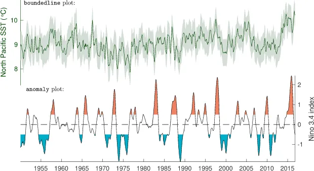
Figure 1.These tightly spaced plots were created with thesubsubplotfunction. The upper axes show a
boundedlineplot of sea surface temperature (SST) whose color was set asrgb(dark green), and the lower axes
show a shadedanomalyplot. The axes were labeled with thentitlefunction.
too far apart, it is unclear how to create a line plot with shaded error bounds, shaded anomaly plots are not supported, and only one colormap is supported in a given set of axes. To meet these needs, CDT offers over a dozen simple plotting functions, including asubsubplotfunction to enable tightly spaced subplots,
boundedlineto create line plots with shaded bounds,anomalyto create shaded anomaly plots, and
newcolorbar, which enables multiple color maps and color bars in the same set of axes. Examples are shown in Figure 1. CDT also introduces updates to the perceptually uniformcmoceancolor maps (Thyng et al., 2016), including new color maps designed specifically for precipitation totals, precipitation anomalies, and topographic relief.
For mapmaking, CDT extends the functionality of MATLAB's licensed Mapping Toolbox to enable more intuitive and powerful methods of displaying geospatial data. For example, political boundaries are easily added to Mapping Toolbox coordinates using thebordersmfunction, and regions of statistical significance are easily denoted using thestipplemfunction.
For users who do not have a license for the Mapping Toolbox or who desire the computational performance of plotting in unprojected coordinates, abordersfunction plots national boundaries using longitudes asx
values and latitudes asyvalues. Similarly, astipplefunction may be used to indicate regions of statistical significance, and apatschscfunction plots color-scaled patch objects on unprojected coordinates. If 3-D depictions of the Earth are desired, a suite of globe functions enable all the standard plotting capabilities but with the benefit that the globes may be manually rotated, allowing physically intuitive exploration of geospatial relationships.
2.4. Data-Format-Specific Functions
Some data formats that are commonly used in the geosciences present technical barriers when attempting to read or work with the data. In particular, NetCDF and HDF5 data sets can be read using standard MAT-LAB functions, but working with the data is often unwieldy. Converting dates to a usable form requires manual effort, and hierarchical data structures become cluttered in the MATLAB workspace. CDT alleviates minor headaches withncdateread, which automatically reads time data from NetCDF files that follow the standard Climate and Forecast metadata conventions, a converts the data into datetime format. The CDT functionsncstructandh5structread NetCDF and HDF5 data into tidy MATLAB structures. CDT also contains functions for working with other data-specific formats, such asxyzreadandxyz2gridto read grids generated by Generic Mapping Tools (Wessel et al., 2013) andbinind2latlonwhich allows straightforward processing of binned-index values from the type of sinusoidal grids employed by NASA's Ocean Biology Processing Group.
2.5. Tutorials
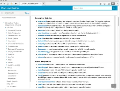
Figure 2.Complete, HTML-formatted documentation is viewable by typingcdtinto the Matlab Command Window.
To view the documentation for a specific function, follow thecdtcommand with the name of the function of interest.
For example, typecdt amoto view documentation for the Atlantic Multidecadal Oscillation function.
from insights that are not linked to a particular function but are more broad and inform decisions about which function is used. For example, displaying an effective and informative map of sea surface temperature anomalies requires understanding the strengths and weaknesses of the different types of maps that can be generated in MATLAB. Depending on the application, users may tolerate unprojected coordinates in exchange for the benefits of using standard plotting functions; they might want the projections and display options that come with using MATLAB's licensed Mapping Toolbox; they may prefer syntax and power of the M_Map Toolbox (Pawlowicz, 2018); or they may find that plotting on a globe best suits their purposes.
The decision about what type of map to generate comes before looking up function syntax, and many users may need help understanding the trade-offs of the different options to help them decide which map best suits their needs. For these cases, CDT offers tutorials, including a tutorial that lays out the major benefits and drawbacks of each type of map, and shows how an example climatological data set appears when displayed in each form.
The tutorials in CDT are part of a holistic approach to toolbox design (Greene & Thirumalai, 2019). This means considering not only how each function works on its own but also how the user will interact with the toolbox as a whole. It means meeting users where they are, not only in terms of the format of their raw data but also with an understanding of the decisions a user must make in the entire process of analyzing and displaying their data. Tutorials help fill in the gaps between functions while providing greater context to help users better understand their own work.
2.6. Sample Data Sets
primarily for use as example data in function documentation, where guided examples show users how to load and analyze realistic data and using CDT functions. The sample data sets can also provide convenient ground truth values that users can employ for context or for testing and documenting their own functions.
3. CDT Documentation
Thorough documentation is a principal characteristic of CDT. Each of the 100+ functions in CDT has a text header accessible by thehelpcommand, in which every acceptable combination of function syntax is listed and described. Syntax and Description sections also appear in HTML-formatted pages which are viewable in the MATLAB Documentation Browser (see Figure 2). Each HTML-formatted documentation file is designed to mimic standard MATLAB documentation, with an introductory paragraph, descriptions of function syntax, examples, and reference citations where appropriate.
3.1. Pedagogical Design
The overarching philosophy of CDT is that users should not experience any functional or conceptual gaps in standard workflows, from importing data to presenting results. This philosophy defined the overall scope of the toolbox, and it is seen throughout the function documentation. Anticipating gaps means recognizing that simple tasks such as importing NetCDF data into MATLAB might give novice users the sense of being stranded, without any idea where to begin. Accordingly, we provide a guide to importing NetCDF data, and we address other similar issues with tutorials, explanations, and links to resources where topics are covered in greater detail. Although we have attempted to accommodate beginners, we also recognize that most users will simply want to reference the documentation in search of quick reminders about function syntax, so we have made efforts to keep the elementary explanations brief or unobtrusive.
To benefit both novice and expert users, CDT documentation presents examples in full context. For exam-ple, thetopo_interpfunction shows how to interpolate topographic elevations to arbitrary geographic coordinates, beginning with an explanation of how to usecdtgridto simply create a quarter-degree global grid of geographic coordinates. After elevations are interpolated to the grid points, the documentation then shows how to apply an appropriate topographic color map using thecmoceanfunction. Another example describes how to use gridded topographic data to depict areas that are vulnerable to sea level rise. In this way, CDT follows Rose (2018) by seamlessly blending technical documentation and process-oriented tutorials.
Beyond simple examples and hypothetical scenarios of catastrophic sea level rise, CDT documentation also provides insights into the types of meaningful Earth-science processes that are actively under investigation in today's research institutions. We follow the philosophy of the Climate Data Guide (Schneider et al., 2013) by offering narrative guidance to users about the strengths and weaknesses of different methods of analyzing particular datasets. Throughout CDT's documentation, we explain not only how to perform each step of analysis but also why each step was performed and how to begin interpreting the results.
3.2. Real-World Examples
The documentation of CDT is written to ensure all examples feel tangible and are presented in proper con-text. The key to this approach includes real-world examples of climate data analysis, presented with detailed explanations of analytical procedures in the function documentation.
Wherever theoretical examples are warranted to establish the underlying principles of an analytical pro-cedure, function documentation begins with an overview of the theory. One such case is seen in the documentation for thetrendfunction, in which the user is shown how to generate a noisy array of pre-scribed slope andyintercept before applying thetrendfunction to assess the least-squares linear trend of the array. When the answer is inevitably close to the prescribed slope but does not match it exactly, we take the opportunity to point out that noise in the data can influence the value of the least-squares fit. The docu-mentation then goes on to explore the effect of noise on the statistical significance of calculated trends and briefly describes howpvalues are sometimes a useful metric. Only after the theory is well established do we load a data cube of sea surface temperatures to assess the distribution, magnitude, and statistical significance of the ocean warming that has been observed in recent decades.
serves to validate the CDT code while also supporting the results of previous work (Stodden et al., 2016). And finally, by mimicking published papers, CDT documentation serves as a teaching tool.
Just as novice guitarists develop their skills by looking up chords to their favorite songs, budding scientists should be given the opportunity to mimic the masters before being expected to add to the scientific canon. To this end, many of the CDT documentation files feature exact, step-by-step guides to recreating the results of previous studies.
In the documentation for theensofunction, for example, users are shown how to analyze sea surface tem-peratures with theensofunction and use theanomalyfunction to reproduce the main figure of the seminal work in which Trenberth (1997) defines El Niño. Similarly, theekmandocumentation recreates a map of wind-driven upwelling from Kessler (2002),mldmimics a plot of oceanic mixed layers by Holte and Talley (2009), and several other documentation files follow suit, recreating published work down to the color schemes and font styles of the original plots. In cases such as theeofdocumentation, where our empirical orthogonal function analysis of sea surface temperatures yields slightly different results from those pub-lished by Messié and Chavez (2011), we take the opportunity to discuss the likely causes of the discrepancy. By showing users how to apply CDT functions and helping them understand how to interpret results, CDT gives a head start to scientists and then ensures they begin heading in the right direction.
4. Conclusions
CDT is designed primarily for scientific analysis, but it is well enough documented that any graduate student could develop an intuition for the physical processes and analytical techniques that make up the building blocks of Earth science, simply by reading the documentation. As a toolbox, CDT is unique in that it is multidisciplinary, yet thoroughly and pedagogically documented. CDT provides technical on-ramps to help new users begin their analysis and conceptual bridges to link textbook theory to real data analysis.
The tools in CDT meet the needs of climate scientists at every stage of analysis, from importing and analyz-ing data to displayanalyz-ing results. The process-oriented functions help users keep their focus on physics rather than coding, and CDT syntax is simple, intuitive, and quick to learn. Analyses performed in CDT are fully scriptable and straightforward, which together, we hope will enable easy collaborations, an increase in code sharing, and a higher degree of replicablility for science as a whole.
References
Acord, S. K., & Harley, D. (2013). Credit, time, and personality: The human challenges to sharing scholarly work using Web 2.0.New Media & Society,15(3), 379–397.
Barnes, N. (2010). Publish your computer code: It is good enough.Nature News,467(7317), 753–753. Costello, M. J. (2009). Motivating online publication of data.BioScience,59(5), 418–427.
Dow, C. F., Lee, W. S., Greenbaum, J. S., Greene, C. A., Blankenship, D. D., Poinar, K., et al. (2018). Basal channels drive active surface hydrology and transverse ice shelf fracture.Science Advances,4(6), eaao7212. https://doi.org/10.1126/sciadv.aao7212
Enfield, D. B., Mestas-Nuñez, A. M., & Trimble, P. J. (2001). The Atlantic Multidecadal Oscillation and its relation to rainfall and river flows in the continental US.Geophysical Research Letters,28(10), 2077–2080.
Fecher, B., Friesike, S., & Hebing, M. (2015). What drives academic data sharing?PloS one,10(2), e0118053.
Greene, C. A. (2017). Drivers of change in East Antarctic ice shelves (Unpublished doctoral dissertation), The University of Texas at Austin. Greene, C. A., & Blankenship, D. D. (2018). A method of repeat photoclinometry for detecting kilometer-scale ice sheet surface evolution.
IEEE Transactions on Geoscience and Remote Sensing,56(4), 2074–2082. https://doi.org/10.1109/TGRS.2017.2773364
Greene, C. A., Blankenship, D. D., Gwyther, D. E., Silvano, A., & van Wijk, E. (2017). Wind causes Totten Ice Shelf melt and acceleration.
Science Advances,3, e1701681.
Greene, C. A., Gwyther, D. E., & Blankenship, D. D. (2017). Antarctic Mapping Tools for Matlab.Computers & Geosciences,104, 151–157. Greene, C. A., & Thirumalai, K. (2019). It's time to shift emphasis away from code sharing.Eos,100(5), 16–17. https://doi.org/10.1029/
2019EO116357
Greene, C. A., Thirumalai, K., Kearney, K. A., Delgado, J. M., Schwanghart, W., Wolfenbarger, N. S., et al. (2019). The Climate Data Toolbox for MATLAB.
Greene, C. A., Young, D. A., Gwyther, D. E., Galton-Fenzi, B. K., & Blankenship, D. D. (2018). Seasonal dynamics of Totten Ice Shelf controlled by sea ice buttressing.The Cryosphere,12(9), 2869–2882. https://doi.org/10.5194/tc-12-2869-2018
Hargreaves, G. H., & Samani, Z. A. (1985). Reference crop evapotranspiration from temperature.Applied Engineering in Agriculture,1(2), 96–99. https://doi.org/10.13031/2013.26773
Holte, J., & Talley, L. (2009). A new algorithm for finding mixed layer depths with applications to Argo data and Subantarctic Mode Water formation.Journal of Atmospheric and Oceanic Technology,26(9), 1920–1939. https://doi.org/10.1175/2009JTECHO543.1
Hoyer, S., & Hamman, J. (2017). xarray: N-D labeled arrays and datasets in Python.Journal of Open Research Software,5(1), 10. https:// doi.org/10.5334/jors.148
Hurrell, J. W. (1995). Decadal trends in the North Atlantic Oscillation: Regional temperatures and precipitation.Science,269(5224), 676–679.
Huybers, P. (2006). Early Pleistocene glacial cycles and the integrated summer insolation forcing.Science,313(5786), 508–511. https://doi. org/10.1126/science.1125249
Kessler, W. S. (2002). Mean three-dimensional circulation in the northeast tropical Pacific.Journal of Physical Oceanography,32(9), 2457–2471.
Marshall, G. J. (2003). Trends in the Southern Annular Mode from observations and reanalyses.Journal of Climate,16(24), 4134–4143. https://doi.org/10.1175/1520-0442(2003)016<4134:TITSAM>2.0.CO;2
McCullough, E. C. (1968). Total daily radiant energy available extraterrestrially as a harmonic series in the day of the year.Archiv für Meteorologie, Geophysik und Bioklimatologie, Serie B,16(2-3), 129–143. https://doi.org/10.1007/BF02243266
McKinney, W. (2010). Data structures for statistical computing in python. InProceedings of the 9th python in science conference(Vol. 445, pp. 51–56). Austin, TX.
McMahon, T. A., Peel, M. C., Lowe, L., Srikanthan, R., & McVicar, T. R. (2013). Estimating actual, potential, reference crop and pan evaporation using standard meteorological data: A pragmatic synthesis.Hydrology and Earth System Sciences,17(4), 1331–1363. https:// doi.org/10.5194/hess-17-1331-2013
Messié, M., & Chavez, F. (2011). Global modes of sea surface temperature variability in relation to regional climate indices.Journal of Climate,24(16), 4314–4331. https://doi.org/10.1175/2011JCLI3941.1
NGDC (1993). 5-minute gridded global relief data (ETOPO5). updated 2016.
Pawlowicz, R. (2018). M_Map: A mapping package for MATLAB. https://www.eoas.ubc.ca/~rich/map.html
Rose, B. E. (2018). CLIMLAB: A Python toolkit for interactive, processoriented climate modeling.Journal Open Source Software,3(24), 659. Schneider, D. P., Deser, C., Fasullo, J., & Trenberth, K. E. (2013). Climate data guide spurs discovery and understanding.Eos, Transactions
American Geophysical Union,94(13), 121–122.
Stodden, V., McNutt, M., Bailey, D. H., Deelman, E., Gil, Y., Hanson, B., et al. (2016). Enhancing reproducibility for computational methods.
Science,354(6317), 1240–1241.
Stodden, V., Seiler, J., & Ma, Z. (2018). An empirical analysis of journal policy effectiveness for computational reproducibility.Proceedings of the National Academy of Sciences,115(11), 2584–2589.
Thyng, K. M., Greene, C. A., Hetland, R. D., Zimmerle, H. M., & DiMarco, S. F. (2016). True colors of oceanography: Guidelines for effective and accurate colormap selection.Oceanography,29, 9–13.
Trenberth, K. E. (1997). The definition of El Niño. Bulletin of the American Meteorological Society, 78(12), 2771–2778. https://doi.org/10.1175/1520-0477(1997)078<2771:TDOENO>2.0.CO;2