Snow thickness pro
fi
ling on Antarctic sea ice with GPR
—
Rapid and accurate measurements with the potential
to upscale needles to a haystack
Andreas A. Pfaffhuber1 , Jan L. Lieser2 , and Christian Haas3
1
NGI, Perth, Western Australia, Australia,2ACE CRC and IMAS, University of Tasmania, Hobart, Tasmania, Australia,3AWI, Bremerhaven, Germany
Abstract
Snow thickness on sea ice is a largely undersampled parameter yet of importance for the sea ice mass balance and for satellite-based sea ice thickness estimates and thus our general understanding of global ice volume change. Traditional direct thickness measurements with meter sticks can provide accurate but only spot information, referred to as“needles”due to their pinpoint focus and information, while airborne and satellite remote sensing snow products, referred to as“the haystack,”have large uncertainties due to their scale. We demonstrate the remarkable accuracy and applicability of ground-penetrating radar (GPR) snow thickness measurements by comparing them with in situ meter stick data from twofield campaigns to Antarctica in late winter/early spring. The efficiency and millimeter-to-centimeter accuracy of GPR enables practitioners to acquire extensive, semiregional data with the potential to upscale needles to the haystack and to potentially calibrate satellite remote sensing products that we confirm to derive roughly 30% of the in situ thickness. Wefind the radar wave propagation velocity in snow to be rather constant (± 6%),encouraging regional snow thickness surveys. Snow thinner than 10 cm is under the detection limit with the off-the-shelf GPR setup utilized in our study.
Plain Language Summary
Snow on sea ice, especially on Antarctic sea ice, plays a significant role in climate analysis due to its contribution to the mass and volume balance of the cryosphere. The thickness of snow on sea ice is not known in full detail as it is hard to derive from satellite data. Based on an extensive data set from two Antarctic winter/spring expeditions, we show the efficiency and accuracy of ground-penetrating radar to map snow thickness on a semiregional scale. Such surveys could potentially be extended to larger scales and contribute to satellite snow thickness algorithm calibration schemes.1. Introduction
To put our work in context, we will briefly illustrate the climatological impacts of snow on sea ice and the consequent importance of snow thickness observations. We will discuss the opportunities and limitations with remote sensing snow thickness estimates, introduce the concept of ground-penetrating radar (GPR) snow thickness survey, and review prior experience.
1.1. The Importance of Snow on Sea Ice
Snow is a key feature of the polar climate system and plays an important role as a geophysical layer. Snow on sea ice profoundly controls surface albedo, influences the sea ice mass balance and heat exchange between the atmosphere and the ocean, and is an important contribution to the freshwater balance of the polar oceans [Sturm and Massom, 2017]. With respect to remote sensing, snow can obscure the ice surface both visually and electromagnetically and therefore complicates the retrieval of geophysical sea ice parameters from airborne and satellite instruments [see, e.g.,Lubin and Massom, 2006]. Knowledge of the depth and structure of snow on sea ice is crucial for correct interpretation of altimeter data when estimating sea ice thickness (and subsequent volume) [e.g.,Kurtz et al., 2013;Xie et al., 2013].
1.2. Snow Thickness Profiling With Ground-Penetrating Radar
Georadar or ground-penetrating radar (GPR) is a well-established geophysical method and has been used for terrestrial snow thickness mapping both ground based [e.g.,Godio and Rege, 2016] and airborne (Ulriksen
[1989] orMarchand et al. [2003]). Canadian researchers experimented with helicopter-based GPR to map snow thickness on Arctic sea ice in the late 1990s and early 2000s [e.g.,Lalumiere and Prinsenberg, 2009].
Geophysical Research Letters
RESEARCH LETTER
10.1002/2017GL074202
Key Points:
•In situ data from 17 sites in East and West Antarctica confirm
ground-based GPR snow thickness profiling feasibility on winter/spring sea ice
•Average accuracy of GPR-derived median snow thickness along 100 and 200 m long profiles is better than 1 cm
•Analysis of 1450 individual measurements results in a GPR snow thickness accuracy of 0.1 cm and 13.2 cm precision
Supporting Information:
•Supporting Information S1
Correspondence to:
A. A. Pfaffhuber, aap@ngi.no
Citation:
Pfaffhuber, A. A., J. L. Lieser, and C. Haas (2017), Snow thickness profiling on Antarctic sea ice with GPR—Rapid and accurate measurements with the potential to upscale needles to a hay-stack,Geophys. Res. Lett.,44, 7836–7844, doi:10.1002/2017GL074202.
Received 22 MAY 2017 Accepted 13 JUL 2017
Accepted article online 18 JUL 2017 Published online 14 AUG 2017
©2017. The Authors.
This is an open access article under the terms of the Creative Commons Attribution-NonCommercial-NoDerivs License, which permits use and distri-bution in any medium, provided the original work is properly cited, the use is
non-commercial and no modifications
Panzer et al. [2013] provide an overview on the performance of an airborne frequency-modulated continuous-wave radar that was successfully picking up internal snow layers as well as snow thickness on sea ice. However, they did not validate these radar snow thickness estimates with in situ measurements.
Newman et al. [2014] compared airborne snow thickness radar data with one ground-truth profile reporting good agreement for undeformed (level)first-year sea ice, within a few centimeters, and large differences over rougher surfaces underestimatingfirst-year ice snow by some 10% and overestimating multiyear ice snow thickness by around a factor of 3. The latter is attributed to surface roughness within the large footprint of airborne measurements, which reduces the coherence of reflected signals and limits the detection of clear radar scattering horizons. Radar results shown inNewman et al. [2014, Figures 3 and 8] are not as clear as the radargrams presented byPanzer et al. [2013] in terms of reflections stemming from the air/snow/ice inter-faces.Kwok and Maksym[2014] provide an extensive study of similar airborne radar snow thickness data acquired in Antarctica. Parts of their results were compared with in situ data revealing significant differences between radar and in situ thickness statistics, with radar overestimating by almost a factor of 2. These differ-ences were attributed to seasonal snow property effects, radar technology, and footprint limitations and dif-ferent sampling extent of the ground and airborne measurements. Thin snow is a challenge for airborne radars according to both ground truth studies (<8 cm [Kwok and Maksym, 2014] or<11 cm [Newman et al., 2014]).Pfaffling[2007] presents similar results based on GPR data acquired from a helicopter and with the antennas suspended from a ship crane; only thick and undeformed snow could be identified in the radargrams.
Here we present ground-based GPR snow-thickness data from two Antarctic late winter/early springfield campaigns, in East Antarctica (2003) and the western Weddell Sea (2006). Sampling locations are representa-tive of variousfirst-year ice and multiyear ice snow regimes occurring in the Southern Ocean. We compare the GPR results with extensive in situ data acquired with meter sticks and discuss the reasons for good agree-ment and uncertainties in detail. Additionally, and to illustrate the regional snow distribution at the survey times, we compare our data with an Advanced Microwave Scanning Radiometer–EOS (AMSR-E) snow thick-ness product [Cavalieri et al., 2014] and are able to confirm that earlierfindings of these retrievals underesti-mate in situ snow thickness [Worby et al., 2008]. Given the operational simplicity and rapid data acquisition, and at the same time high accuracy of GPR snow thickness profiling, this method may allow to close the missing scale between traditional spot measurements (needles) and large-scale airborne and satellite data estimates (the haystack).
2. Study Area
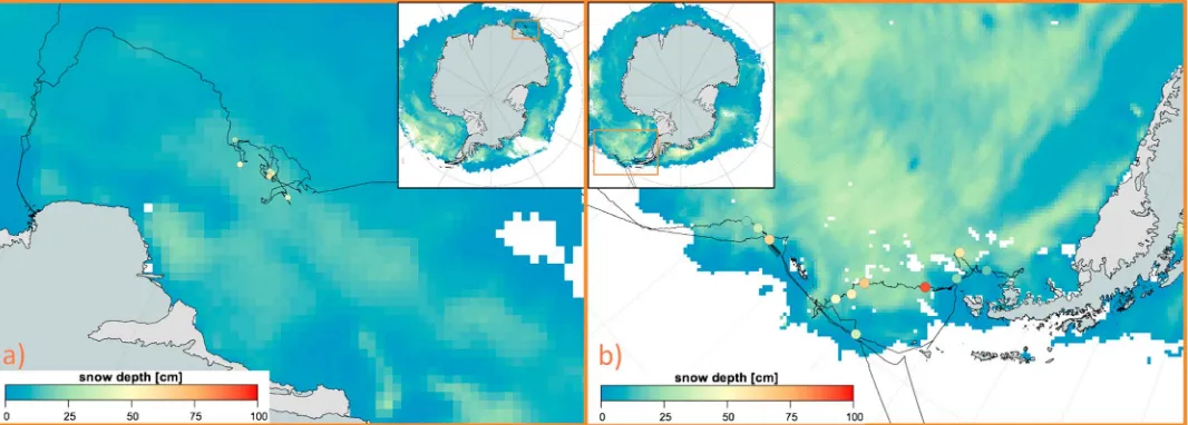
Massom et al. [2006] andLemke[2009] provide detailed reports from the expeditions, during which the data of this study were collected. Here we only briefly introduce study areas and the regional ice and snow conditions at the time (Figure 1).
2.1. The Antarctic Remote Ice Sensing Experiment 2003
The Antarctic Remote Ice Sensing Experiment (ARISE) was an Australia-led project aboard RSV Aurora Australis, in September/October 2003 in the East Antarctic. The experiment was designed to validate space-borne sea ice geophysical parameters such as concentration, deformation, and the thickness of snow on sea ice, with in situ observations covering 13 ship-based ice stations and 181 helicopter-based ministations [Massom et al., 2006]. It was set up infirst-year pack ice, south of the Antarctic Divergence. Ice conditions ranged from thin (less than 40 cm thick) levelfloes with a thin snow cover to thick highly deformedfirst-year
floes of 1 m to 2 m thickness and a deep snow cover dominated by drift. A detailed analysis of remote sensing snow thickness data compared to meter stick snow thickness and snow pit data collected during this project can be found inWorby et al. [2008]. The authors report a significant underestimation of snow thickness in the satellite data but a good agreement of remotely sensed sea ice concentration estimates and in situ data.
2.2. The Winter Weddell Outflow Study 2006
deformedfirst-year ice, and a region of relatively undeformed, youngerfirst-year ice in the west along the east coast of the Antarctic Peninsula. Extensive snow and ice thickness measurements were carried out by means of in situ sampling on individual icefloes and airborne surveying [Haas et al., 2009;Tan et al., 2012]. Typical snow plus ice thicknesses ranged from 0.1 m to 1.2 m off the Larsen B ice shelf to thicker than 0.8 m up to 2.5 m on some second-yearfloes. Meter stick snow thickness measurements were obtained on 25 icefloes, and on 12 of these sites, coincident GPR measurements were carried out. In addition, snow stratigraphy was measured in 12 snow pits. These showed the variable and partially highly metamorphous character of the snow in the northwestern Weddell Sea [Willmes et al., 2011].
3. Methods and Data
We are comparing snow thickness estimates by GPR and meter stick measurements and use a satellite pas-sive microwave product to illustrate the regional setting (Figure 1).
3.1. Meter Stick Snow Thickness
In situ, point measurements of snow thickness were performed by pushing a pointed meter stick vertically through the snow until it reached afirm interface (assumed to be the ice surface) and noting the ruler marking that aligns with the snow surface. Meter stick measurements are accurate to 1 to 2 cm, as the verti-cality is approximate, and the snow surface may not always be perfectly smooth. The majority of meter stick snow thickness measurements were acquired at 1 m spacing along 100 m or 200 m long profiles. A total of 1468 snow thickness values has been acquired this way. For detailed discussion on in situ snow thickness measurement techniques see, for example,Sturm[2009].
3.2. Ground-Penetrating Radar
The fundamentals of GPR, or georadar, can be studied in detail in various geophysical textbooks and publica-tions such asAnnan[2005] orKirsch[2006]. GPR instrumentation utilizes high-frequency electromagnetic waves, usually in the tens of megahertz to single digit gigahertz range that are sent into the ground as pulses or frequency sweeps [Kanagaratnam et al., 2007]. One or more receiver antennas record these waves for a
[image:3.612.42.575.92.283.2]finite time interval after the impulse has been sent. The recorded signals are visualized as radargrams (Figures 2a–2c) showing the intensity and travel time of the received signals. The emitted radar wave will reflect at interfaces with contrasting dielectric properties. Here we used two different off-the-shelf pulse radars: In 2003 we used a Mala RAMAC GPR with a shielded 800 MHz antenna [Otto, 2004]. In 2006, we used a GSSI SIR-3000 GPR unit with a shielded 400 MHz antenna [Pfaffling, 2007]. The nominal wavelength for these antenna frequencies is approximately 20 cm (800 MHz) to 40 cm (400 MHz). The theoretical (vertical) resolution of GPR data is typically quoted between ¼ and 1/30 of the radar wavelength and/or pulse length,
i.e., between 0.7 and 5 cm or 1.4 and 10 cm in air or roughly 1 and 6.5 cm or 1.8 and 13 cm in snow for the 800 MHz and 400 MHz antennas, respectively. Overall, these theoretical resolution estimates are from a few centimeters to around 10 cm with significant overlap.
The radar antennas were placed onto the bottom of a nonmetallic sledge and man dragged over the snow surface; therefore, the primary radar reflections originated from the snow/ice interface. With a known radar wave velocity, these radargrams can be directly translated to snow thickness readings (Figure 2c). Note that operating the radar antennas on the snow surface strongly reduces the radar footprint size compared to airborne measurements. As afirst approximation, derived from thefirst Fresnel zone, one can assume that the footprint has the same magnitude as the measured snow thickness for ground borne and the antenna altitude over ground for airborne radar measurements. Therefore, stronger and more coherent reflections can be received, improving the retrieval of travel times of individual radar traces as well as correlations between adjacent traces.
In terms of achievable snow thickness accuracy we must consider the signal sampling, rather than wave-length, because with a ground-based GPR there is no reflection from the snow surface. Therefore, we do not have to distinguish two individual reflections but can rather just locate the snow/ice reflection as accu-rately as possible. In 2006, a range window of 50 ns was recorded with 1024 samples leading to 0.05 ns/sam-ple or 1.2 cm/samns/sam-ple using 24 cm/ns as radar velocity. The best-case achievable snow thickness accuracy is thus in the centimeter range.
[image:4.612.34.578.91.355.2]To enhance the clarity of the snow/ice reflection, we applied standard practice processing steps to our radar data that are described in detail inPfaffling[2007] andOtto[2004] using the Reflexw (www.sandmeier-geo.de) software package. Briefly summarized for the 2006 data, preprocessing included georeferencing, declipping, and move of start time followed by batched 2-D processing consisting of background removal, dynamic correction, and autopicking of snow/ice reflections. The 2003 data processing included a band pass, direct current shift, and commonly declipping in addition to the steps described for 2006. To georeference the data, markers were set during acquisition at 10 m profile markers; these markers are then used to stretch or com-press the profile. In most cases the instrument’s autogain function prevented saturation and declipping was only necessary for some profiles.
Figure 2.Typical snow thickness radar results showing data from 28 September 2006 (a) raw unprocessed radargram, (b) radargram after 2-D processing, (c) picked
snow/ice reflections (black) superposed with meter stick depth measurements (green) and snow thickness histograms of radar data (red) and direct readings (white)
To simplify the later reflection picking, thefirst negative maximum of the direct wave was used to adjust the start time with respect to the 15 cm GSSI antenna spacing. Radar wave velocity was usually determined with direct measurements, by placing the GPR unit over a level snow patch with known thickness. Further 2-D processing was carried out as a batch job. First, a background removal was applied to remove the direct wave and potential further stationary ringing. This step is crucial to resolve thin snow 10 to 20 cm thick (Figure 2b). The start time is shifted by 0.5 ns to account for the negative peak in the preprocessing. Then dynamic correction is applied to account for the exact geometry between transmitter—reflector—receivers, in a sense that the data are reduced to common shot point. Now another time shift is applied to account for the thick-ness of the sledge bottom. The travel time is corrected from“snow plus sledge”to“snow.”
Finally, the snow/ice reflection is picked using automatic picking followed by careful manual evaluation and correction. Such corrections are needed when the automatic algorithm tracks reflections that clearly are not the snow/ice interface. This reflection is usually dominant and easy to spot for an interpreter (Figure 2b). Final quality control is to visualize meterstick readings with GPR picks (Figure 2c) before thefinal snow thickness histograms are being produced (Figures 2d and 2e). Snow thickness profiles are exported with a 10 cm mea-surement spacing leading to a total of 17.579 meamea-surement points (versus 1.468 meter stick readings at 1 and 2 m spacing). The GPR snow thickness profile is spatially downsampled to 10 cm to create an equidistant data set for reliable statistical analysis.
3.3. Passive Microwave Radiometer Snow Thickness
Snow cover parameters are available from spaceborne passive microwave data since the 1980s [Künzi et al., 1982], and we are using these estimates to provide a regional overview of snow conditions at the time of the twofield campaigns (Figure 1). A more detailed description of the snow thickness retrieval algorithm on Antarctic sea ice can be found inMarkus and Cavalieri[1998]. Note that this algorithm is based on similar meter stick measurements as presented here and would benefit from an inclusion of more extensive GPR data to increase reliability of results. Here we use data from the Advanced Microwave Scanning Radiometer–EOS (AMSR-E) publicly available via the U.S. National Snow and Ice Data Center [Cavalieri et al., 2014]. Among the snow science community, it is common knowledge that the AMSR-E algorithm underesti-mates in situ observations under Antarctic conditions [e.g.,Worby et al., 2008]. To assess this assumption, we analyzed AMSR-E snow depths for all sample days in our study (Table S1 in the supporting information),fi nd-ing little temporal variation durnd-ing each experiment. A linearfit through zero of median GPR versus AMSR-E snow thickness (Figure S1) confirms pervious findings, an approximately 30% underestimation of the observed in situ snow thickness.
4. Results
The aim of this work is to investigate the consistency of snow thickness estimates derived by direct, geophy-sical, and to some extent remote sensing methods. Each method has intrinsic uncertainties and limitations, and the key value for snow and sea ice science is their successful integration. In the following we show step by step how the various results intercompare and consequently may be up scaled from point measurements (needles) to polar coverage (the haystack).
4.1. Radar Propagation in Snow: From Radargram to Snow Thickness Distribution
To compute snow thickness from radar wave travel times, the speed of light in snow, i.e., the radar wave velo-city, which depends on the snow’s dielectric permittivity, must be known (as discussed in section 3.2). The dielectric permittivity of snow is governed by its density and wetness distribution. During the 2006field campaign, these parameters were measured in various snow pits [Haas et al., 2009] using a“snow fork,”a dielectric resonator, which records the dielectric permittivity directly [Sihvola and Tiuri, 1986;Nicolaus et al., 2009]. The dielectric properties were found to vary little with a mean permittivity of 1.55 ± 0.1.
With an average of 1.55 ± 0.1 as a typical Antarctic snow dielectric permittivity, the resulting radar velocities vary from 23 to 25 cm/ns, corresponding to a precision of ±3 cm for 80 cm thick snow. Note that this is not the actual accuracy of GPR snow thickness estimates (as discussed in section 4.2) but is the level of precision that can be expected with unknown dielectric permittivity. This means that also without a prior knowledge of the snow properties on thefloe sampled, GPR can retrieve high-quality snow thickness estimates, assuming a wave speed of ~24 cm/ns (assuming that a bias is to be expected for very thick and thin snow). It is also important to again note that these results are based on late winter/early spring condition; ourfindings may not apply for warmer spring/autumn snow with higher moisture content and consequently different dielectric properties.
The picked snow/ice reflection from the processed GPR data (as discussed in section 2) was migrated to depth estimates with the wave velocities determined above, and these snow thickness profiles were conse-quently binned in 2 cm and 5 cm histograms (Figures 2d and 2e). Median snow thickness and the corresponding standard deviation that form the basis of the further validation are given in Table S1.
4.2. Validation With Meter Stick Measurements
We derived median snow thickness estimates and standard deviations from both meter stick data and GPR data (Table S1) to study their mutual correlation (Figure 3a). The GPR-derived snow thickness readings have one fundamental limitation when it comes to very thin snow (less than 10 cm thick); that is, in these cases, the reflection from the snow/ice interface overlaps with the direct wave traveling from the transmit-ter to the receiver antenna. For snow thickness distributions with a significant presence of thin snow (under 10 cm thick), the GPR data will result in a higher median than the in situ data (Figure 4a and Table S1). This is the case for the three icefloes with the thinnest snow (Figure 3a). While the example in Figure 3a may suggest that also the 10–20 cm thickness interval is mispresented by the GPR data, we generallyfind 10 cm to be the actual detection limit. The histograms from the other sites with thin snow support this [Pfaffling, 2007].
[image:6.612.177.572.90.285.2]The mean difference between GPR and meter stick median snow thickness (Figure 3a) is 9.7 mm (RMS = 2.8 cm) including the deviating thin snow samples. The accuracy for snow thicker than 20 cm only is 1 mm (RMS = 1.3 cm). As 1 mm is beyond the uncertainty of the actual meter stick measurements we consider the GPR snow thickness results as a perfectfit to meter stick control data. Linear regression of the complete median data set results in anR2 of 0.981 and Zs_GPR = 1.011 Zs_in situ; excluding the three samples with snow thickness less than 20 cm leads toR2= 0.994 and Zs_GPR = 1.001 Zs_in situ. To further
Figure 3.Comparison of meter stick (Zs_in situ) with GPR results (Zs_GPR). (a) Meter stick and GPR measurements are
shown as mean thickness with standard deviation (error bars) and were derived from 100 m and 200 m long profiles.
(b) The complete 2006 data (1468 samples) are further shown as an individual scatterplot. Red bars in Figure 3a indicate the difference between GPR and meter stick median thicknesses. The red histogram in Figure 3b represents the deviation
analyze the correlation and accuracy of GPR snow thickness, we show all 1468 data points from the 2006 campaign and their deviation (ΔZs = Zs_GPR–Zs_in situ; Figure 3b). A linearfit of the individual data pairs results in anR2of 0.949 and Zs_GPR = 1.027 Zs_in situ. We also analyze the deviation between the GPR and in situ data (histogram in Figure 3b) resulting in a median of 0.1 cm and standard deviation of 13.2 cm. TheΔZs histogram with 1 cm bins peaks at the 0 interval.
4.3. The Potential for Upscaling to Regional Snow Thickness Estimates
In the previous sections we have discussed the match between AMSR-E, GPR, and meter stick snow thickness based on the small scale of 100 m to 200 m long profiles. For a 200 m profile the gain in efficiency using GPR instead of meter sticks is limited. The significance of such short profiles is, however, questionable when regio-nal data are needed to understand ice and snow processes. Short profiles represent only a very small sample and provide limited statistical significance. With GPR it is easily possible to achieve profile lengths of several kilometers within less than an hour. To illustrate the gained value with GPR, we present snow thickness his-tograms acquired on the same icefloe along a 200 m profile (Figure 4b) and along a 2.5 km long round track (Figure 4c). The round track covers the icefloe in“random walk”and is intended to provide a much more sta-tistically significant sample of the snow conditions than a short 200 m profile. Acquiring data along several kilometer-long profiles may establish an in situ snow thickness database that can be compared to remote sensing footprints. While the 200 m segment covers 2000 radar traces, the round track includes 136,000 data points. The thickness histograms clearly show the dominance of thick snow with a median thickness of 72 cm on the larger scale, while the 200 m profile is characterized by thinner snow not representative of the wholefloe.
5. Conclusions
We have shown that off the shelf, high-frequency (400–800 MHz) impulse radars are very capable of deriving the thickness of snow on sea ice. Our study found that dielectric permittivity was nearly constant in late winter/early spring (varying not more than ± 6%), allowing reliable migration from two-way travel times to snow thickness estimates. When comparing radar with meter stick data, the individual accuracy is in the centimeter range for almost all sites. Snow thickness histograms can get skewed when there are areas with very thin (<10 cm) snow as these are not resolvable by the GPR. To our knowledge, this is the most extensive validation of GPR snow thickness measurements on sea ice so far and our results agree withfindings of groups that have published both unvalidated regional data and validated local data.
[image:7.612.42.574.90.219.2]Based on ourfindings, GPR measurements are as accurate but more efficient and provide higher spatial reso-lution than traditional or automated meter sticks. We propose that GPR measurements can extend snow thickness survey extent by a factor of 10 or more. Thus, making purpose-developed, complicated step frequency/frequency-modulated radars is not strictly necessary for the task. The efficiency of GPR-based snow thickness profiling and mapping unlocks the opportunity offloe- or large-scale coverage, estimated to be large enough to upscale the historic in situ“needle”data to today’s rather qualitative remote sensing
Figure 4.Snow thickness histograms (5 cm bins) showing data from (a) 2 and (b, c) 12 October 2006 (cf. Table S1). Radar data in red and direct readings in black. In
Figure 4a parts of the profile were thinner than the GPR detection limit (10 cm), while Figures 4b and 4c show results from the samefloe based on Figure 4b a 200 m
profile and Figure 4c a 2.5 km profile. Vertical, thin lines show the respective median thickness; in Figure 4c the median from Figure 4b is included in black as a
“haystack”scales, as long as a sufficient number of icefloes can be sampled. This is particularly attractive for Antarctic sea ice with its generally thick snow cover. The necessary processing of radar data is minor and more efficient than digitizing hundreds of meter stick readings. Automatic snow depth probes may provide comparablefield efficiency yet still at lower data density than a continuous GPR profile. Key limitation remains physical access to icefloes by virtue of icebreaker, snowmobile, or aircraft to carry out ground work. Due to the larger footprint and need to detect both surface and bottom snow reflections, specialized, purpose-developed sensors remain necessary for airborne snow thickness radar mapping. However, ourfi nd-ings, with respect to near-constant radar velocity in the snow pack, however, encourage airborne snow thick-ness radar surveys to be undertaken when coincident dielectric snow properties cannot be measured. All the discussed data represent late winter/early spring conditions, and one must assume that snow properties would change later in the season.
The thickness of snow on sea ice is a crucial parameter to calibrate altimeter-based remote sensing sea ice products, yet no quantitative remote sensing sea ice products are available as of today. Regional GPR-based snow thickness data may provide the necessary calibration/correction of these crucial remote sensing esti-mates. The observed near-constant radar velocity motivates GPR surveys with very limited need for in situ calibration. As with any geophysical survey, GPR results should be used to locate sparse direct measurements, in this case, at areas with especially thin and thick snow.
References
Annan, A. P. (2005), Ground-penetrating radar in near-surface geophysics, pp. 357–438.
Cavalieri, D. J., T. Markus, and J. C. Comiso (2014), AMSR-E/Aqua Daily L3 12.5 km Brightness Temperature, Sea Ice Concentration, & Snow Depth Polar Grids, Version 3. [Antarcticfive-day snow depth over sea ice], NASA Natl. Snow and Ice Data Cent. Cent., Boulder, Colo., doi:10.5067/AMSR-E/AE_SI12.003.
Godio, A., and R. B. Rege (2016), Analysis of georadar data to estimate the snow depth distribution,J. Appl. Geophys.,129, 92–100, doi:10.1016/j.jappgeo.2016.03.036.
Haas, C., A. Friedrich, Z. Li, M. Nicolaus, A. Pfaffling, and T. Toyota (2009), Regional variability of sea ice properties and thickness in the northwestern Weddell Sea obtained by in-situ and satellite measurements, inThe Expedition of the Research Vessel“Polarstern”to the Antarctic in 2006 (ANT-XXX III/7),Rep.Polar Mar.Res, vol. 586, edited by P. Lemke, pp. 36–74, Alfred Wegener Inst. for Polar and Mar. Res, Bremerhaven, Germany.
Kanagaratnam, P., T. Markus, V. Lytle, B. Heavey, P. Jansen, G. Prescott, and S. P. Gogineni (2007), Ultrawideband radar measurements of thickness of snow over sea ice,IEEE Trans. Geosci. Remote Sens.,45(9), 2715–2724.
Kirsch, R. (2006), Groundwater geophysics.
Kurtz, N. T., S. L. Farrell, M. Studinger, N. Galin, J. P. Harbeck, R. Lindsay, V. D. Onana, B. Panzer, and J. G. Sonntag (2013), Sea ice thickness, freeboard, and snow depth products from Operation IceBridge airborne data,Cryosphere,7(4), 1035–1056.
Künzi, K. F., S. Patil, and H. Rott (1982), Snow-cover parameters retrieved from Nimbus-7 Scanning Multichannel Microwave Radiometer (SMMR) Data,IEEE Trans. Geosci. Remote Sens.,GE-20(4), 452–467.
Kwok, R., and T. Maksym (2014), Snow depth of the Weddell and Bellingshausen sea ice covers from IceBridge surveys in 2010 and 2011: An examination,J. Geophys. Res. Oceans,119, 4141–4167, doi:10.1002/2014JC009943.
Lalumiere, L., and S. Prinsenberg (2009), Integration of a helicopter-based ground penetrating radar (GPR) with a laser, video and GPS system, paper presented at 19th International Offshore and Polar Engineering Conference, Osaka, Japan.
Lemke, P. (2009), The expedition of the research vessel "Polarstern" to the Antarctic in 2006 (ANT-XXIII/7),Reports on Polar and Marine Research, 586, AWI, Bremerhaven, Germany.
Lubin, D., and R. A. Massom (2006),Polar Remote Sensing Volume 1: Atmosphere and Ocean, Springer, Chichester, U. K.
Marchand, W.-D., Å. Killingtveit, P. Wilen, and P. Wikström (2003), Comparison of ground-based and airborne snow depth measurements with Georadar systems, case study,Nord. Hydrol.,34(5), 427–448, doi:10.2166/nh.2003.025.
Markus, T., and D. J. Cavalieri (1998), Snow depth distribution over sea ice in the Southern Ocean from satellite passive microwave data, in
Antarctic Sea ice: Physical Processes, Interactions and Variability, edited by M. O. Jeffries, pp. 19–39, AGU, Washington, D. C.
Massom, R. A., et al. (2006), ARISE (Antarctic Remote Ice Sensing Experiment) in the East 2003: Validation of satellite-derived sea-ice data products,Ann. Glaciol.,44, 288–296.
Newman, T., S. L. Farrell, J. Richter-Menge, L. N. Connor, N. T. Kurtz, B. C. Elder, and D. McAdoo (2014), Assessment of radar-derived snow depth over Arctic sea ice,J. Geophys. Res. Oceans,119, 8578–8602.
Nicolaus, M., C. Haas, and S. Willmes (2009), Evolution offirst- and second-year snow properties on sea ice in the Weddell Sea during spring-summer transition,J. Geophys. Res.,114, D17109, doi:10.1029/2008JD011227.
Otto, D. (2004), Validation of GPR sea-ice- and snow-thickness measurements onfirst-year and multi-year sea-ice in the Arctic and Antarctic. (in German). Diploma Thesis, Technische Universität Clausthal.
Panzer, B., D. Gomez-Garcia, C. Leuschen, J. Paden, F. Rodriguez-Morales, A. Patel, T. Markus, B. Holt, and P. Gogineni (2013), An ultra-wideband, microwave radar for measuring snow thickness on sea ice and mapping near-surface internal layers in polarfirn,J. Glaciol.,
59(214), 244–254.
Pfaffling, A. (2007), Ground penetrating radar snow thickness profiling during WWOS 06—Field data report, Hamburg, Germany, doi:10.13140/RG.2.2.29249.76647.
Sihvola, A., and M. Tiuri (1986), Snow fork forfield determination of the density and wetness profiles of a snow pack,IEEE Trans. Geosci. Remote Sens.,GE-24(5), 717–721.
Sturm, M. (2009), Field techniques for snow observations on sea ice, inField Techniques for Sea Ice Research, edited by H. Eicken et al., pp. 25–49, Alaska University Press, Fairbanks, Alaska.
Acknowledgments
A.A.P. was an AWI employee in 2003 and a consultant to AWI in 2006. He is grateful to the NGI sabbatical fund that
Sturm, M., and R. A. Massom (2017), Snow in the sea ice system: Friend or foe?, inSea Ice, edited by D. N. Thomas, pp. 65–109, John Wiley & Sons Ltd., Chichester, U. K.
Tan, B., Z. J. Li, P. Lu, C. Haas, and M. Nicolaus (2012), Morphology of sea ice pressure ridges in the northwestern Weddell Sea in winter,
J. Geophys. Res.,117, C06024, doi:10.1029/2011JC007800.
Ulriksen, P. (1989), Radar measurements of equivalent water content in snow, measured from a helicopter, paper presented at EARSeL workshops and symposium, Helsinki Univ. of Technology, Espoo, Finland.
Willmes, S., C. Haas, and M. Nicolaus (2011), High radar-backscatter regions on Antarctic sea-ice and their relation to sea-ice and snow properties and meteorological conditions,Int. J. Remote Sens.,32(14), 3967–3984, doi:10.1080/01431161003801344.
Worby, A. P., T. Markus, A. D. Steer, V. I. Lytle, and R. A. Massom (2008), Evaluation of AMSR-E snow depth product over East Antarctic sea ice using in situ measurements and aerial photography,J. Geophys. Res.,113, C05S94, doi:10.1029/2007JC004181.