MoL 2014 14: An Automata Theoretic Perspective on Polyadic Quantification in Natural Language

(1)

An Automata-Theoretic Perspective on Polyadic

Quantification in Natural Language

MSc Thesis

(Afstudeerscriptie)

written by

Sarah McWhirter

(born October 11, 1989 in San Antonio, Texas)

under the supervision of Dr Jakub Szymanik, and submitted to the Board of Examiners in partial fulfillment of the requirements for the degree of

MSc in Logic

at theUniversiteit van Amsterdam.

Date of the public defense: Members of the Thesis Committee: July 2, 2014 Dr Maria Aloni

Prof. dr Johan van Benthem Dr Paul Dekker

(2)

Abstract

As part of the general project of procedural semantics, nearly thirty years ago van Benthem first proposed semantic automata as a computational model of natural language quantification. While automata-theoretic characterization re-sults have been obtained for monadic quantifiers, very little has been done to investigate polyadic quantifiers from this perspective. Polyadic quantification in natural language includes but is not limited to iteration, cumulation, resump-tion, reciprocals, and branching. A natural extension of the semantic automata model is to study the properties of automata recognizing polyadic quantifiers, and the operations on simple automata corresponding to the lifts giving rise to them.

(3)

Introduction

1.1 Motivations and Contributions

Nearly thirty years ago, van Benthem first introduced the notion of semantic automata, uniting generalized quantifier (GQ) theory and formal language the-ory in an elegant and powerful way. The basic idea is to use insights of GQ theory to identify a natural language quantifier with an automaton that, in a precise sense, recognizes the models in which it is true, letting us consider the quantifier as a procedure for checking whether it holds. This marriage enables the use of the Chomsky hierarchy as a measure of complexity of quantifiers, which “turns out to make eminent sense, both in its coarse and fine structure” [4]. Semantic automata have not only led to many observations interesting in their own theoretical right, but also to myriad insights in cognitive modeling and formal learning based on the idea of meaning as algorithm, as van Benthem himself predicted:

. . .the procedural perspective may also be viewed as a way of extending contemporary concerns in ‘computational linguistics’ to the area of semantics as well. Complexity and computability, with their background questions ofrecognition andlearning, seem just as relevant to semantic understanding as they do to syntactic parsing [4].

(6)

obtain stronger automata characterizations for some polyadic quantifiers? This thesis is inspired by a very recent (2013) answer to that question by Steinert-Threlkeld and Icard III [46], exploring semantic automata for iterated quanti-fiers. They show regular and context-free quantifier languages are closed under iteration; however, their proposed computational model is unnecessarily power-ful.

Also in 2013, Kanazawa [27] answered an open question in [38] characterizing the class of quantifiers recognized by deterministic pushdown automata by their corresponding semilinear sets. As it turns out, it is rather difficult to form simple natural language quantifiers that go beyond this characterization. Given this new result, it is interesting to ask whether this natural subset of context-free languages is closed under quantifier iteration.

Our first main contribution is a different construction of iteration automata that is appropriately powerful, which was admittedly missing from the semantic automata landscape thus far. Further, we extend iteration automata (both our version and that presented in [46]) to accomodate any number of quantifiers. Second, we prove that deterministic context-free languages are closed under iteration. The thesis also includes constructions for cumulation automata (for any number of regular quantifiers) and iterations in which one or more quantifier is deterministic context-free but non-regular.

Iterated quantifiers are definable in terms of their monadic constituents and constitute a sort of default for producing complex quantifiers. TheFrege bound-arydelineates just how much of polyadic quantification is attainable by multiple iterations, and there are indeed many natural language quantifiers beyond the boundary. Our final contribution is a first step toward establishing a correlate of the Frege boundary within the Chomsky hierarchy using the semantic automata framework.

We hope these contributions add momentum to the recent revival of interest in semantic automata, spurring further research into automata for polyadic quantifiers, and that the fruits of the algorithmic perspective on meaning may be brought to bear on practical applications related to multiquantifier constructions in natural language.

1.2 Themes

(7)

semantics of algorithmic meaning, considerations of complexity and determin-ism in natural language, the division between production and recognition in language understanding, compositionality, and the importance of representa-tions.

1.2.1 Meaning as Algorithm

The idea of meaning as algorithm may be traced all the way back to Frege [16] and his notion of Sinn: the meaning of an expression is the manner in which its reference is determined. This notion lives on in computational semantics in the idea that the meaning of an expression is analgorithm orprocedure for determining its extension in a model. This idea was first seriously formalized in Tichy’s Intension in terms of Turing machines [55], an “attempt to base semantics directly on the concept of sense.” Various possibilities for procedural semantics are discussed by van Benthem inTowards a computational semantics [5], including the semantic automata models for quantifiers that we further develop in this thesis.1

One of the biggest motivations to develop procedural semantics is the possibility of a psychologically plausible model of language. For example, Suppes claims:

The basic and fundamental psychological point is that, with rare exception, in applying a predicate to an object or judging that a re-lation holds between two or more objects, we do not consider prop-erties or relations as sets. We do not even consider them as somehow simply intensional properties, but we have procedures that compute their values for the object in question [47].

In cognitive science, Marr [33] has famously proposed that information process-ing systems, like the cognitive procedures employed in comprehendprocess-ing language, must be understood at three levels:

• Computational Theory (Level 1): What is the goal, why is it appropriate, and what is the logic of the strategy to carry it out?

• Representation and Algorithm (Level 2): How can the computational the-ory be implemented? How are the input and output represented, and how is one transformed into the other?

• Implementation (Level 3): How can the representation and algorithm be realized in a physical system?

Marr further claims that the highest level, the computational level, tells us most about the problem at hand, offering that “Trying to understand perception by studying only neurons is like trying to understand bird flight by studying only feathers.” We need first, for example, an understanding of aerodynamics to understand why bird feathers are particularly good for flying. The nature of

(8)

flight constrains the kind of mechanism that may implement flight, but plenty of (in)animate things fly without feathers. The same goes for a cognitive task like verifying the truth of a quantified sentence.

The approach in this thesis perhaps straddles the computational and algorith-mic level. Complexity differences between automata classes are reflected in measures of task difficulty, and even the more fine-grained structure of particu-lar automata lead to accurate empirical hypotheses; however, we do not claim that peopleactuallyimplement the algorithm represented by a given automata. Rather, semantic automata are idealized models of quantifier verification.2

Peo-ple may guess, approximate, or use some other strategy that is dependent upon the way the information is presented.

Steinert-Threlkeld puts it nicely:

In principle, they [semantic automata] allow for a separation be-tween abstract control structure involved in quantifier verification and innumerable other variables that the framework leaves under-specified . . .This could be viewed as a modest distinction between competence andperformance for quantifier expressions [46].

. . .the standard model-theoretic semantics of quantification could be seen as a potential computational, or level 1, theory. Semantic automata offer more detail about processing, but. . .less than one would expect by a full algorithmic story about processing (level 2), which would include details about order, time, salience, etc. Thus, we might see the semantic automata framework as aimed at level 1.5 explanation, in between levels 1 and 2, providing a potential bridge between abstract model theory and concrete processing details [46].

We discuss the fruitfulness of the semantic automata model in various practical applications in Section 9.1.

1.2.2 Determinism

If we pursue the paradigm of procedural semantics for its promise of the pos-sibility of a cognitively tenable model of language processing, we might attend to this goal from the get-go bynot positingimplausible models. Since we deal with machine characterizations of procedures in this thesis, we may look to the divide between determinism and non-determinism for at least one distinction between the plausible and implausible3_{. Non-deterministic automata simply do}

not provide realistic algorithmic models as they are not implementable. Even

2_{However, see [13] for the first step toward realistic semantic automata, using probabilistic}

transitions to model verification error.

3_{Dealing with computational complexity, Szymanik [50] takes}_tractability _{as the natural}

notion of plausibility–in particular, polynomial-time computability (see van Rooij [42] for

(9)

when a non-deterministic automata has an equivalent deterministic counter-part, it is only the latter that is of practical interest to us, as a representation of the computational steps one may really take. Based on this entirely innocuous claim that people cannot utilize non-determinism, we only offer constructions of deterministic semantic automata in this thesis.4

As we will see at the end of Section 3.3, this assumption of determinism is in-credibly natural in this context: the basic building blocks of natural language quantification are deterministic, and it takes a bit of effort to jump the hur-dle into non-determinism. Still, squaring realistic assumptions about cognition with the existence of (compound) natural language determiners whose semantic automata models require non-determinism remains an interesting puzzle.

1.2.3 Production vs. Recognition

In formal language theory, every recognizing device has an equivalent generative device. For every kind of automata, there is a corresponding type of grammar such that each describes the same class of languages. The ability to translate between the two paradigms is extremely useful: one representation may be preferable in a context, or make it easier to obtain a particular result, or reveal a new insight.

Positioning the previous discussion of meaning as algorithm, in particular the meaning of quantifiers as automata, in the wider of context of formal language theory, the meaning of a quantifier should somehow be partially or alternatively constituted by a corresponding generative mechanism. These dual meanings are attested by the approach in formallearning theory, which seeks to explain how people gain semantic competence. Semantic competence consists in the ability to verify the truth of a sentence (comprehension) but also in the ability to produce correct utterances (production). These abilities align with automata as testing or model-checking devices and grammars as description generating devices.

In [18], Gierasimczuk calls attention to the issue that in using automata and grammars for modeling learning, we cannot treat the corresponding abilities of comprehension and production as equivalent. In short, production isharderfor people, and comprehension is somehow prior: “Generating is more complicated than testing and the assumption of mutual reduciblity of these two competences seems unrealistic.”

This is good news for us. In this thesis we are motivated by the possibility of modeling lifts of simple quantifiers as operations on automata by giving con-structionsdirectlyfrom minimal automata to minimal automata,withouthaving

4_{Note that we are} _not _{making the radical claim that human cognition never involves}

(10)

to translate to grammars. It may be easy to prove the existence of some au-tomata by demonstrating the equivalent grammar, but this does not necessarily provide insight into the procedure. If we take the algorithmic meaning paradigm seriously and give due respect to the actual differences in generating and testing, it is accurate and valuable to keep to one side of the conceptual line dividing them.

While a proof by grammar and proof by automata indeed have the same force qua proof, we often give both sides of the story in this thesis. Grammars can sometimes seem more precise and guide the construction of automata with struc-tural insight into the language (and, since the properties of these automata op-erations are interesting in their own right–divorced from their natural language applications–we are justified in taking advantage of the equivalence of grammars and automata). Nonetheless, our automata constructions themselves stand on their own.

1.2.4 Compositionality

A pervasive idea across many disciplines is the principle of compositionality: the meaning of a compound expression is determined by the meanings of its constitutent parts and their mode of combination. Two standard arguments for the compositionality of natural language are that it explains (1) how people can learn a language (a set ofinfinitemeanings) while in fact internalizing only finitely many basic meanings, and (2) how people successfully communicate us-ing novel expressions.5 _{A comprehensive treatment of the history, justifications}

for, objections to, and formalization of compositionality can be found in [25]. Janssen points to its prevalence across several contexts such as, of course, in logic, in which “it is hardly ever discussed. . .and almost always adhered to” and in formal semantics, e.g. “the fundamental principle of Montague grammar.” The basic idea behind a formal analysis of compositionality is simple: ifE is a complex expressions built up fromE1andE2(by some syntactic rule), then the

meaningM(E) of E is built up from M(E1) and M(E2) (by some semantic

rule).

Thus, in keeping with compositionality, we would like the semantic automata giving the meaning of a polyadic quantifier to be built up from the semantic automata giving the meaning of the simpler monadic quantifiers composing it.6

Moreover, the composition of those meanings should somehow reflect the way the quantifiers are combined in language: the principle is a claim not only about meaning, but about structure. CompareThe dog bit the man andThe man bit the dog, sentences containing exactly the same parts with exactly the same

5_{Pagin [39] claims that these arguments fail on the grounds that those capacities do not}

require compositionality, but rather computability, still ultimately concluding that

compo-sitionality simplifies linguistic calculations. This yields more evidence for the utility of a

(11)

meanings, but with very different overall meaning based on the way the parts are combined.

Since this thesis continues in the tradition of procedural semantics, in particular identifying quantifiers with automata, we must acknowledge that there will be multiple ways to combine simple algorithms into equivalent complex algorithms, in the sense that they produce the same outputs for all inputs.7 But algorithms can be more or less similar, and there is no general definition of synonymy. This is an interesting hurdle for the extension and application of semantic automata. Is there oneright model among the possibilities? If so, what are the criteria for choosing?

1.2.5 Representation

Finally, we mention the importance of attention to representations in establish-ing the difficulty of a language or problem. In hisComputational Complexity: A Conceptual Perspective, Goldreich emphasizes:

Indeed, the importance of representation is a central aspect of Complexity Theory. In general, Complexity Theory is concerned with problems for which the solutions are implicit in the prob-lem’s statement (or rather in the instance). That is, the problem (or rather its instance) contains all necessary information, and one merely needs to process this information in order to supply the answer. . .Thus, Complexity Theory clarifies a central issue regarding representation, that is, the distinction between what is explicit and what is implicit in a representation [22].

In this thesis we are not directly interested in the inherent time or space required to decide a problem, but the issue of representation plays a similar role in any theory of computation endeavor. Finding an appropriately powerful automaton model for a quantifier, represented as a language of string encodings of models, is another way of specifying the hardness of that quantifier. These encodings indeed contain all the information relevant to deciding whether strings are in the language of the quantifier, but some encodings make particular aspects of that information more or less explicit than others. Which aspects are useful in this decision process may vary with the type of quantifier. This theme becomes more and more prominent throughout the thesis, playing a large role in Chapters 7 and 8, and is indeed the final thought we reflect on, in Section 9.2.2.

6_{Also see Chapter 9.2 for a discussion of Clark’s project in [10] showing how to construct}

the monadic quantifiers definable in first-order logic via operations on regular languages.

7_{Also from Suppes: “It has been a familiar point in philosophy since the last century that}

(12)

1.3 Overview

The thesis begins by providing the necessary exposition for understanding the results in later chapters. Section 2.1 gives an overview of Generalized Quanti-fier Theory; Section 2.2 gives an overview of Formal Language and Automata Theory. (Readers familiar with these areas are invited to skip the prerequisite chapter). Chapter 3 illustrates the synthesis of these two fields in the form of semantic automata for monadic quantifiers and surveys the results so far ob-tained. This overview provides justification for further exploration in the same spirit into the realm of polyadic quantification and furnishes the reader with the background to not only understand butappreciate the results in later chapters. Chapter 4 provides an overview of the work by Steinert-Threlkeld and Icard III in [46], establishing the necessary vocabulary for defining iteration automata and providing new and more precise proofs of their results.

In Chapter 5 we give our construction for the iteration of two finite automata corresponding to regular quantifiers and generalize this construction to handle iterations of arbitrary numbers of finite automata, with proofs of the correct-ness of the definitions in both cases. We also generalize the construction in [46], with an interesting outcome. Chapter 7 does the same for cumulative quantifi-cation, which is straightforwardly definable from iteration. Chapter 6 turns to deterministic context-free quantifier languages, proving they are closed under quantifier iteration and demonstrating a construction for the iteration of two automata where at least one is a deterministic pushdown automata.

In Chapter 8 we discuss the much (though not so recently) studied Frege bound-ary demarcating reducible and genuinely polyadic quantification, reformulating some results in that realm in terms of languages in a step toward locating the Frege boundary in the Chomsky hierarchy.

Section 9.1 gives additional motivation for this project and suggests its import for modeling in cognitive science and for formal learning theory. Lastly, Section 9.2 comments on a project of Clark ([9], [8]) in a similar spirit and gestures toward possible further extensions of the semantic automata model to capture quantification on the far side of the Frege boundary.

(13)

Chapter 2

Prerequisites

2.1 Generalized Quantifier Theory

2.1.1 Properties of Simple Monadic Quantifiers

Our summary of generalized quantifier theory draws heavily on Peters and West-erst˚ahl’s Quantifiers in Language and Logic [41]. A quick notational remark: we use “∣A∣” for both the cardinality of A(as a set) and the length of A(as a string), and thus “:” for set comprehension to enhance readability.

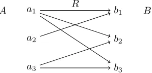
Generalized quantifier theory applied to natural language treats determiners as relations between the denotations of other constituents of a sentence. For example, every is the the inclusion relation: Every student wrote a thesis is true just in case every individual in the set of students is also in the set of thesis-writers. Counting quantifiers such asat least 3 put a restriction on the cardinality of the intersection of two sets: At least 3 students received a mark of 10 on their thesesis true just in case the size of the intersection of the set of students and the set of people receiving a 10 is at least three. For example, we can write the meanings of the quantifiers in these examples as:

every = {(M, A, B) ∶A⊆B}

at least three = {(M, A, B) ∶ ∣A∩B∣≥3}

These are simple examples, but a quantifier may denote a relation between any number of relations of any arity. Mostowski [37] first introduced the general notion of a unary quantifier, binding a single variable in a formula similarly to

∀and∃ in standard logic. Lindstr¨om extended this to arbitrary types.

Definition 2.1.1. [32] A Lindstr¨om quantifierQof type⟨n1, . . . , nk⟩is a class

of modelsM = (M, R1, . . . , Rk)with theRi ni-ary that is closed under

(14)

This definition is the standard in logical settings, while the following appears more often in formal semantics.

Definition 2.1.2. A generalized quantifier assigns ak-ary relationQM to every

set M such that if (R1, . . . , Rk) ∈QM then Ri is ni−ary and is closed under

bijections.

However, they are equivalent due to the following:

(M, R1, . . . , Rk) ∈Q⇔QM(R1, . . . , Rk)

We leave out the subscript and just writeQ(R1, . . . , Rk)orQR1, . . . Rkomitting

parentheses.

If all theniare 1, we sayQis monadic; otherwise it is polyadic. Typical natural

language determiners are type⟨1,1⟩relativizations of type⟨1⟩quantifiers.

Definition 2.1.3. IfQis of type⟨n1, . . . , nk⟩, thenQrelhas type⟨1, n1, . . . , nk⟩

and is defined forA⊆M andRi⊆Mni as:

(Qrel)M(A, R1, . . . , Rk) ⇔QA(R∩An1, . . . , R∩Ank)

Again, we often omit the subscript. For instance, every is the relativization of the familiar ∀ from predicate logic. ∀(B) says that all individuals in the universe are in B. But ∀rel =every restricts the domain of ∀to a new unary relation (set of individuals) contained inM, allowing us to writeevery A B to mean that the elements ofAare also elements ofB. In general we have:

(Qrel₎

M(A, B) ⇔QA(A∩B)

Natural language determiners are generally taken to satisfy certain semantic universals ([3]):

• Qof type⟨1,1⟩satisfies extensionality (EXT) if and only if for allA, B⊆M

andM ⊆M′_:

QM(A, B) ⇔QM′(A, B)

• Qof type⟨1,1⟩is conservative (CONS) if and only if for allM andA, B⊆ M:

QM(A, B) ⇔QM(A, A∩B)

• Q of type ⟨1,1⟩satisfies isomorphism closure (ISOM)1 if and only if for allA, B⊆M andA′_{, B}′⊆_M′_{, if}(_{M, A, B}) ≅ (_M′_{, A}′_{, B}′)_:

QM(A, B) ⇔QM′(A′, B′)

EXT says that the domain can shrink or expand without affectingQ’s value so long as A and B are untouched. CONS says that only the part ofB that is also in A (A∩B) is relevant to Q’s value (sinceQ restricts the domain to its first argument). ISOM states a sort of topic-neutrality: the identities of the

1_{Note that isomorphism closure is part of our definition of generalized quantifier from the}

(15)

individuals are irrelevant, from which it follows that it is the cardinalities of the sets, and not their particular members, which determineQ’s value.

Theorem 2.1.4. [41] A type ⟨1,1⟩quantifier satisfies CONS and EXT if and only if it is a relativization of a type⟨1⟩quantifier.

Natural language determiners are almost invariably type⟨1,1⟩relativizations. From a given type⟨1,1⟩determiner, we can also recover a type ⟨1⟩ quantifier, representing a noun phrase, byfreezing the first argument2_:

(QA₎

M(B) ⇔QM∪A(A, B)

For instance, we may write Every A is B as the type ⟨1,1⟩ determiner every

applied to(A, B)or equivalently as the type⟨1⟩noun phraseeveryA _{applied to} (B), true if the set of every element ofA(i.e.,A itself) is contained inB. Quantifiers additionally satisfying ISOM (called CE quantifiers) have an equiv-alent representation as binary relations on numbers:

Definition 2.1.5. ForQa type⟨1,1⟩CE quantifier, defineQc _by:

Qc(x, y) ⇔ ∃M andA, B⊆M s.t. ∣A−B∣=x,∣A∩B∣=yandQM(A, B)

Theorem 2.1.6. LetQof type⟨1,1⟩be a CE-quantifier. Then for all M and

A, B⊆M:

Q(A, B) ⇔Qc_(∣_A₋_B_∣_,_∣_A_∩_B_∣)

Throughout this thesis, we will consider only quantifiers having these three semantic properties, which are indeed nearly universal for natural language de-terminers.3

Our earlier example determiners are given by the following binary relations:

everyc₍_{x, y}₎ _⇔ _x₌₀

at least threec₍_{x, y}_{) ⇔} _y_≥₃

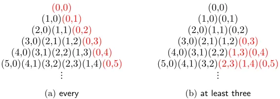
Due to this equivalence with relations on natural numbers, CE quantifiers have a nice geometric representation in the Tree of Numbers ([4]). We can identify

Qwith the pattern in the Tree determined by which pairs(x, y)are inQc_{. The}

Tree also provides an easy characterization of many invariance properties of simple quantifiers, a few of which we mention now.

We say Q is monotone increasing (decreasing) in its right argument, written MON↑ (MON↓) if and only if for all M, A, and B ⊆B′ ₍_B′ ⊆_B_), _Q

M(A, B)

impliesQM(A, B′). Left monotonicity, called persistence (anti-persistence and

written↑MON (↓MON), is defined similarly with respect to taking subsets and

2_{The use of}_M_∪_A_{makes this a global rather than local definition, but the difference does}

not matter here (we will always haveA⊆M).

3_{This assumption puts aside, for example, proper names and, more controversially,}_only.

(16)

(0,0)

(1,0)(0,1)

(2,0)(1,1)(0,2)

(3,0)(2,1)(1,2)(0,3)

(4,0)(3,1)(2,2)(1,3)(0,4)

(5,0)(4,1)(3,2)(2,3)(1,4)(0,5) ⋮

(a)every

(0,0) (1,0)(0,1) (2,0)(1,1)(0,2) (3,0)(2,1)(1,2)(0,3)

(4,0)(3,1)(2,2)(1,3)(0,4)

(5,0)(4,1)(3,2)(2,3)(1,4)(0,5) ⋮

[image:16.612.166.449.125.225.2]

(b)at least three

Figure 2.1: Interpreting quantifiers on the Tree of Numbers

supersets ofA.4 _{We say}_Q_{is (right}₎_continuous_{if for all}_M_,_A_{, and}_B′⊆_B⊆_B′′_,

QM(A, B′)andQM(A, B′′)implyQM(A, B).

Every CE quantifier is the relativizationQrel of a type⟨1⟩quantifierQ. Right montonicity behavior carries over from the monotonicity ofQ. Persistence, or monotonicity in the restricted (left) argument, ofQreldoes not have such a clear relation withQuntil we consider its interpretation in the Tree of Numbers.

b

[image:16.612.207.406.358.417.2]

b

Figure 2.2: Right monotonicity and persistence

b

[image:16.612.207.408.457.517.2]

b b

Figure 2.3: Left and right continuity

Figures 2.2 and 2.3 illustrate what we can infer about the Tree pattern of a quantifier possessing these properties. IfQis monotonic increasing in the right argument, then if a pair (x, y) is in Qc_{, we know that every pair} ₍_{x, y}′)_with y′> _y _{is also in}_Qc_{. If} _Q _{is persistent and} (_{x, y}) _{is in}_Qc_{, then every pair in}

the downward triangle spanned by(x, y)is also inQc (for anti-persistence, it is the upward triangle). Moving down a level in the Tree corresponds to adding an individual to the domain; the downward triangle pattern it does not matter

4_{Often “monotone increasing (decreasing)” is assumed to refer to the right argument, and}

(17)

whether the individual is added toA−BorA∩B. For right continuity, if(x, y)

and (x, y′)_{, with} _y′> _y_{, are in} _Qc_{, then so is every pair in between. For left}

continuity, every pair in the rectangle determined by any two points in Qc is also inQc.

2.1.2 Polyadic Lifts

Monadic quantifiers are sufficient to analyze simple sentences following the schema Q1 A are B, as in Every Olympian is an athlete. However, natural

language is full of examples of polyadic quantification:

(1) Half the students passed every class.

(2) Three researchers published five papers in total. (3) Not all twins are friends.

(4) Five hockey players punched each other.

(5) Some relative of each townsmen and some relative of each villager hate each other.

We restrict the following definitions to the case that apolyadic lift is applied to at most two simple monadic quantifiers, but they may all be defined for an arbitrary number of quantifiers.

Sentence (1) is an example ofiteration. Taking S as the set of students, C as the set of classes, andP= {(s, c) ∶spassedc}, we can give the truth conditions of sentence (1) as:

(half⋅every)(S, C, P) ⇔half(S,{s∶every(C, Ps)})

wherePsis the set{c∶ (s, c) ∈P}. The iteration ofhalf andevery yields a new

quantifierhalf⋅every which takes two sets and a binary relation between them as arguments.

Definition 2.1.7. Let Q1 and Q2 both be of type ⟨1,1⟩. Q1⋅Q2 is the type

⟨1,1,2⟩quantifier such that for allA, B⊆M andR⊆M2_:

(Q1⋅Q2)(A, B, R) ⇔Q1(A,{a∶Q2(B, Ra)})

The iteration of three type⟨1,1⟩quantifiers creates a type⟨1,1,1,3⟩quantifier, and so forth.5

Iterations inherit some nice properties from their components. Zuber [60] ob-serves the following facts (where the relevant notions of monotonicity and con-tinuity of Q1⋅Q2 are obtained by adding or subtracting pairs in the relation

argument):

5_{We can equivalently treat the iteration of two quantifiers as a type}_⟨₂_⟩ _{quantifier by}

freezing the first two arguments:(QA

(18)

• Q1⋅Q2is monotone increasing if and only ifQ1andQ2are both increasing

or both decreasing

• Q1⋅Q2is monotone decreasing if and only if one ofQ1orQ2 is increasing

and the other decreasing

• Q1⋅Q2 is not monotonic if and only if one ofQ1 orQ2 is not monotonic

• IfQ1⋅Q2 is continuous, thenQ1andQ2 are continuous (if non-trivial)6

Sentence (2) is an example of cumulation, meaning that there are three re-searchers such thatall together, they published five papers. Each researcher in the group worked on at least one paper, and each of the five papers was worked on by at least one of the researchers. Compare this to the iterative reading of this sentence, under which we expect each researcher published five papers separately, requiring fifteen total papers.

We denote the cumulation ofQ1 andQ2 by(Q1⋅Q2)cland observe that it can

be defined in terms of iteration:

(Q1⋅Q2)cl(A, B, R) ⇔ (Q1⋅some)(A, B, R) ∧ (Q2⋅some)(B, A, R−1)

This says there is aQ1-sized subset ofA that participates inRand aQ2-sized

subset ofB that participates inR−1_.

Note that we obtain precisely the same truth conditions for a cumulative reading whether the sentence isThree researchers published five papers or Five papers were published by three researchers. This means cumulation is an independent lift. Letlift be any operation taking two type⟨1,1⟩quantifiers and producing a type⟨1,1,2⟩quantifier. Thenliftis independent, corresponding to the order-indifference ofQ1 andQ2, if:

For allM andA, B⊆M, R⊆M2_,_lift₍_Q

1,Q2)M ⇔lift(Q2,Q1)M(B, A, R−1)

Iteration, on the other hand, is generally not order-indifferent. CompareEvery dog chased some cat and Some cat was chased by every dog. In the former, every takes wide-scope, and the sentence may be true when every dog chases a different cat.

Sentence (3) illustrates resumption. Resumption has the effect of lifting Q to quantify over tuples instead of individuals. We define the resumption ofQ, with universeM andR1, R2⊆M2 by:

Resk₍_Q₎

M(R1, R2) ⇔QkM(R1, R2)

We can read the determiner in (3) asRes2₍_{not all}_{) ranging over pairs. Taking}

twins and friends to denote subsets of M2 _{(sets of pairs), we have} _Res2₍_not

all)(twins,friends)if and only iftwins−friends≠ ∅.

Sentence (4) exemplifies reciprocal quantification. Reciprocal quantifiers say there is a large-enough subset of a set whose members participate in a relation

(19)

with one another. Reciprocal quantifiers have many possible interpretations varying in strength depending on the restrictions put on the relation. We can think of the domain A with relation R as the nodes and edge relation of a directed graph. Meanings depend on the following possible interpretations of

R:

• FUL: Every pair inAparticipates inRdirectly (the graph is complete).

• LIN: Every pair inAparticipates inRdirectly or indirectly (the graph is connected).

• TOT: Every element inAparticipates inR directly with some element of

A(every node has an outgoing edge).

[image:19.612.165.443.276.365.2]

(a) TOT (weak) (b) LIN (intermediate) (c) FUL (strong)

Figure 2.4: Models for different interpretations of reciprocals

These interpretations correspond to the following truth conditions7 for the strong, intermediate, and weak readings, depending on whether the relation is FUL, LIN, or TOT, respectively (where∣A∣ is at least 2 andQ is MON↑) ([11],[50]):

• RamS(Q)(A, R) ⇔ ∃X ⊆A[Q(A, X) ∧ ∀x, y∈X(x≠y⇒R(x, y))]

• RamI(Q)(A, R) ⇔ ∃X ⊆A[Q(A, X) ∧ ∀x, y∈X(x≠y⇒ ∃sequence

z1, . . . , zl∈X∶ (z1=x∧R(z1, z2) ∧ ⋯ ∧R(zl−1, zl) ∧zl=y)] • RamW(Q)[A, R] ⇔ ∃X⊆A[Q(A, X) ∧ ∀x∈X∃y∈X(x≠y∧R(x, y))]

We also have Ram∨

S(Q),Ram

∨

I(Q), and Ram

∨

W(Q) with R(x, y) replaced by

R(x, y) ∨R(y, x)in the above definitions (for these alternative readings, think of an undirected graph). This yields at least six possible interpretations8, with the strong meaning implying the intermediate meaning, and the intermediate implying the weak.

To explain how the meaning of a given reciprocal quantifier is chosen from this set of possibilities, Dalrymple et al. [11] propose the strongest meaning hypothesis (SMH), a pragmatic principle predicting that a sentence has the

7_{“Ram” indicates that reciprocal quantifiers are} _{Ramsey lifts. The Ramseyfication of} _Q

expresses that there is aQ-large subset whose members satisfy some formula.

8_{Dalrymple et al. [11] discuss many more potential readings; we present just these six, as}

(20)

logically strongest possible meaning allowed by the context. For example, the meaning ofMost of the children followed one another is underspecified, except insofar as the strong meaning is ruled out sincefollowis an asymmetric relation. Different contextual information may determine different meanings. InMost of the children followed one another through the door, an alternative intermediate interpretation is called for, but inMost of the children followed one another in a circle, the regular intermediate interpretation is possible and logically stronger, and thus is predicted by SMH. Suppose the sentence wereMost of the children followed one another around the museum in small groups: then it seems only the alternative weak reading is available.

An interesting perspective on the meaning of reciprocals is provided by the descriptive complexity results in [50]. Szymanik shows that the strong readings of reciprocal sentences in which the quantifier is counting or proportional are intractable (the problem of determining their truth in a model is NP-complete, since the Ramseyification ofQcan be used to define the clique problem, which is famously NP-complete). He argues this entails that people will disprefer strong readings in such cases in favor of tractable ones based on theP-cognition thesis.9 The variation in complexity of interpretations for reciprocals corroborates SMH but also predicts people will shift to weaker readings though an intractable strong meaning is consistent with the context. [43] presents empirical evidence for this claim.10

Sentence (5) is Hintikka’s sentence, an example of Branching, or partially-ordered, quantification. The idea is thatsome relative of each townsmen(∀x1∃y1)

and some relative of each villager (∀x2∃y2) are chosen independently, so the

truth conditions cannot be given by any first-order sentence since the quanti-fiers would appear in some linear order, introducing scope dependencies. The hallmarks of branching quantification are noun phrases joined byand and re-lations that are in some sense reciprocal; however, the exact conditions are contentious and it is even controversial whether any natural language sentences really have branching meanings.11 _{In general, we define the branching of two}

type⟨1,1⟩MON↑quantifiers as:

Br2(Q1,Q2)(A, B, R) ⇔

∃X⊆A∃Y ⊆B(Q1(A, X) ∧Q2(B, Y) ∧X×Y) ⊆R

Like cumulation, branching is an independent lift.

9_{See footnote 3, page 6 for a reference.}

10_{The experiments confirm that intractable readings do exist in natural language, but that,}

contrary to the Strong Meaning Hypothesis, people strongly disprefer intractable readings and are more error-prone in those cases.

11_{See for example [19] in which Gierasimczuk and Szymanik challenge Hintikka’s thesis}

(21)

2.2 Formal Languages and Automata Theory

This exposition mostly follows Hopcroft and Ullman’sIntroduction to Automata Theory, Languages, and Computation[23], except for Section 2.2.3 which follows Sipser’sIntroduction to The Theory of Computation [44].

Analphabet Σ consists of a finite set of letters (symbols). A finite sequence of letters is aword or string. We sometimes refer to a portion of a given word as asubword. Σ∗ _{denotes the set of all words over Σ. A}_language L _{is some set of}

strings contained in Σ∗_{. Its}_{complement, written} L_{and sometimes}¬L_{, is given}

by Σ∗− L _{(thus a language and its complement always share an alphabet).}

2.2.1 Regular Languages and Finite Automata

Definition 2.2.1. A deterministic finite automaton (DFA) A is a five-tuple

(Q,Σ, δ, s, F)where:

• Qis a finite set of states

• Σ is an input alphabet

• δis a function from Q ×Σ toQ

• s, an element ofQ, is the start state

• F, a subset ofQ, is a set of final states

A DFA is often graphically represented as a set of nodes (the states of the machine, with the start state indicated by an ingoing arrow with no source, and the final states doubly circled) with labeled, directed edges between them (representing the transition function). An edge from q to p labeled a means thatδ(q, a) =p. We can extendδto be defined for entire strings in the obvious way, settingδ(q, w) =δ(δ(q, a), v)where w=av andais a single symbol of Σ. The language ofAis the set of strings wsuch that arun ofA (a computation beginning ins, readingwand transitioning according toδ) ends in a final state:

L(A) = {w∶δ(s, w) ∈F}

A non-deterministic finite automaton (NFA) has a transition relation rather than function, returning a set of states. The machine may have epsilon () moves that don’t consume any input symbol and more than one move per al-phabet symbol in a single state. This reflects the idea that the NFA can non-deterministically “guess” its next move and keep track of every state it might be in. A string w is accepted in case there exists some run ending in a final state, so the language definition forAan NFA becomes:

L(A) = {w∶δ(s, w) ∩F≠ ∅}

(22)

thesubset construction. For an NFAAwith statesQ, its DFAA′_hasP(Q)_for

its set of states. ThusA′_{may have 2}∣Q∣_{-many states, an exponential increase,}

though many of those states will be equivalent. For every DFA accepting a languageLthere is aminimal DFA acceptingL such that any equivalent DFA has at least as many states.

Definition 2.2.2. Regular expressions are algebraic descriptions of sets of strings. We sayE is a regular expression over alphabet Σ ifE is:

1. a∈Σ,, or∅

2. E1+E2, forE1 andE2 regular expressions

3. E1E2, forE1andE2 regular expressions

4. E∗

1, forE1 a regular expression

As with finite automata, we have thelanguage of a regular expression, denoted

L(E). L(E1+E2)isL(E1) ∪L(E2),L(E1E2)isL(E1)L(E2)(the

concatena-tion)12_{, and}_L₍_E∗

1)isL(E1)∗ (the Kleene star or concatenation closure).

Regular expressions and finite automata are equivalent ways of describing the regular languages.

Theorem 2.2.3. [30] If L = L(A) for some DFA A, then there is a regular expression E such that L = L(E). Finite automata and regular expressions generate exactly the same languages (regular languages).

Now we record some useful closure results for regular languages. By Theorem 2.2.3, demonstrating these results by producing a regular expression or finite automaton for the language are both acceptable, but sometimes one method is simpler. We very briefly sketch how these results can be demonstrated by one or the other approach. In the following results, letL1andL2be regular languages

generated by regular expressionsE1andE2and recognized by DFAA1andA2.

Theorem 2.2.4. [30, 2] Regular languages are closed under the Boolean oper-ations of union, intersection, and complementation.

Proof.

• For union closure, connecting a new start states′_{to the start state}_s

1 of

A1 ands2 ofA2 by-transitions yields an NFA recognizing L1∪ L2

• Intersection closure is shown by theproduct construction. TakingQ1×Q2

as the set of states,F1×F2as the set of accepting states, and transitioning

from⟨q, p⟩to⟨q′_{, p}′⟩_{on symbol}_x_if_δ

1(q, x) =q′andδ2(p, x) =p′ yields a

DFA that recognizesL1∩ L2.

• For complementation closure, reversing the accepting and rejecting states (F1 andQ1−F1) ofA1 yields a DFA recognizingL1.

12_The_{concatenation}_of_L

(23)

It is easy to give a regular expression for the union: E1+E2. For the other two,

it is necessary to first construct the automaton and then extract the regular expression.

Theorem 2.2.5. [30] Regular languages are closed under concatenation.

Proof. Connecting final states of A1 to the start state of A2 by -transitions

yields an NFA recognizingL1L2. The corresponding regular expression isE1E2.

Asubstitution sonLwith alphabet Σ is a mapping of eacha∈Σ to a language

La. Forw=a1⋯an∈ L,s(w)is the language of the concatenations(a1)⋯s(an).

Thens(L)is the union of s(w)for allw∈ L.

Theorem 2.2.6. [2] Regular languages are closed under regular substitution.13

Proof. A proof by regular expression mimics the definition above: for L1

gen-erated byE1 with alphabet Σ and a substitution s mapping each a ∈Σ to a

languageLagenerated byEa, replace eachainE1byEa. This yields a regular

expression generatings(L).

The basic idea of the equivalent automaton construction is to replace everya -transition inA by an -transition to a distinct copy ofAa, and for every final

state ofAa add an-transition to the target of the originala-transition.14

2.2.2 Context-free Languages and Pushdown Automata

Now we ascend the Chomsky hierarchy to context-free languages (CFLs), which are strictly stronger than the class of regular languages (REG⊂CFL). Again we have dual formalisms for generation and recognition mechanisms.

Definition 2.2.7. A pushdown automaton (PDA) M is given by a six-tuple

(Q,Σ,Γ, Z0, δ, s, F)where

• Γ is a stack alphabet

• Z0 is a special symbol indicating the bottom of the stack

• δis now a function from Q ×Σ×Γ toP(Q ×Γ)

PDA extend the notion of NFA with astack(the last-in-first-out data structure). The input toδis not only the current state and input symbol but also the top of the stack, and the output of δ is not only a set of states but a set of pairs containing a state and potentially some manipulation of the stack contents: pushing a new symbol or popping the top symbol. If⟨q, x, X, Y, p⟩ ∈δ, meaning

13_{A substitution is regular if the substituted languages are regular.}

14_{The interested reader can see Algorithm 4.2.7 of [36] for a complete description (indeed,}

(24)

δ(q, x, X)contains (p, Y), we may write (q, xw, Xβ) ⊢ (p, w, Y β), wherew is the remainder of the input word, theinstantaneous description ofM describing its step-by-step computatiosn. We write⊢∗ for the transitive closure of ⊢.

A PDA may accept a string by final state or by empty stack. For the former we write

L(M) = {w∶ (s, w, Z0)

∗

⊢ (q, , α)}

whereq is some state inF andαis any string in Γ∗_{, meaning that starting in} swith empty stack and inputw, after some number of stepsM may end up in

qwithαon the stack and having read all ofw. For the latter we write

N(M) = {w∶ (s, w, Z0)

∗

⊢ (q, , )}

whereqis any state at all. Since PDA allow non-determinism, these two accep-tance conditions are equivalent.

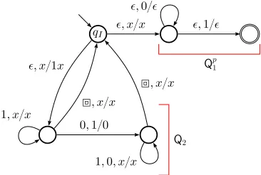
PDA may also be represented graphically with nodes and labeled, directed edges specifying the symbol read and any changes made to the stack. An edge fromq

toplabeledx, X/Y means that inp, if the PDA is readingxand hasX on top of the stack, it may transition top, replacingX byY (i.e. ⟨q, x, X, Y, p⟩ ∈δ).

Definition 2.2.8. A context-free grammar (CFG)Gis given by the four-tuple

(T, V, P, S)where:

• T is a set of terminal symbols

• V is a set of variables

• Pis a set of production rules of the formA→αwithA∈V andα∈ (V∪T)∗ • S is a start symbol

If there are multiple rules whose left-hand side isAwe may combine them into a single rule using “∣” equivalent to “+” for regular expressions, e.g.:

A→α, A→β, . . . ⇒A→α∣β∣ ⋯

We writeÐ→∗ for the transitive closure of→The language of a CFGGis the set of strings of terminals that can be derived from the start symbol:

L(G) = {w∈T∗∶_SÐ→∗ _w}

Theorem 2.2.9. [15] Context-free grammars and pushdown automata are equiv-alent: for every P DA M there is a CFG G such that L(G) = N(P). Thus defining acontext-free language as the language of some CFG is commensurate with defining it as the language of some PDA.

(25)

Proof. The proof idea is the same as with regular languages: given a context-free languageLwith alphabet Σ and a substitutionsmappinga∈Σ to a context-free languageLa: take the CFGGgenerating Land replace eacha (each terminal

in the production rules) with the start symbolSa of Ga generating La. This

yields a CFG generating s(L). The equivalent PDA construction is also very similar to the construction for finite automata.15

Theorem 2.2.11. Context-free languages are closed under concatenation.

Proof. Given G1 generatingL1 andG2 generatingL2, combining them with a

new start symbolS and ruleS→S1S2 yields a CFG generatingL1L2.

CFLs are also closed under union (just combine G1 and G2 with a rule S →

S1∣S2), but are not closed under the remaining boolean operations of

intersec-tion and complementaintersec-tion (thus, sometimes performing these operaintersec-tions with CFLs produces languages in yet stronger classes higher up the hierarchy with context sensitivity, which we do not discuss further here). Suppose CFLs were closed under intersection. LetL1 = {anbncm} and L2 = {ambncn}. These are

both context-free since in each only two numbers must be matched. But their intersection L = {anbncn} is canonically non-context-free. Since closure under complementation and union together yield intersection closure by De Morgan’s laws, we know the former also cannot hold.

2.2.3 Deterministic Context-free Languages and

Deter-ministic Pushdown Automata

Finally we turn to deterministic context-free languages (DCFLs), a proper sub-class of context-free languages. As usual there are production and verification sides to the coin, but they are not entirely equal in this case.

Definition 2.2.12. A deterministic pushdown automaton (DPDA)M is given by a six-tuple(Q,Σ,Γ, Z0, δ, s, F)where:

• δ is a function from Q ×Σ×Γ to(Q ×Γ) ∪ {∅} such that the following condition holds for everyq∈ Q,a∈Σ, andx∈Γ:

exactly one ofδ(q, a, x), δ(q, a, ), δ(q, , x)andδ(q, , )is non-empty.

This ensures that M always has exactly one move per configuration (is deter-ministic).

As with nondeterministic PDA, there are two notions of acceptance defining the language of a DPDA–by final state or by empty stack, which we again denote byL(M)and N(M) respectively–and in this case they diverge. If M accepts

Lby empty stack, we sayLhas theprefix property: ifw∈ L, then there is nov

such thatwv∈ L. In this case, we can constructM′_accepting L_{by final state}

(26)

as follows: M′_simulates_M _on_w_{; if}_M _{reads all of}_w_{and empties its stack,}_M′

transitions to a final state. To convert in the other direction, we forceLto have the prefix property by adding an endmarker to every string, forming L ⊣. If

L =L(M)for someM, then we can constructM′_{such that}L ⊣=_N(_M′)_since M′ _{can recognize the end of the input string and empty its stack if} _M _would

accept the non-endmarked string.

Theorem 2.2.13. [21] DCFLs are closed under complement. For every DPDA

M recognizing a languageL, there is a DPDAM′_recognizing¬L_.

The construction ofM′ _from _M _{is not as easy as complemention for DFA: we}

cannot simply interchange final and rejecting states. Acceptance is defined as entering a final state after reading the input, but a DPDA may enter both final and non-final states after consuming the last input symbol (by making

-moves); in such a case, inverting final and non-final states still results in acceptance. Briefly, the construction requires identifying the set of states that always consume an input symbol (“reading states”). By restricting the final states to this set, the DPDA can only change its accepting behavior if its actually reading input. Interchanging final and rejecting states within the set of reading states produces the complement automaton.

Deterministic context-free grammars are context-free grammars that haveforced handles, which will be made precise shortly.16 DCFGs are still generative de-vices, but to see what makes them deterministic we must take the reverse per-spective and consider their production rules as reduction rules. If u→ v is a step in a derivation expanding a variable in u, then we write v↣uand say v

reducestou. Ifu↣vwhereu=xhyandv=xT y, then this reduction step is the reverse of the substitutionT →h. We callh thehandle of u. A grammar has forced handles if and only if every reducing stepu↣v is uniquely determined by the prefix ofuup to and including its handle.

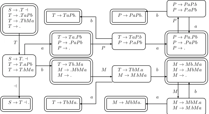
Example 2.2.14. Consider the following deterministic grammar generating the endmarked languagesame number of a’s and b’s17_:

S → T⊣

T → T aP b∣T bM a∣ P → P aP b∣

M → M bM a∣

and the following step in the reduction of a string in the language:

T a P ³¹¹¹¹·¹¹¹¹µ

P aP b b⊣↣T aP b⊣

16_{Sipser defines a DCFG as a LR(0) grammar. A LR(k) grammar may be parsed from left}

to right with alookaheadofk. We will soon see that every DPDA can be minimally modified

such that there is an equivalent DCFG. Since our approach in this thesis in a sense takes automata as primitive, we do not properly introduce the notion of a LR(k) grammar, of which DCFGs are a special case.

17_{The grammar shown is a correction from a list of errata in [44] at}

(27)

This step is the reverse of using the production ruleP →P aP bin the derivation of the string. ThusP is a handle of T aP aP bb, and is indeed forced as there is no other possible handle.

Now we explain theDK-test, a method to decide whether an arbitrary CFG is deterministic.18 The automaton DK for a CFGG= (T, V, P, S)is a DFA that simulates matching the handle of its input. For every ruleB→u1u2. . . uk there

arek+1 dotted rules, one rule per way of placing a dot in the right-hand side (for example, fromA→BCwe obtainA→

.

BC,A→B

.

C andA→BC

.

). To construct theDK DFA, perform the following steps:

1. Put a dot at the initial point in all rules withS on the left-hand side and place these dotted rules inDK’s start state.

2. If there are rules in the state where the dot is immediately followed by a variable C, place dots at the initial points in all rules with C on the left-hand side and add them to the state.

3. Repeat step (2) until no new dotted rules are obtained.

4. For any symbolc(terminal or variable) immediately following a dot, add a c-transition to a state containing dotted rules obtained by shifting the dot to immediately followc in all the rules where the dot was beforec.

5. Repeat steps (2) through (4) for all states until no new states are created.

The final states ofDK are those that contain a completed rule (a rule ended by a dot). Note that there may be cycles inDK, i.e. step (4) does not always create anew state. TheDK-test requires that every final state contains:

• exactly one completed rule,

• no rule where a terminal immediately follows the dot

For example, the DK automaton in Figure 2.5 shows that the grammar in Example 2.2.14 passes the test. Observe that every final state contains exactly one completed rule (having the dot at the end) and no other rule with a terminal symbol (aor b) following a dot.

Theorem 2.2.15. [31] A context-free grammar Gis deterministic if and only if it passes theDK-test.

Theorem 2.2.16. [31] An endmarked language is generated by a DCFG if and only if it is deterministic context-free.

The proof of this theorem consists in showing the following two lemmas. We briefly explain the second for later reference.

Lemma 2.2.17. [31] Every DCFG has an equivalent DPDA.

18_“_DK_{” stands for}_{Donald Knuth, who introduces LR(k) grammars in [31] and describes}

the following test. We present the test for DCFG, but it can be adapted to LR(k) grammars:

“The essential reason behind this [is] thatthe possible configurations of a tree below its handle

(28)

S→.T⊣

T→.T aP b T→.T bM a T→.

S→T.⊣

T→T.aP b T→T.bM a

S→T⊣.

T→T a.P b P→.P aP b P→.

T→T b.M a M→.M bM a M→.

T→T aP.b P→P.aP b

P→P a.P b P→.P aP b P→. P→P aP.b P→P.aP b P→P aP b.

T→T aP b.

T→T bM.a M→M.bM a

M→M b.M a M→.M bM a M→.

M→M bM.a M→M.bM a M→M bM a.

[image:28.612.139.485.127.317.2]

T→T bM a. T ⊣ b a M P a b b a P a M b a b

Figure 2.5: DK example for a grammar generatingL= {w⊣∶#a(w) =#b(w)}

Lemma 2.2.18. [31] Every DPDA recognizing an endmarked language has an equivalent DCFG.

Proof. The DPDA M = (Q,Σ,Γ, Z0, δ, q0, F)is altered to empty its stack and

enter a new accept stateqacceptif it would have accepted originally. This is where

the endmark assumption comes in: M needs an endmarker to recognize the end of the input and implement this behavior. M is also modified to push or pop a (possibly arbitrary) symbol at every step. The DCFG Gwith start symbol

Aqoqaccept is constructed with the following productions:

1-2. For p, q, r∈ Q,u∈Γ anda, b∈Σ∪ {}, ifδ(r, a, ) = (s, u)andδ(t, b, u) = (q, ), addApq→ApraAstb

3 . Forp∈ Q, addApp→

Each variableApqderives all and only the strings on whichM goes frompwith

empty stack toqwith empty stack. Finally,δis extended with the variables of

(29)

Chapter 3

Survey of Semantic

Automata for Monadic

Quantifiers

3.1 Models as Strings

Recall from Section 2.1.1 that if a quantifierQsatisfies CONS, EXT, and ISOM, then it has an equivalent representation as a binary relation on natural numbers

Qc _{such that}

Q(A, B) ⇔Qc_(∣_A₋_B_∣_,_∣_A_∩_B_∣)

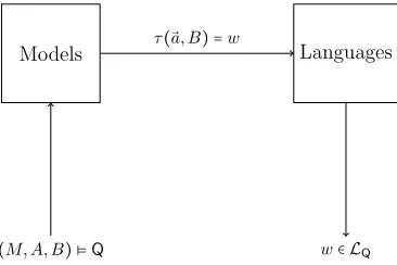
Since the truth ofQ(A, B)depends only on the cardinalities ofAandA∩B, we can record all the information relevant to its evaluation as a string of 0’s and 1’s with one symbol per elementainA: ifais inA∩B, record a 1, otherwise record 0 (ais inA−B). Formally, we can define the following translation function.

Definition 3.1.1. LetM = ⟨M, A, B⟩be a model,a⃗an enumeration ofA, and

n=∣A∣. We defineτ(⃗a, B) ∈ {0,1}n _by

(τ(⃗a, B))i=⎧⎪⎪⎨⎪⎪ ⎩

0 ai∈A−B

1 ai∈A∩B

For example, applyingτ to the model depcited in Figure 3.1, we take any enu-merate⃗aofA, record a 1 or 0 according to which case applies, and concatenate the individual digits. Taking the natural enumeration(a1, a2, a3, a4, a5)yields

the string 00011, but any permutation of this string encodes the same informa-tion, namely that 2a′_s_are_B_{, and 3 are not. Note that}_b

1andb2are irrelevant,

(30)

encodes all the information relevant to the CE quantifiers we are here interested in.

a1

a2

a3

a4

a5

b1

b2

[image:30.612.217.400.484.606.2]

A B

Figure 3.1: Example model to illustrateτ

For a string s∈ {0,1}∗ _{generated by} _τ(⃗_{a, B})_{, let #}

0(s)denote the number of

0’s insand #1(s)the number of 1’s. Then we have

(#0(s),#1(s)) ∈Qc) ⇔ (∣A−B∣,∣A∩B∣) ∈Qc⇔Q(A, B)

Since we have a correspondence between models and strings, we can take the set of strings corresponding to the set of models whereQ is true to constitute thelanguage ofQ:

LQ= {s∈ {0,1}∗∣ (#0(s),#1(s)) ∈Qc}

For example:

Levery = {s∈ {0,1}∗∶#0(s) =0}

Lat least three = {s∈ {0,1}∗∶#1(s) ≥3}

Lsome = {s∈ {0,1}∗∶#1(s) >1}

It is clear by inspecting our example string s = 00011 that s /∈ Levery, s /∈

Lat least three, buts∈ Lsome.

(M, A, B) ⊧Q

Models Languages

w∈ LQ

τ(⃗a, B) =w

(31)

3.2 Semantic Finite Automata

Note that all the results in this section concern quantifiers of type⟨1,1⟩ (equiv-alently, type⟨1⟩), so we often omit the explicit type information.

We will see how semantic finite automataalmost correspond to first-order (FO) definable quantifiers. Definability in FO logic is captured by Ehrenfeucht-Fra¨ıss´e (EF) games.1 _{A formula is FO definable on a finite model if there is an} _n

such that no two models that are indistinguishable up to n disagree on the truth of the formula (and this may be demonstrated by players taking turns choosing elements from the respective models). To begin, we formalize this idea of indistinguishability, which means there is a partial isomorphism between the two models. First, for two sets:

X∼nY if either∣X∣=∣Y ∣=l<nor∣X∣,∣Y ∣≥n

Then define (M, A, B) ∼n (M′, A′, B′) if the relevant sets are ∼n (e.g. A−B

andA′−_B′_,_A∩_B _and_A′∩_B′_,_{. . .}_{). Now we state the general theorem, applied}

to quantifiers.

Theorem 3.2.1. [4] On finite models,Qis FO definable if and only if for some fixedn:

(M, A, B) ∼n(M′, A′, B′)impliesQ(A, B) ⇔Q(A′, B′)

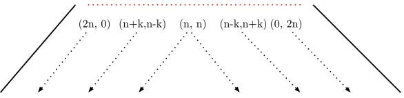
We can interpret this characterization on the Tree of Numbers (recall from Sec-tion 2.1.1), from which it will then be clear that the corresponding languages are regular. For a quantifierQwith its representation in the Tree, after some finite upper triangle the pattern of pairs in the extension is completely predictable. This Fra¨ıss´e threshold occurs at level 2n, and the pattern has the following properties:

• The point(n, n)determines the value of its downward triangle

• The points(n−k, n+k)determine the values of their leftward diagonals

• The points(n+k, n−k)determine the values of their rightward diagonals To see why the Fra¨ıss´e threshold occurs at 2n, note the following:

• In every point(l, m)in the downward triangle generated by(n, n),k, m> n, so the models corresponding to pairs in the triangle are∼n to the model

corresponding to(n, n).

• In every point (l, m) in the leftward diagonal generated by a point(n− k, n+k), k= n and m>n, so the models corresponding to pairs in the diagonal are∼n to the model corresponding to(n−k, n+k). (And clearly

the same holds for(n+k, n−k)to the right).

(32)

(n, n)

(n+k,n-k) (n-k,n+k)

[image:32.612.161.454.124.195.2]

(2n, 0) (0, 2n)

Figure 3.3: Fra¨ıss´e Threshold at level 2n

Theorem 3.2.2. [4] The FO definable quantifiers are precisely those which can be recognized by permutation-invariant acyclic finite state machines.

To see that this holds, it suffices to observe that the Tree patterns corresponding to the languages of the automata are themselves regular. Since the upper trian-gle possibly containing exceptions to the threshold pattern is finite, it is regular. For the pattern below the threshold, note that a triangle under the point(i, j)

is described by at least i 0’s and at least j 1’s, and a leftward diagonal band under (i, j) is described by at least i 0’s and exactly j 1’s (similarly for right diagonal bands). These are all given by regular expressions2 _{(see Appendix A}

for examples).

0

1 0,1

1

[image:32.612.199.406.373.538.2]

0 0,1

Figure 3.4: everyandsome

1 1 1 1

0 0 0 0 0, 1

Figure 3.5: at most three

Acyclic finite automata accept only a proper subset of the regular quantifier languages. DefineDnxϕif and only if the number ofxsatisfyingϕis divisible

by n. These formulae define the “counting modulo” quantifiers: the familiar evenandodd, but alsodivisible by three,divisible by seven, etc. FO(Dω) is

first-order logic extended withDn for alln≥2. Mostowski showed that the class of

2_{Indeed, the Tree itself can be transformed into an automata recognizing the quantifier}

whose pattern it holds. Take the nodes as the points of the upper triangle with 0-transitions from every(i, j)to(i+1, j)and 1-transtions from(i, j)to(i, j+1). For points on the threshold

and to the left of(n, n), let them additionally loop on 0 and go to the right on 1 (opposite

(33)

regular⟨1,1⟩quantifiers are exactly those definable in FO logic augmented with divisiblity quantifiers.

Theorem 3.2.3. [38] Finite automata accept the class of all monadic quantifiers definable in FO(Dω).

1 1

0 0

1

1 1

0

[image:33.612.191.434.196.303.2]

0 0

Figure 3.6: Parity quantifiers: evenanddivisible by 3

We can also use the notion of EF games to demonstrate thatevenis not FO defin-able. This requires showing that for everyn, there are(M, A, B) ∼n(M′, A′, B′)

whereeven(A, B)but¬even(A′_{, B}′)_{. But this is very easy: take two sufficiently}

large models such that∣A∩B∣=m≥nand ∣A′∩_B′∣=_m+_{1. Then they are} ∼n, butevenmust hold in one and not the other.

3.3 Semantic Pushdown Automata

To state results concerning PDA, we need to define a bit of terminology. Say a subset ofNn is a linear set if it is of the form

L(c;{v1, . . . , vr}) = {c+k1v1+ ⋯krvr∶ki∈N,1≤i≤r}

where c, vi ∈ Nn. The vector c is the offset, and the vi are generators. A

semilinear set is a finite union of linear sets. Presburger arithmetic is the FO theory of the natural numbers with addition only (not multiplication). Every Presburger formula defines a set. If a set is Presburger-definable, we equivalently say it is FO additively definable. The FO additively definable sets are exactly the semilinear sets [20].

The Parikh image of a language L with alphabet Σ = {a1, . . . , an}, denoted ψ(L), is the set of vectors:

{(#a1(w), . . . ,#an(w)) ∶w∈ L}

For example, the Parikh image of the languageL1= {0n1n∶n≥0}is the set

con-taining(0,0),(1,1),(2,2), . . ., i.e. the semilinear setψ(L1) =L((0,0);{(1,1)}).

The languageL2 = {w∈ {0,1}∗ ∶#0(w) =#1(w)}has the same Parikh image

(34)

Theorem 3.3.1. [40] For every context-free languageL,ψ(L)is semilinear.

Theorem 3.3.2. [4] Every PDA-computable quantifier is FO additively defin-able.

Given a quantifier Q that is PDA-computable, we know its language LQ is

context-free. Thus the Parikh image of LQ is semilinear, i.e. FO additively

definable. Parikh’s theorem does not convert in general: consider the semilinear setL((0,0,0);{(1,1,1)}), which is the Parikh image of (for example) the non-context-free language {w ∈ {0,1,2}∗ ∶ _#

0(w) = #1(w) = #2(w)}. However,

restricting to a binary alphabet (that is, type ⟨1,1⟩ quantifiers), we have also the following result in the other direction:

Theorem 3.3.3. [4] Every FO additively definable binary quantifier is PDA-computable.

It follows from this theorem that type ⟨1,1⟩ context-free languages are closed under complement, union, and intersection. IfL1 and L2 are such languages,

then they are FO additively definable. Since semilinear sets are closed under these operations, there are formulas defining¬L1,L1∪L2, andL1∩L2, i.e. they

are also context-free.

In [38], Mostowski gives a characterization of quantifiers accepted by DPDA by empty stack; however, he defines somewhat idiosyncratic acceptance conditions that do not align with the standard notion of empty stack acceptance (see Section 2.2.2). He states that the DPDAM accepts a string if the computation ends in a final state, and ifadditionally the stack is emtpy at the end, thatM

accepts the string by empty stack. This has the odd consequence that regular quantifiers are accepted by empty stack, entailing they have the prefix property, which is not in general the case (see Section 2.2.3). Furthermore,no monadic quantifier language has the prefix property (for anywin someLQ, there is always

an extension ofwthat is also inLQ). It appears that the intended notion should

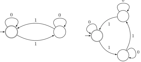
allow the DPDA to transition from a configuration with empty stack (so the language needn’t have the prefix property). Note that in the following results, we refer to this alternative meaning of empty stack acceptance. This meaning does indeed correspond to an interesting subclass of the DPDA-computable quantifiers.

There is an intuitive way to think of these quantifiersQthat are computable by DPDA that happen to have an empty stack when acceptingw∈ LQ, but may

also lead to empty stack configurations at some point mid-computation. The stringswin their languages have the following property:

w=uv∈ LQ andu∈ LQ ⇒v∈ LQ

MoL 2014 14: An Automata Theoretic Perspective on Polyadic Quantification in Natural Language

An Automata-Theoretic Perspective on Polyadic

Quantification in Natural Language

MSc Thesis

(Afstudeerscriptie)

MSc in Logic

Contents

Chapter 1

Introduction

1.1

Motivations and Contributions

1.2

Themes

1.2.1

Meaning as Algorithm

1.2.2

Determinism

1.2.3

Production vs. Recognition

1.2.4

Compositionality

1.2.5

Representation

1.3

Overview

Chapter 2

Prerequisites

2.1

Generalized Quantifier Theory

2.1.1

Properties of Simple Monadic Quantifiers

2.1.2

Polyadic Lifts

2.2

Formal Languages and Automata Theory

2.2.1

Regular Languages and Finite Automata

2.2.2

Context-free Languages and Pushdown Automata

2.2.3

Deterministic Context-free Languages and

Deter-ministic Pushdown Automata

.

.

.

Chapter 3

Survey of Semantic

Automata for Monadic

Quantifiers

3.1

Models as Strings

3.2

Semantic Finite Automata

3.3

Semantic Pushdown Automata