Constructing Semantic Automata for Quantifier Iterations
Sarah McWhirter
Center for Biostatistics in AIDS Research
Harvard T.H. Chan School of Public Health 651 Huntington Avenue, FXB 543
Boston, MA 02115
Jakub Szymanik
Institute for Logic, Language, and Computation University of Amsterdam
Science Park 107 1098 XG Amsterdam
The Netherlands [email protected]
Abstract
We expand on recent work extending the se-mantic automata model of quantifier verifica-tion to iteraverifica-tion. We demonstrate a simple and intuitive method to construct a minimal itera-tion DFA from two DFA recognizing monadic regular quantifier languages and prove that de-terministic CFL are also closed under quanti-fier iteration. We also touch upon the relation between computational results and linguistic discussion of Frege boundary.
1 Introduction
Nearly thirty years ago, van Benthem first intro-duced the notion of semantic automata, uniting gen-eralized quantifier theory (GQT) and formal lan-guage theory in an elegant and powerful way. The basic idea is to use insights of GQT to identify a natural language quantifier with an automaton that, in a precise sense, recognizes the models in which it is true, letting us consider the quantifier as a pro-cedure for checking whether it holds. This marriage enables the use of the Chomsky hierarchy as a mea-sure of complexity of quantifiers, which “turns out to make eminent sense, both in its coarse and fine structure” [2].
Semantic automata have not only led to many ob-servations interesting in their own theoretical right, but also to myriad insights in cognitive modeling and formal learning based on the idea of meaning as algorithm [9, 5, 25, 4]. A steady flow of research was inspired by semantic automata in the following decades, but very little work has been done toward
broadening the model to address more than sim-ple monadic quantifiers, though the definability of polyadic quantification is much-studied. Szymanik [24] provides a computational complexity (Turing machine-based) perspective on polyadic quantifiers, showing that some of those natural language con-structions are polynomial-time closed and others are NP-hard. Those results prompt the question: can we also obtain automata characterizations for some polyadic quantifiers?
2 Prerequisites
2.1 Generalized Quantifiers
In this section we recall a few basic concepts of GQT and refer readers to [20] for more information. GQT applied to natural language treats determiners as re-lations between the denotations of other constituents of a sentence. For example, every is the inclusion relation: Every student wrote a thesisis true just in case every individual in the set of students is also in the set of thesis-writers. We can write the meanings of the quantifiers as:
every = {(M, A, B) ∶A⊆B} at least three = {(M, A, B) ∶ ∣A∩B∣≥3}
These are simple examples, but a quantifier may de-note a relation between any number of relations of any arity. Mostowski [18] first introduced the gen-eral notion of a unary quantifier, binding a single variable in a formula similarly to∀and∃in standard logic. Lindstr¨om extended this to arbitrary types.
Definition 2.1. [16] A Lindstr¨om quantifier Q
of type ⟨n1, . . . , nk⟩ is a class of models M =
(M, R1, . . . , Rk) with the Ri ni-ary that is closed
under isomorphism.
Monadic quantifiers (i.e. of type⟨1, . . . ,1⟩) are suf-ficient to analyze simple sentences following the schemaQ1A are B, as inEvery Olympian is an ath-lete. However, natural language is full of examples of polyadic quantification, such as the following it-eration:
Half the students passed every class.
Taking S as the set of students, C as the set of classes, andP = {(s, c) ∶spassedc}, we can give the truth conditions of this sentence as:
(half⋅every)(S, C, P)
⇔half(S,{s∶every(C, Ps)})
wherePs is the set{c ∶ (s, c) ∈ P}. The iteration
ofhalfandeveryyields a new quantifierhalf⋅every
which takes two sets and a binary relation between them as arguments.
Definition 2.2. LetQ1andQ2both be of type⟨1,1⟩.
Q1⋅Q2is the type⟨1,1,2⟩quantifier such that for all
A, B⊆M andR⊆M2:
(Q1⋅Q2)(A, B, R) ⇔Q1(A,{a∶Q2(B, Ra)})
The iteration of three type⟨1,1⟩quantifiers creates a type⟨1,1,1,3⟩quantifier, and so forth.
Natural language determiners are generally taken to satisfy certain semantic universals [1] yielding so-called CE-quantifiers:
• Qof type⟨1,1⟩satisfies extensionality (EXT) if and only if for allA, B⊆MandM ⊆M′:
QM(A, B) ⇔QM′(A, B)
• Qof type⟨1,1⟩is conservative (CONS) if and only if for allM andA, B⊆M:
QM(A, B) ⇔QM(A, A∩B)
• Qof type ⟨1,1⟩satisfies isomorphism closure (ISOM)1 if and only if for all A, B ⊆ M and
A′, B′⊆M′, if(M, A, B) ≅ (M′, A′, B′):
QM(A, B) ⇔QM′(A′, B′)
Definition 2.3. For Q a type ⟨1,1⟩ CE quantifier, defineQcby:
Qc(x, y) ⇔ ∃M andA, B⊆M s.t.
∣A−B∣=x,∣A∩B ∣=yandQM(A, B)
Theorem 2.4([2]). Let Q of type⟨1,1⟩ be a CE-quantifier. Then for allM andA, B⊆M:
Q(A, B) ⇔Qc(∣A−B∣,∣A∩B ∣)
2.2 Regular and Deterministic Context-free Languages
We assume familiarity with formal language theory [10], but recall a few definitions and key results for later reference, mostly following [21].
Definition 2.5. A deterministic finite automaton (DFA) A is a five-tuple(Q,Σ, δ, s, F) where Q is a finite set of states, Σ is an input alphabet,δ is a function fromQ ×ΣtoQ, s∈ Q is the start state, andF⊆ Qis a set of final states.
A DFA is often graphically represented as a set of nodes (the states of the machine, with the start
1Note that isomorphism closure is part of our definition of
state indicated by an ingoing arrow with no source, and the final states doubly circled) with labeled, di-rected edges between them (representing the tran-sition function). An edge from q to p labeled a
means thatδ(q, a) = p. We can extendδ to be de-fined for entire strings in the obvious way, setting
δ(q, w) =δ(δ(q, a), v)wherew=avandais a sin-gle symbol ofΣ. The language of A is the set of stringswsuch that arunofA(a computation begin-ning ins, readingwand transitioning according to
δ) ends in a final state:
L(A) = {w∶δ(s, w) ∈F}
The set of languages accepted by some DFA are the regular languages (REG). REG has nice clo-sure properties, including cloclo-sure under concatena-tion, substituconcatena-tion, and complementation. These re-sults are all easily proven via automata construction; however, while the first two generally result in non-deterministicfinite automata due to the addition of
transitions, the complement is obtained by switching final and non-final states.
Deterministic context-free languages(DCFLs) are a proper subclass of context-free languages.
Definition 2.6. A deterministic pushdown au-tomaton (DPDA) M is given by a six-tuple
(Q,Σ,Γ, Z0, δ, s, F)where:
• δ is a function fromQ ×Σ×Γ to (Q ×Γ) ∪ {∅}such that the following condition holds for everyq∈ Q,a∈Σ, andx∈Γ:
exactly one ofδ(q, a, x), δ(q, a, ), δ(q, , x)
andδ(q, , )is non-empty.
This ensures that M always has exactly one move per configuration (is deterministic).
DPDA extend DFA with a stack (the last-in-first-out data structure) having push and pop operations. They may accept by final state or empty stack, but these notions are equivalent for end-marked lan-guages.
Like REG, CFL is closed under concatenation and substitution, but not complementation. DCFL is closed under complementation (see Lemma 5.1), but not substitution.
2.3 Semantic Automata for Monadic Quantifiers
Recall that if a quantifier Q satisfies CONS, EXT, and ISOM, then it has an equivalent representation as a binary relation on natural numbersQcsuch that
Q(A, B) ⇔Qc(∣A−B∣,∣A∩B ∣)
Since the truth ofQ(A, B)depends only on the car-dinalities ofAandA∩B, we can record all the in-formation relevant to its evaluation as a string of 0’s and 1’s with one symbol per element a inA: if a
is inA∩B, record a 1, otherwise record 0 (ais in
A−B). Formally, we can define the following trans-lation function.
Definition 2.7. Let M = ⟨M, A, B⟩ be a model,
⃗
a an enumeration of A, and n =∣ A ∣. We define
τ(⃗a, B) ∈ {0,1}nby
(τ(⃗a, B))i=⎧⎪⎪⎨⎪⎪
⎩
0 ai∈A−B
1 ai∈A∩B
For a string s ∈ {0,1}∗ generated by τ(⃗a, B), let #0(s)denote the number of 0’s insand#1(s)the number of 1’s. Then we have
(#0(s),#1(s)) ∈Qc
⇔ (∣A−B∣,∣A∩B∣) ∈Qc ⇔Q(A, B)
Since we have a correspondence between models and strings, we can take the set of strings corre-sponding to the set of models where Q is true to constitute thelanguageofQ:
LQ = {s∈ {0,1}∗∶ (#0(s),#1(s)) ∈Qc} For example:
Levery = {s∈ {0,1}∗∶#0(s) =0}
Lexactly three = {s∈ {0,1}∗∶#1(s) =3}
Leven = {s∈ {0,1}∗∶#1(s)mod2=0}
Lhalf = {s∈ {0,1}∗∶#1(s) =#0(s)} This opens up the application of automata theory to generalized quantification.
Theorem 2.9. [19] Finite automata accept the class of all monadic quantifiers definable in FO logic ex-tended with all divisibility quantifiers.
For example,exactly threeandevery, which are FO definable, are accepted by the respective automata in Figure 2. To account for the “counting modulo” quantifiers such as every, which are not FO defin-able, we need automata with loops. We will refer to quantifiers with languages accepted by finite au-tomata asregular quantifiers.
Theorem 2.10. [2] Every PDA-computable quanti-fier is FO additively definable.
Theorem 2.11. [2] Every FO additively definable binary quantifier is PDA-computable.
This means that the proportional quantifiers such as
halforat least two-thirdsneed the extra computing power of a stack to keep track of the relative number of 1’s and 0’s. Similarly, we refer to such quantifiers as(deterministic) context free quantifiers.
3 New Proof of Closure under Iteration
Shane Steinert-Threlkeld and Thomas Icard III made the first foray into semantic automata for polyadic quantifiers with their paper [23]. First we present a convention for translating models with bi-nary relations into strings. Then we reprove the results that regular and context-free languages are closed under quantifier iteration in a cleaner fash-ion that makes explicit the intuitfash-ions grounding their proofs.
In order to talk about the language accepted by an automaton for an iterated quantifier, we need a way of translating models withnon-unary relationsinto strings.2 The idea is simple: given a binary relation
Rwith domainAand rangeB, look in turn at every elementaofAand record, for each elementbofB, whether or notais in the relationRwithb. To keep the substrings generated by eachadistinguishable, we introduce a new separator symbol⧈.
Example 3.1. A quick example will make the def-inition to follow more intuitive. Figure 1 depicts a
2For simplicity, in this paper, we assume the relations are
binary, but all the results may be easily generalized [17].
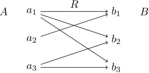
model with setsAandB and a relationRbetween the two. This could represent, for example, a set of aunts, a set of books, and the information regard-ing which aunts read which books. To translate this model into a string, we look at the elements ofAin some order (the indices yield a natural enumeration) and examine which elements ofB they connect to:
a1R’s every element ofB, so we write111⧈;a2R’s only the first element, so we write100⧈;a3R’s the last two elements, so we write011⧈. Concatenating these three substrings yields111⧈100⧈011⧈, which is the string representation of the model.
a1
a2
a3
b1
b2
b3
[image:4.612.352.502.251.325.2]A R B
Figure 1: Example for Definition 3.2
Definition 3.2. LetM = ⟨M, A, B, R⟩be a model,
⃗
aand⃗benumerations ofAandB, and letn=∣A∣. Define a new translation functionτ2which takes two sets and a binary relation as arguments:
τ2(⃗a,⃗b, R) = (τ(⃗b, Rai)⧈)i≤n
whereRai = {b ∈ B ∶ (ai, b) ∈ R}is the set of b
inB in the relationR withai. That is, for eachai,
τ computes a substring with a separator symbol ⧈ appended to the end, recording a 1 ifbjis inRaiand
a 0 otherwise. The final string is the concatenation of all these substrings.
Now languages of iterated type⟨1,1,2⟩ quantifiers are straightforward extensions of languages in the monadic type ⟨1,1⟩ case. Recall that a quantifier
Q1 is equivalently a binary relationQc1 between the number of 1’s and 0’s in the strings of its language. For quantifiers of the formQ1⋅Q2, we let subwords (sequences of 1’s and 0’s separated by ⧈’s) in the language ofQ2replace 1’s and subwords in the com-plement of the language of Q2 replace 0’s as the units upon whichQc1 is defined. Whether or not a subword is in the language ofQ2 is just an instance of the simple monadic case.
def-inition of binary iterations:
(Q1⋅Q2)(A, B, R) ⇔Q1(A,{a∶Q2(B, Ra)})
If we denote the set{a∶Q2(B, Ra)} byX, then a
singlea(yielding a 1 byτ) is inA∩Xif and only ifQ2-manybare inB∩Ra(yielding a string in the
language ofQ2byτ). Thus we also have thatais in
A−X(yielding a 0) if and only if it’s not the case thatQ2-manybare inB∩Ra(yielding a string not
in the language of Q2–equivalently, a string in the complement). Since they are equivalent, we write
w/∈ LQ2andw∈ L¬Q2 interchangeably throughout.
Definition 3.3. LetQ1andQ2be quantifiers of type
⟨1,1⟩. We define the language ofQ1⋅Q2by
LQ1⋅Q2 = {w∈ (wi⧈)∗∶wi∈ {0,1}∗and
(∣ {wi∶wi /∈ LQ2} ∣,∣ {wi∶wi∈ LQ2} ∣) ∈Q1
c}.
Example 3.4. The language of the iterated quanti-fiersome⋅everystill ultimately reduces to a numeri-cal constraint on the number of 1’s and 0’s in strings of the language:
s∈ Lsome⋅every⇔
(∣ {wi∶wi/∈ Levery} ∣,∣ {wi∶wi∈ Levery} ∣)
∈somec⇔∣ {wi∶wi∈ Levery} ∣>0
⇔∣ {wi∶ (#0(wi),#1(wi)) ∈everyc} ∣>0
⇔∣ {wi∶#0(wi) =0} ∣>0
By a similar derivation we get:
s∈ Levery⋅some⇔∣ {wi ∶#1(wi) =0} ∣=0
The string from Example 3.1,111⧈100⧈011⧈, is a member of both these languages, indicating that the sentencesEvery A R some BandSome A R every B are both true in the model depicted by Figure 1.
In the following sections we often speak of words in the language of Q2 without explicitly stating whether we mean words in{0,1}or words ending in
⧈. When considering these strings as input for iter-ation automata, we will make reference to the well-formednessof a string. Call a string well-formedif it ends in⧈. The reader may wonder why we don’t define well-formedness in terms of individual sub-words. To explain this, we must point out that the language accepted by an iteration automaton is in
a sense bigger than the number of relations whose translation it accepts [17]3.
Steinert-Threlkeld and Icard III argue the closure of regular and context-free languages under quantifier iteration via arguments from regular expressions and context-free grammars, respectively. Their intuitive justification does not outright mention the general closure of regular and context-free languages under substitution; however, it is informative to deliber-ately state the fact that quantifier iterationjust isan instance of substitution, from which these closure results follow straightforwardly. In our reformula-tions of their proofs, we define substitureformula-tions directly on languages.
Theorem 3.5. Let LQ1 and LQ2 be languages of
type ⟨1,1⟩ regular quantifiers with alphabetsΣ1 = Σ2= {0,1}. LQ1⋅Q2 is a regular language.
Proof. Define a substitutionsonLQ1 by the
follow-ing:
• s(0) = L¬Q2⧈
• s(1) = LQ2⧈
Claim:s(LQ1) = LQ1⋅Q2
Proof: This is immediately clear from the substitu-tion. Forw = (wi⧈)∗,w ∈ LQ1⋅Q2 if and only if(∣
{wi∶wi ∈ L¬Q2} ∣,∣ {wi∶wi ∈ LQ2} ∣) ∈Q
c
1, if and only ifw=s(w′)where(#0(w′),#1(w′)) ∈Qc1, if
and only ifw∈s(LQ1). ∎
Thussis the appropriate substitution. Since regu-lar languages are closed under complement,L¬Q2 is
regular, and since regular languages are closed under concatenation,L(¬)Q2⧈is regular. Thussdefines a
regular substitution, so by regular substitution clo-sure,s(LQ1) = LQ1⋅Q2 is a regular language.
Theorem 3.6. Let LQ1 and LQ2 be languages of
type ⟨1,1⟩ context-free quantifiers with alphabets Σ1=Σ2= {0,1}.LQ1⋅Q2 is a context-free language.
Proof. We use the same substitutionsonLQ1:
3
For a modelM = (M, A, B, R)withn=∣A∣andm=∣ B∣,τ2generates strings of the form((1+0)m⧈)n, butLQ1⋅Q2
• s(0) = L¬Q2⧈
• s(1) = LQ2⧈
Claim:s(LQ1) = LQ1⋅Q2
Proof: The argument for the previous Claim holds
here as well. ∎
Since context-free quantifier languages are closed under complement4,L¬Q2 is context-free, and since
context-free languages are closed under concate-nation, L(¬)Q2 is context-free. Thus s defines a
context-free substitution, so by context-free substi-tution closure, s(LQ1) = LQ1⋅Q2 is a context-free
language.
4 Constructing minimal iteration DFA
As mentioned previously, the construction in [23] is overly powerful, creating a pushdown automaton as the iteration of two DFA. Their construction of
Q1⋅Q2 consists of a copy ofQ2that pushes a 1 (0) to the stack for every subword in LQ2 (L¬Q2) and
a “pushdown reader”QP1 that “reads” the resulting stack. Further, in that paper they state “There ap-pears to be no such analogously general mechanism for generating minimal DFAs.” Of course, there is great theoretical and practical interest in identify-ing the least-powerful automata recognizidentify-ing iterated quantifiers. The duality between languages and au-tomata makes formal language theory interesting in its own right, and the fact that automata often represent intuitive algorithms for string-membership provides further motivation from the perspective of modeling quantifier verification. We show that, as the iteration closure of regular languages suggests, there is a general method to construct an iteration DFA from two DFA, and furthermore we can di-rectly construct the near-minimal version in every case.
The definition of languages of iterated quantifiers already suggests how to go about constructing it-erated automata from the monadic building blocks. For languages, just replace 1’s in the first by entire
4This follows from Theorem 2.11, since semilinear or FO
definable sets are closed under complement.
words in the language of the second, and 0’s by en-tire words in the complement of the language of the second. To complete the picture, we must ask our-selves,what is the analogous notion in terms of au-tomata? Quite simply, 1-transitionsof the first au-tomaton should be replaced byaccepting runsof the second automaton and0-transitionsreplaced by re-jecting runs.
The main idea is to start withQ1as the backbone of
Q1⋅Q2and then replace each of its states with a copy ofQ2. To make things easier, imagine these copies are indexed by the state they replace. From here on we refer to such copies byQq2and refer to their com-ponents in the obvious way (e.g. Qq2, sq2, δ2q, F2q). If some copyQq2 ends in a final state seeing some sub-word, then the machine should behave as ifQ1 had seen a 1. Suppose q would transition to p on a 1. This means that every final state ofQq2 should tran-sition to the start state ofQp2on⧈(as this marks the end of the subword). Similarly, every rejecting state ofQq2 should have a ⧈-transition to Qr2, wherer is the state thatq would transition to on a 0. Q1⋅Q2 has the same start and final states asQ1.
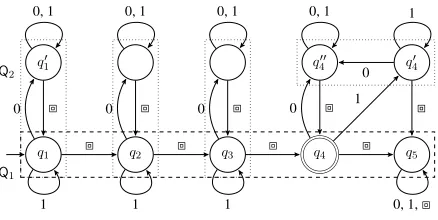
Before giving the formal definition, let us dig a lit-tle deeper with an example. Consider the automa-tonexactly three⋅every depicted in Figure 3. The vestiges of the original state-space ofexactly three
is clearly visible as the “spine” of the automaton, enclosed in the darker dashed box, but the original states have been replaced by copies of every, en-closed in the lighter dashed boxes. There are three exceptions to this simple replacement scheme:
(i) Final states: Notice that the final state of ex-actly three remains externally linked up with a copy of every. This is so that the automa-ton cannot erroneously accept a word ending in 111, for example, which is not well-formed.
(ii) Terminal states: Notice that the terminal state ofexactly threedoesn’t seem to have been re-placed at all. If the automaton reaches stateq5, the rest of the input is irrelevant. The automa-ton canonlyreject at this point, hence the loop-ing on every symbol.
au-tomaton reaches a state that is both final and terminal, it should accept irrespective of the remaining input so long as it is well-formed. Such statesqrequire at most one extra stateeq
to go to in which to loop on 0 and 1 and then return toq on⧈. Ifqhas a predecessor stater
with equivalent behavior, then the extra state is unnecessary (asqmay just go toron 0 and 1).
q 1 q′ 1 1 1
0 0 0 0 0, 1
0
[image:7.612.90.281.195.287.2]0, 1 1
Figure 2:exactly threeandevery
q1 q2 q3 q4 q5
q1′ q′′4 q′4
⧈ ⧈ ⧈ ⧈
⧈ ⧈ ⧈ ⧈ ⧈
0 0 0 0 1
0
0, 1 0, 1 0, 1 0, 1 1
1 1 1 0, 1,⧈
Q2
Q1
Figure 3:exactly three⋅every
As the state-space is given by the replacement scheme, and the 1 and 0-transitions are given by the copies of Q2, all that remains is to specify the ⧈ -transitions, which are determined by the 1 and 0-transitions in the originalQ1. Consider the statesq1 andq′1, together comprisingQq2, replacing q in ex-actly three. Sinceq1is an accepting state inevery, a subrun ending there is analogous to a 1. Thus the⧈ -transition fromq1should mimic the 1-transition ofq toq′, going to the start state of the copy ofQ2 replac-ingq′. Similarly,q′1should mimic the 0-behavior of
q, which is to loop, meaningq′1should return to the start state of theQ2copy of which it is a member.
The final stateq4is not itself a member of any copy ofQ2, but its ⧈ transitions are still decided by the start state of its associated copy ofQ2. If⧈is seen in such a state, this means the current subword was empty; this works because(the empty string) is in
the language ofQ2 if and only if s2 is final, so s2 appropriately determines⧈-behavior.
Definition 4.1. Previously we likened the state space of Q1 to the spine or essential structure of
Q1⋅Q2. Here we make this idea precise by describ-ing a mappdescrib-ing betweenQ1and a subspace ofQ(the state-space of the iteration automaton). Define a bi-jectionf ∶ Q1→ Qby the following:
f(q) =
⎧⎪⎪⎪ ⎪⎪⎪⎪ ⎨⎪⎪⎪ ⎪⎪⎪⎪ ⎩
qF q∈F1, non-terminal
sq2 q/∈F1, non-terminal
qF T q∈F1, terminal
qT q/∈F1, terminal
For example, if a state inQhas the subscriptF, then the corresponding state inQ1 must have been both final and non-terminal. Not every sq2 inQ is f(q)
for someq ∈ Q1, but ifq ∈ Q1is final and non-terminal, it will be merged with the start state of its copy ofQ2. This state mapping will be mostly useful for defining the transition function for the iteration automata. Using this mapping to convert between
q andf(q) and vice versa, we can be sensitive to the above-mentioned exceptions in the replacement scheme while still usingδ1 to defineδ. When the value off for someq is clear, we may write it di-rectly, e.g. “qF T” in lieu of “f(q),” and similarly
for f−1. Sometimes we write, e.g., qT to mean a
specific state, and other times to mean the set of all states that aref(q)for some non-final, terminal state
q. The intention should be clear from the context.
Definition 4.2. Let Q1 = (Q1,Σ1, δ1, s1, F1) and
Q2 = (Q2,Σ2, δ2, s2, F2) be DFAs accepting the monadic quantifier languagesLQ1 andLQ2, respec-tively. The iteration DFAQ1⋅Q2is given by:
• Q: ⋃
q∈Q1
⎧⎪⎪⎪ ⎪⎪⎪⎪ ⎨⎪⎪⎪ ⎪⎪⎪⎪ ⎩
2∪ {qF} q∈F1, non-terminal
2 q /∈F1, non-terminal
{eq, qF T} q∈F1, terminal
{qT} q /∈F1, terminal Here eq is the (potentially unnecessary) state
added to make sure input seen inqF T is
well-formed.
• Σ= {0,1,⧈}
[image:7.612.77.296.328.438.2]– Forp∈ Qq2∶δ(p, x) =
⎧⎪⎪⎪ ⎪⎨ ⎪⎪⎪⎪ ⎩
δq2(p, x) x∈ {0,1}
f(δ1(f−1(p),1)) x= ⧈, p∈F2q
f(δ1(f−1(p),0)) x= ⧈, p/∈F2q
– Forq∈ {qF}:δ(q, x) =δq2(sq2, x)
– Forq∈ {qT}:δ(q, x) =q
– Forq∈ {qF T}:δ(q, x) =⎧⎪⎪⎨⎪⎪
⎩
eq x∈ {0,1}
q x= ⧈
– Forp∈ {eq}:δ(p, x) =⎧⎪⎪⎨⎪⎪
⎩
eq x∈ {0,1}
q x= ⧈
• s=f(s1)
• F = {f(q) ∣q∈F1}
As remarked earlier, the eq may not be necessary,
but whether they are needed is easily seen after δ
has been specified. Once the above construction is completed, one must inspect the state p such that
δ(p,⧈) = q, for eachq inqF T. Ifp also loops on
0 and 1, then eq can be removed, and δ amended
such thatqtransitions topon⧈.
The definition ofQmakes obvious the following up-per bound on the size of iteration DFAs:
Fact 4.3. The state space ofQ1⋅Q2is at most
∑
q∈Q1
⎧⎪⎪⎪ ⎪⎪⎪⎪ ⎨⎪⎪⎪ ⎪⎪⎪⎪ ⎩
∣ Q2∣ +1 q∈F1, non-terminal
∣ Q2∣ q/∈F1, non-terminal 2 q∈F1, terminal
1 q∈F1, non-terminal
This fact gives us the state complexity of iteration DFA, which is a worst-case notion of state-space size5, and thus an upper bound.6 Since our
defini-5See [8] for an overview of the concept. “The
state com-plexityof a regular languageL . . .is the number of states of its minimal DFA,” and “[t]hestate complexity of an operation(or operational state complexity) on regular languages is the worst-case complexity of a language resulting from the operation, con-sidered as a function of the state complexities of the operands.”
6
In [22] (2014), Steinert-Threlkeld also gives a definition (developed independently) of iteration DFA for type⟨1,1,2⟩ regular iterations (different to the PDA construction developed in [23]). His definition uses the cross-product ofQ1andQ2for
the state space with an “unrolled” version ofQ2 with an extra
state ifs2is final. This leads to a state complexity of∣ Q1 ∣ ⋅ ∣
tion uses cases, it is generally tight for any language. Iteration DFA may have fewer states if, as discussed above, extra stateseqare not needed to ensure
well-formedness of the input (see Figure 4). Thus, the size of Q1 ⋅Q2 is generally within m =∣ {qF T} ∣
of this upper bound (and m is at most 1 for reg-ular quantifiers). It is also possible for unforseen state equivalences to occur (see, for example, Figure 5), but such minimizations are similarly restricted to “end behavior.”
q1 q2
1 ⧈
0, 1 0, 1
0,⧈ ⧈
(a)some⋅some
p1 p2
ep2
⧈
0 ⧈ 0, 1 ⧈
0, 1
⧈
1 0, 1
[image:8.612.319.538.220.314.2](b)some⋅every
Figure 4: In (a), the terminal final stateq2of the outer
somecan0,1-transition to the terminal state of the em-beddedsome. In (b), our definition correctly predicts the necessity ofep2.
0 1
1 1 1
⧈
1
⧈ ⧈
⧈ ⧈
⧈
0 0 0 0
1
0, 1
0, 1,⧈
Figure 5: every⋅exactly three. Solid lines indicate the minimal DFA. Dashed lines indicate the output of the construction, with a full copy ofexactly three.
We now make explicit the correctness of the defini-tion of iteradefini-tion automata by showing that the lan-guage accepted by the automaton constructed from the automata for regular quantifiersQ1 andQ2 and the languageLQ1⋅Q2 are equivalent. To prove this,
we first introduce a bit more helpful terminology and a preliminary lemma. Define a function g ∶
{0,1}∗→ {0,1}by:
Q2+1∣. Using the functionfto distinguish different cases in defining the state space, we achieve a smaller state complexity that only reaches∣ Q1 ∣ ⋅ ∣ Q2+1 ∣in caseQ1 is a trivial
[image:8.612.319.541.395.496.2]g(w) =⎧⎪⎪⎨⎪⎪
⎩
0 w/∈ LQ2
1 w∈ LQ2
so g is the characteristic function of LQ2, and let g′(w) = g(wi)i≤#⧈(w), wherew∈ (wi⧈)
∗. For
ex-ample, lettingQ2=every, we can calculateg′(111⧈ 101⧈) =g(111)g(101) =10.
Using gand the function f from Definition 4.1, in the following lemma we prove the intuition ground-ing our construction in the first place: that transitions on words in the language ofQ2and its complement inQ1⋅Q2 are somehow equivalent to transitions on 1’s and 0’s in Q1. See Figure 6 for an illustration of this idea. Given this correspondence, the desired result will be easy to see.
Lemma 4.4. Forwi ∈ {0,1}andp=f(q)for some
q ∈ Q1, δ(p, wi⧈) = f(δ1(f−1(p), g(wi))). This
means that the stateQ1⋅Q2reaches frompreading
wi⧈ is the result of applyingf to the state that Q1 reaches fromf−1(p)readingg(wi).
p f(q)
δ(p, wi⧈)
f−1(p) f−1
q δ1(f−1(p), g(wi))
f
Figure 6: Diagram for Lemma 4.4
Proof. There are four cases to consider, depending on what kind of statepis:
(i) sq2: Suppose wi ∈ LQ2. Then δ(s
q
2, wi) = p
where p ∈ F2q, and δ(p,⧈) = f(δ1(q,1)), which is precisely f(δq(f−1(sq2), g(wi))).
The case forwi /∈ L2is symmetric.
(ii) qF: Suppose wi ≠ , so wi = xwi′ where
x∈ {0,1}. Thenδ(qF, x) ∈ Qq2, and this col-lapses to case (i). Supposewi=, and∈ LQ2,
so g(wi) = 1. Then δ(qF,⧈) = δ(sq2,⧈) =
f(δ1(q,1)), since sq2 ∈ F
q
2 (and similarly if
/∈ LQ2).
(iii) qF T: Since q = f−1(qF T) is terminal,
δ1(q, g(wi)) =q. Ifwi =, thenδ(qF T,⧈) =
qF T =f(q). If not, thenδ(qF T, wi) =eq, and
δ(eq,⧈) =qF T =f(q).
(iv) qT: Again, q = f−1(qT) is terminal, so
δ1(q, g(wi)) =q, andδ(qT, wi⧈) =qT =f(q).
Theorem 4.5. The language accepted byQ1⋅Q2is
LQ1⋅Q2.
Proof. It follows from Lemma 4.4 that if w is a string of the form(wi⧈)∗,Q1⋅Q2acceptswvisiting a sequence of statesss1
2 q1⋯qn (withqi = f(q) for someq ∈ Q1, and possibly repeating) if and only if
Q1accepts the stringg′(w)visiting the sequence of statess1f−1(q1)⋯f−1(qn). That is,w∈ L(Q1⋅Q2) if and only ifg′(w) ∈ LQ1. Butg′(w) ∈ LQ1 if and
only if (#0(g(w)),#1(g(w))) ∈ Qc1, if and only if, by definition, (∣ {wi ∶wi /∈ LQ2} ∣,∣ {wi ∶ wi ∈
LQ2} ∣) ∈Q
c
1, which is the definition of membership forLQ1⋅Q2.
5 Closure of DCFLs under Iteration
Now, it is natural and relevant to ask whether deter-ministiccontext-free quantifier languages, identified recently by Kanazawa [11], are closed under itera-tion. In this section we answer this open question in the affirmative.7 The result is not obvious since DCFLs do not enjoy general substitution closure.
First we establish a sort of normal form for DPDA that is necessary to preserve determinism in the re-sulting iteration automaton.
Lemma 5.1. For every DPDAP recognizing some
LQ that is the language of a deterministic context-free type ⟨1,1⟩ quantifier Q, there is a DPDA P′
with the following properties:
7This closure result was announced independently by Shane
Steinert-Threlkeld and a proof sketch appears in [22], however, it indicates that the DPDA construction proceeds similarly to the DFA case. Since simply complementing the accepting states of a given DPDA may not result in the correct behavior (as it may continue to transition between accepting and rejecting states af-ter reading the input), the correctness of our definitions in this section relies on the modifications described in Lemma 5.1. The cases are not necessarily similar (that is, we can not necessar-ily use a single DPDAQ2to decide ifw∈LQ2 orw∈L¬Q2)
1. P′ has a single accept state qaccept such that
(q0, w⧈, )
∗
⊢ (qaccept, )if and only ifw∈ LQ
2. P′ has a state qreject such that (q0, w⧈, )
∗
⊢ (qreject, )if and only ifw∈ L¬Q
That is, givenP recognizing the language ofQ, we can construct another DPDA that in a sense recog-nizes bothQand¬Qby empty stack given an end-marker.
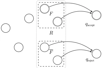
Proof. This follows from the complementation clo-sure of DCFL and the ability to recognize the end of the string. The original DPDA may enter both final and non-final states viamoves after the last symbol, so inverting final and non-final states is in-sufficient to construct the complement. The key is to identify a set of reading statesRwithoutmoves and a new set of final statesF contained inRsuch thatR−F is accepting for the complement of P. Then add a new accept state qaccept and modify the transition function such that the automaton empties its stack and goes toqacceptif it enters a state inF af-ter reading ⧈, satisfying (1). We do the same for a new stateqrejectandR−F, satisfying (2).
F
F
qaccept
[image:10.612.97.277.428.548.2]qreject R
Figure 7:End result of DPDA modification according to Lemma 5.1
Now we can demonstrate the following with a proof by automata8:
Theorem 5.2. Deterministic context-free languages are closed under quantifier iteration.9
8
An alternative proof via iterated grammars and the DK-test (see [15] and [21]) is also presented in [17]
9
Note that, though we state this proof in terms of quanti-fier languages, it applies to the “quantiquanti-fier iteration” of any two binary DPDA-recognizable languages.
Recall that we use the notation ⟨q, x, α, β, q′⟩ for
δ(q, x, α) = (q′, β)for (D)PDA.
Definition 5.3. Let Q1 = (Q1,Σ1,Γ1, δ1, s1, F1) be any DPDA recognizing a deterministic context-free quantifier language LQ1. Let Q2 =
(Q2,Σ2,Γ2, δ2, s2, qaccept, qreject)be a DPDA modified according to Lemma 5.1 recognizing an endmarked deterministic context-free quantifier languageLQ2.
Define the iteration DPDAQ1⋅Q2 by:
• Q = Q1∪ Q2
• Σ=Σ1∪Σ2
• Γ=Γ1∪Γ2∪ Q1
• δ=
δ2 (1)
∪{⟨q, , α, β, q′⟩ ∶ ⟨q, , α, β, q′⟩ ∈δ1} (2)
∪{⟨q, , α, qα, s2⟩ ∶ (q, x, α) ∈dom(δ1) (3) andx∈ {0,1}
∪{⟨qaccept, , qα, β, q′⟩ ∶ ⟨q,1, α, β, q′⟩ ∈δ1} (4)
∪{⟨qreject, , qα, β, q′⟩ ∶ ⟨q,0, α, β, q′⟩ ∈δ1} (5) • s=s1
• F=F1
We take the states ofQ1 and the states ofQ2 and connect them in the following way: for every transi-tion inδ1 in which some stateqreads a symbol, we replace that transition with antransition to the start state of Q2 and push q to the stack. Thus all sub-wordswi⧈of the input are processed byQ2; in any
case,Q2empties its stack up toqand ends up in one ofqaccept orqreject, and transitions back intoQ1—with the new state and new stack contents decided byq.
Of course, natural language iterations often involve a mixture of regular and context-free quantifiers:
(i) A third of the students answered every question correctly.
(ii) Fewer than five students attended more than half of the presentations.
Claim 5.4. The automatonQ1⋅Q2yielded by Defi-nition 5.3 is deterministic.
Proof. First we show this holds when bothQ1 and
Q2 are DPDA. We show there is only one move per configuration inδby examining each part (1)-(5) of the definition:
(1) δ2has at most one move per configuration.
(2) δ1has at most one move per configuration.
(3) A transition of this type is added if q has 0,1 moves inδ1 withαon the stack. This meansq does not have anmove withαon the stack in
δ1 (or a transition with bothinput and stack). Thus, replacing 0,1 withwith α on the stack leavesqwith one choice inδ.
(4) In δ2, qaccept has no moves by construction, and δ1is deterministic, so there is exactly one move inδfor configuration(p, , qα).
(5) The same argument in (4) applies forqreject.
To see the correctness of this definition, we again prove a lemma relating transitions on⧈-ended words inQ1⋅Q2to transitions on individual symbols inQ1.
Lemma 5.5. Letgbe the characteristic function of
LQ2. Forwi ∈ {0,1}∗ andq ∈ Q1,δ(q, wi⧈, α) = δ1(q, g(wi), α).
Proof. LetQ1,Q2 both be DPDA. Assume w.l.o.g. thatqhas 0,1-transitions inδ1(otherwise there is an
-transition to someq′, in both δ1 andδ2, with the same effect on the stack (2)). Then inδ,qhas an -move tos2withqpushed to the stack (3). Sinceqis not inΓ2, this is effectively an empty stack toδ2, so by (1) and Lemma 5.1 we have thatδ(s2, wi⧈, qα)
goes to (qaccept, qα) if g(wi) = 1 or (qreject, qα) if g(wi) = 0. By (4) and (5), there is an -move to
δ1(q, g(wi), α).
Theorem 5.6. The language accepted by the DPDA
Q1⋅Q2isLQ1⋅Q2.
Proof. Given the above lemma, the proof is very similar to that of Theorem 4.5
6 Frege Boundary
Iterations represent a kind of default, the ‘bread and butter’ of multiple quantification in natural lan-guage, hence a popular proposal, so-called Frege’s Thesis: All polyadic quantification in natural lan-guage is iterated monadic quantification.The Frege boundary demarcates the line between reducible and irreducible polyadic quantifiers. Historically, when proposing the boundary, Van Benthem [3] referred to Frege, who introduced the familiar notion of quantification to modern logic. Frege was also the first to give a satisfactory analysis of multiple quan-tification, by simply taking every instance of mul-tiple quantification to be an iteration. Van Benthem calls this ‘solving the problem by ignoring it’—since within this view we can preemptively give an ac-count of any polyadic quantifier in terms of simple monadic quantifiers. Thus, those polyadic quanti-fiers that can be analyzed as iterations of monadic quantifiers are deemedreducible, or simplyFregean. Those that can be given no such analysis are irre-ducibleornon-Fregean, and may be considered gen-uinely polyadic.
(Q1⋅Q2)(A, B, R)is simply Q1aQ2bR(a, b), and thus iteration is monadically definable: this is the sense in which the lift is not taken to be genuinely polyadic. The other lifts, for instance, cumulation and constructions containingsameanddifferentare generally not reducible to iterations. But how we can characterize the Frege boundary? What makes a quantifier non-Fregean?
6.1 Classic Characterization Results
Let us start with a definition to systematize the above discussion:
Definition 6.1. Let us call a type (2) quantifier Fregean if it is an iteration of monadic quantifiers (or a Boolean combination thereof). We say a quan-tifier ‘lies beyond the Frege boundary’ if it is not Fregean.
We proceed historically, starting with the first char-acterization:
combina-tion of iteracombina-tions) if and only if it is both logical and right-oriented.
A quantifier is logical if it is closed under permu-tations of individuals: R ∈ Q if and only if any
π(R) ∈ Q. If S = π(R), we write S ≈ R, and say thatQis closed under≈. A quantifier is right-oriented if it is closed under ∼, where we write
R∼Sif for allx,∣(Rx)∣ = ∣(Sx)∣. This corresponds
to preserving the entire arrow pattern of a relation and preserving the outgoing arrow pattern of a rela-tion.10
[14] provides a characterization that also applies to nonlogical quantifiers and relies on the interesting observation that if two reducible quantifiers behave the same on relations that are cross-products, they actually behave the same on every relation (i.e., are equivalent).
Theorem 6.3([14]). For reducible type(2) quanti-fiersQandQ′,Q=Q′if and only if for all subsets
A, BofM,Q(A×B) =Q′(A×B).
The following equivalent statement of the theorem provides a test for reducibility: if Q(A ×B) =
Q′(A×B) for all A, B ∈ P(M), and we know
Q′ = Q1 ⋅Q2, then Q is reducible if and only if
Q=Q1⋅Q2.
Dekker then generalizes this to quantifiers of arbi-trary arity:
Theorem 6.4([6]). For type(n) quantifiersQand
Q′ that aren-reducible, Q = Q′ if and only if for all subsets A1, . . . , An of M, Q(A1 × ⋯ ×An) =
Q′(A1× ⋯ ×An).
Therefore, Q and Q′ have the same behavior on cross-products and Q′ is reducible, thus Q is re-ducible only if it equalsQ′.
Dekker also defines Q to be invariant for sets in productsifQ(A1× ⋯ ×An) andQ(A′1× ⋯ ×A′n)
imply Q(A1× ⋯ ×A′i× ⋯ ×An) and shows Q is
invariant for sets if and only if it is product equiv-alent to some Q′ = Q1 ○ ⋯ ○Qn.11 Furthermore,
the proof actually constructs the Qi, widening the
10
Van Benthem’s theorem holds forlocal(on a particular fi-nite universe) definability, but can be used to refute definability onanyuniverse [26].
applicability of the Keenan-style reducibility test by removing the problem that ‘maybe one has not tried hard enough’ to find the product-equivalent iteration for comparison.
Example 6.5. Consider the sentenceEvery profes-sor wrote the same number of recommendation let-ters, formalized as (everyP, same numberL)(W). This is product-equivalent to(everyP⋅everyL)(W), since when W is a cross-product relation, every p
is always connected to everyl, and thus incidentally everypis connected to the same number ofl. Since these quantifiers are not the same (take a model in which everyp is connected to the same number of
l, but ∣Wp∣ < ∣L∣), (every,same number) is not
re-ducible toanytwo unary quantifiers.
Other examples of non-Fregean quantifiers include:
• Reflexives (The type (2) quantifier consisting of all reflexive binary relations is not Fregean.), e.g.:
1. Every student is enjoying him/herself.
2. Every company advertises itself.
• Different/different [14], e.g.:
1. Different students answered different questions.
2. Truth-conditions:
∀a≠b∈students∶ answered(a)≠answered(b).
• Dependent comparatives [12], e.g.:
1. A certain number of professors read a much larger number of grad school appli-cations.
2. Truth-conditions:
∣dom(read)∩professors∣ < ∣ran(read)∩applications∣.
• Branching, resumption, cumulatives, Ramseys (see the following chapter for discussion)
11
Dekker nicely sums up what cross-product charac-terizations tell us about iterations:
Not only is this a new and welcome generalization, it also gives some insight into the intimate relation between (n )-reducible type ⟨n⟩ quantifiers and n-ary product relations. If type ⟨n⟩ quantifier
Fnis (n)-reducible. . .thenFnis satisfied byQ1× ⋯ × Qniff each composingfi is
satisfied byQi[6].
Jan van Eijck [7] introduces the notion of (m, n) -reducibility, making it possible to say something about polyadic quantifiers of type(m+n) that are not fully(m+n)-reducible.
Definition 6.6. Q of type (m, n) is (m, n) -reducible if there areQ1 andQ2 of types(m) and
(n)such thatQ=Q1⋅Q2.
Van Eijck also defines the corresponding notions of reducibility equivalence and invariance for sets in products. The striking consequence of generalizing reducibility is the existence of a diamond property and normal form for quantifiers, meaning reducibil-ity is confluent: if a quantifier reduces to two dif-ferent iterations, these reducts must have a common further decomposition. IfQof type(m+n)reduces both toQ1⋅Q2(of types(m)and(n)) and toQ′1⋅Q′2 (of types(m′)and(m+n−m′)), then there exists
Q3(of type(m′−m)) such thatQ=Q1⋅Q3⋅Q′2.
Q
Q1⋅Q2 Q′1⋅Q′2
Q1⋅Q3⋅Q′2
Figure 8: Van Eijck’s diamond property.
Example 6.7. Consider the sentenceEvery teacher assigned different students different problems ana-lyzed as the type⟨3⟩ quantifier (everyT,differentS, differentP) applied to the assignrelation, and let 0
denote the unary quantifier that is false of every set. By Dekker’s results we can see this is not fully 3 -reducible, since it is equivalent to every⋅0⋅0 on
cross-products (i.e., it is true of no cross-product), but obviously is not generally equal toevery⋅0⋅0, since we can construct non-cross-product relations on which itistrue. However, by van Eijck’s results we can also state a positive result, that it is in fact
(1,2)-reducible, equivalent to every⋅(different, dif-ferent). Further, we know it cannot also be(2,1) -reducible to some type(2)Q1 and type(1)Q2, or else by the diamond property there would exist some type(1)Q3making it3-reducible toevery⋅Q3⋅Q2, a contradiction.
6.2 The Frege Boundary and The Chomsky Hierarchy?
The above discussion on the characterization of the Frege boundary was initiated around the time the se-mantic automata were introduced. However, sur-prisingly these two perspectives have not been in much contact and there is still a major unanswered question: Where is the Frege boundary located in the Chomsky hierarchy? One could argue that ir-reducible languages are at least non-context-free as-suming that for the language of a non-Fregean quan-tifier to even make sense the subwords (between⧈) must all have the same length. A simple pump-ing lemma argument demonstrates that no language with an arbitrary number of equal-length subwords is context-free. [17]
Looking at the problem from a somewhat different perspective, we saw a number of characterization re-sults of the Frege boundary. So the question nat-urally arises: is the characterization of the Frege boundaryeffective? That is, given an arbitrary type
(2)quantifier, can one effectively decide whether or not it is an iteration? The computational perspective allows us to ask this question as: given a language
reg-ular quantifiers:
Theorem 6.8([22]). LetL⊆ {0,1,⧈}∗be a regular language. Then it is decidable whether there are reg-ular languagesL1, L2in{0,1}such thatL=L1⋅L2.
The main obstacle to prove the decidability of it-eration for context-free languages is that language equality is undecidable. This leads to the follow-ing conjecture: It is undecidable whether a given context-free languageL in {0,1,⧈} is an iteration of two context-free languages in {0,1}. However, as a corollary of Theorem 3.6 we have:
Corollary 6.9. It is decidable whether a given de-terministic context-free language in {0,1,⧈} is an iteration.
This discussion shows that the interaction between quantifiers and automata raises new and interest-ing questions in both domains (i.e., formal lan-guage theory and generalized quantifier theory). But there’s a lot more to be done if we want to find a genuinely automata-theoretic characteriza-tion of the Frege boundary. Also, irreducible lan-guages will come in different levels of difficulty. How can we further stratify languages of irreducible polyadic quantifiers in terms of the Chomsky hi-erarchy? Right now it seems that to make some progress on these issues one needs find suitable automata/language models and suitable representa-tions (translation funcrepresenta-tions) [17, 22]. In other words, the following questions arise: Are there ways of rep-resenting models that are more appropriate to recog-nizing irreducible quantifiers? How would the lan-guages of specific quantifiers be affected by such ex-tensions, and how would the Frege boundary move up or down the Chomsky hierarchy as a result? And finally, we know hardly anything about the cognitive reality of the Frege boundary.
7 Conclusions
In the paper we have investigated semantic automata for polyadic quantifiers, extending recent results on quantifier iterations. First of all, we have given a new proof that regular and context-free languages are closed under quantifier iterations. Our proof
em-phasizes the explicit link between quantifier itera-tion and the standard concept of substituitera-tion known from formal language theory. Then we have pro-posed an explicit construction for minimal iteration DFA. Furthermore, we have provided a construction for the quantifier iteration of DCFL, hence, solving positively a natural question whether recently identi-fied deterministic context-free quantifiers are closed under iteration.
Natural language also teems with genuinely polyadic quantification [13]. For example, none of the following are definable as or reducible to the iteration of any two monadic quantifiers, and thus are beyond the so-called Frege boundary [3, 14]:
1. Three researchers together published five pa-pers(Cumulation12)
2. Not all twins are friends(Resumption)
3. Six hockey players punched each other (Recip-rocal)
4. Every child read the same book(Same)
5. Most villagers and most townsmen hate each other(Branching)
Given the recent extension to iteration, a next natu-ral pursuit is to account for different forms of irre-ducible quantification with semantic automata. This leads to the question of where the Frege boundary lies in the Chomsky hierarchy. Some challenges to this pursuit are discussed in [17]. For example, the model translation described in this paper is just one possible function that is moreover particularly well-suited for encoding iterations, which are character-ized by closure under right-orientation. Recall the model drawn in Figure 1: all that matters to the truth of an iteration is the number of outgoing ar-rows from each a ∈ A, and not which b ∈ B the arrows point to. For irreducible polyadic quantifi-cation, the identities of the individuals in the model
12
Cumulation is “on the boundary,” definable as a Boolean combination of iterations: (Q1 ⋅ some)(A, B, R) ∧ (Q2 ⋅
somehow contribute to the truth conditions. To iden-tify the same element in different subwords, with the given translation, requires that all subwords have the same length (so we can identify elements by their position). But this alone makes irreducible quan-tifier languages far too complex, and certainly not context-free.
Future work will likely need to explore different model representations to move the project of iden-tifying semantic automata for irreducible quantifiers forward. Additionally, it may be useful to explore automata models that have some sort of back-and-forth functionality, such as two-way automata, mul-tihead and multitape automata, and automata with erasure, as a way of “having a finger on” more than one symbol in the input string at once.
The results in this paper and the possibility of future extensions also lead to many new empirical ques-tions for cognitive modeling and formal learning theory. So far, experimentally measured difficulty in verification has neatly linked up with theoretical complexity, for both fine and more coarse-grained classifications of quantifiers.
We hope these contributions add momentum to the recent revival of interest in semantic automata, spurring further research into automata for polyadic quantifiers, and that the fruits of the algorithmic per-spective on meaning may be brought to bear on prac-tical applications related to multiquantifier construc-tions in natural language.
Acknowledgments
Jakub Szymanik was supported by the The Nether-lands Organisation for Scientific Research Veni Grant NWO-639-021-232.
References
[1] Jon Barwise and Robin Cooper. Generalized quantifiers and natural language. Linguistics and Philosophy, 4(2):159–219, 1981.
[2] Johan van Benthem.Essays in Logical Seman-tics. D. Reidel Publishing Company, 1986.
[3] Johan van Benthem. Polyadic quantifiers. Lin-guistics and Philosophy, 12(4):437–464, 1989.
[4] Robin Clark. On the learnability of quantifiers. In J. van Benthem and A. ter Meulen, editors, Handbook of Logic and Language, chapter 20, pages 911–923. Elsevier,2ndedition, 2011.
[5] Robin Clark and Murray Grossman. Num-ber sense and quantifier interpretation. Topoi, 26(1):51–62, 2007.
[6] Paul Dekker. Meanwhile, within the Frege boundary. Linguistics and Philosophy, 26(5):547–556, 2003.
[7] Jan van Eijck. Normal forms for characteristic functions on n-ary relations. Journal of Logic and Computation, 15(2):85–98, 2005.
[8] Yuan Gao, Nelma Moreira, Rog´erio Reis, and Sheng Yu. A review on state complex-ity of individual operations. Technical re-port, Universidade do Porto, Technical Report Series DCC-2011-08, Version 1.1 (Septem-ber 2012),http://www.dcc.fc.up.pt/ Pubs, 2012.
[9] Nina Gierasimcauk. The problem of learning the semantics of quantifiers. Lecture Notes in Computer Science, 4363:117–126, 2007.
[10] John E. Hopcroft, Rajeev Motwani, and Jef-frey D. Ullman.Introduction to Automata The-ory, Languages, and Computation. Addison-Wesley, 2ndedition, 2001.
[11] Makoto Kanazawa. Monadic quantifiers rec-ognized by deterministic pushdown automata. InProceedings of the 19th Amsterdam Collo-quium, pages 139–146, 2013.
[12] E. Keenan. Further beyond the Frege bound-ary. In J. van der Does and J. van Eijck, edi-tors,Quantifiers, Logic, and Language, CSLI Lecture Notes, pages 179–201. Stanford Uni-versity, California, 1996.
[14] Edward L Keenan. Beyond the Frege bound-ary. Linguistics and Philosophy, 15(2):199– 221, 1992.
[15] Donald E Knuth. On the translation of lan-guages from left to right.Information and Con-trol, 8(6):607–639, 1965.
[16] Per Lindstr¨om. First order predicate logic with generalized quantifiers. Theoria, 32(3):186– 195, 1966.
[17] Sarah McWhirter. An automata-theoretic perspective on polyadic quantification in natural language. Master’s thesis, University of Amsterdam, 2014. http://www.illc. uva.nl/Research/Publications/
Reports/MoL-2014-14.text.pdf.
[18] Andrzej Mostowski. On a generalization of quantifiers. Fundamenta Mathematicae, 44:12–36, 1957.
[19] Marcin Mostowski. Computational semantics for monadic quantifiers. Journal of Applied Non-Classical Logics, 8(1-2):107–121, 1998.
[20] Stanely Peters and Dag Westerst˚ahl. Quanti-fiers in Language and Logic. Clarendon Press, 2006.
[21] Michael Sipser. Introduction to the Theory of Computation. Cengage Learning, 2006.
[22] Shane Steinert-Threlkeld. On the decidability of iterated languages. InProceedings of Phi-losophy, Mathematics, Linguistics: Aspects of Interaction, pages 215–224, 2014.
[23] Shane Steinert-Threlkeld and Thomas F Icard III. Iterating semantic automata. Lin-guistics and Philosophy, 36(2):151–173, 2013.
[24] Jakub Szymanik. Computational complexity of polyadic lifts of generalized quantifiers in natural language. Linguistics and Philosophy, 33(3):215–250, 2010.
[25] Jakub Szymanik and Marcin Zajenkowski. Comprehension of simple quantifiers: Empiri-cal evaluation of a computational model. Cog-nitive Science, 34(3):521–532, 2010.