Interpreting random forest models using a feature contribution method

This is a repository copy of

Interpreting random forest models using a feature contribution

method

.

White Rose Research Online URL for this paper:

http://eprints.whiterose.ac.uk/79159/

Version: Accepted Version

Proceedings Paper:

Palczewska, A, Palczewski, J, Robinson, RM et al. (1 more author) (2013) Interpreting

random forest models using a feature contribution method. In: Information Reuse and

Integration (IRI), 2013 IEEE 14th International Conference on. 2013 IEEE 14th

International Conference on Information Reuse and Integration, 14 - 16 August 2013, San

Francisco, CA, USA. IEEE , 112-119 .

https://doi.org/10.1109/IRI.2013.6642461

[email protected] https://eprints.whiterose.ac.uk/

Reuse

Unless indicated otherwise, fulltext items are protected by copyright with all rights reserved. The copyright exception in section 29 of the Copyright, Designs and Patents Act 1988 allows the making of a single copy solely for the purpose of non-commercial research or private study within the limits of fair dealing. The publisher or other rights-holder may allow further reproduction and re-use of this version - refer to the White Rose Research Online record for this item. Where records identify the publisher as the copyright holder, users can verify any specific terms of use on the publisher’s website.

Takedown

If you consider content in White Rose Research Online to be in breach of UK law, please notify us by

Interpreting random forest models using a feature contribution method

Anna Palczewska

, Jan Palczewski

, Richard Marchese Robinson

, and Daniel Neagu

1,4

Department of Computing, University of Bradford, BD7 1DP Bradford, UK,

School of Mathematics, University of Leeds, LS2 9JT Leeds, UK,

Syngenta Ltd, RG42 6EY Bracknell, UK

[email protected]; [email protected];

richard.marchese [email protected]; [email protected]

Abstract

Model interpretation is one of the key aspects of the model evaluation process. The explanation of the relation-ship between model variables and outputs is easy for sta-tistical models, such as linear regressions, thanks to the availability of model parameters and their statistical signif-icance. For “black box” models, such as random forest, this information is hidden inside the model structure. This work presents an approach for computing feature contributions for random forest classification models. It allows for the de-termination of the influence of each variable on the model prediction for an individual instance. Interpretation of fea-ture contributions for two UCI benchmark datasets shows the potential of the proposed methodology. The robustness of results is demonstrated through an extensive analysis of feature contributions calculated for a large number of gen-erated random forest models.

1. Introduction

Models are used to discover interesting patterns in data or to predict a specific outcome, such as drug toxicity, client shopping purchases, or car insurance premium. They are often used to support human decisions in various business strategies. This is why it is important to ensure model qual-ity and to understand its outcomes. Good practice of model development involves: 1) data analysis 2) feature selection, 3) model building and 4) model evaluation. Implement-ing these steps together with capturImplement-ing information on how the data was harvested, how the model was built and how the model was validated, allows us to trust that the model gives reliable predictions. But, how to interpret an existing model? How to analyse the relation between predicted val-ues and the training dataset? Or which features contribute the most to classify a specific instance? Answers to these

questions are considered particularly valuable in such do-mains as chemoinformatics and predictive toxicology [11]. Linear models, which assign instance-independent coeffi-cients to all features, are the most easily interpreted. How-ever, in the recent literature, there has been considerable focus on interpreting predictions made by non-linear mod-els [4, 8] which do not render themselves to straightforward methods for the determination of variable/feature influence. Of interest to this paper is a popular “black-box model” – the Random Forest model [5]. Its author suggests two mea-sures of the significance of a particular variable [6]: the vari-able importance and the Gini importance. The varivari-able im-portance is derived from the loss of accuracy of model pre-dictions when values of one variable are permuted between instances. Gini importance is calculated from the Gini im-purity criterion used in the growing of trees in the random forest. However, in [9], the authors argue that the above importance measures do not allow for a thorough analysis of a model. Their general representation of variable impor-tance is often insufficient for the complete understanding of the relationship between input variables and the predicted value.

Kuzmin et al. propose in [9] a new technique to calculate the feature contribution, i.e., the contribution of a variable to the prediction, in a random forest model with numerical ob-served values (the obob-served value is a real number). Unlike in the variable importance measures [6], feature contribu-tions are computed separately for each instance/record and provide detailed information about relationships between variables and the predicted value: the extent and the kind of influence (positive/negative) of a given variable. This new approach was positively tested in [9] on a Quantitative Structure-Activity (QSAR) model for chemical compounds. The results were not only informative about the structure of the model but also provided valuable information for the design of new compounds.

contributions applies to random forest models predicting numerical observed values. This paper aims to extend it to random forest models with categorical predictions, i.e., where the observed value determines one from a finite set of classes. The difficulty of achieving this aim lies in the fact that a discrete set of classes does not have the alge-braic structure of real numbers which the approach pre-sented in [9] relies on.

The paper is organised as follows. Section 2 provides a brief description of random forest models. Section 3 presents our approach for calculating feature contributions for binary classifiers, whilst Section 4 describes its exten-sion to multi-class classification problems. Section 5 con-tains applications of the proposed methodology to two real world datasets from the UCI Machine Learning repository. Section 6 concludes the work presented in this paper.

2. Random forest

A random forest (RF) of [5] is a collection of tree pre-dictors grown as follows [6]:

1. the bootstrap phase: select randomly a subset of the learning dataset – a training set for growing the tree. The remaining samples in the learning dataset form a so-called out-of-bag (OOB) set and are used to esti-mate the RF’s goodness-of-fit.

2. the growing phase: grow the tree by splitting the train-ing dataset at each node accordtrain-ing to the value of one from a randomly selected subset of variables (the best split) using classification and regression tree (CART) method [7].

3. each tree is grown to the largest extent possible. There is no pruning.

The bootstrap and the growing phases require an input of random quantities. It is assumed that these quantities are in-dependent between trees and identically distributed. Conse-quently, each tree can be viewed as sampled independently from the ensemble of all tree predictors for a given learning set.

For prediction, an instance is run through each tree in a forest down to a terminal node which assigns it a class. Pre-dictions supplied by the trees undergo a voting process: the forest returns a class with the maximum number of votes. Draws are resolved through a random selection.

To present our feature contribution procedure in the following section, we need a probabilistic interpreta-tion of the forest predicinterpreta-tion process. Denote by C =

{C1, C2, . . . , CK}the set of classes and by∆Kthe set

∆K =

(p1, . . . , pK) :

K X

k=1

pk = 1andpk≥0 .

An element of∆K can be interpreted as a probability

dis-tribution over C. Letek be an element of∆K with1 at

positionk– a probability distribution concentrated at class

Ck. If a treetpredicts that an instanceibelongs to a class

Ckthen we writeYˆi,t =ek. This provides a mapping from

predictions of a tree to the set∆K of probability measures

onC. Let

ˆ

Yi=

1 T

T X

t=1

ˆ

Yi,t,

whereT is the overall number of trees in the forest. Then

ˆ

Yi ∈ ∆K and the prediction of the random forest for the

instanceicoincides with a classCkfor which thek-th

co-ordinate ofYˆiis maximal.1

3. Feature contributions for binary classifiers

The set∆K simplifies considerably when there are two

classes, K = 2. An elementp ∈ ∆K is uniquely

repre-sented by its first coordinate p1 (p2 = 1−p1).

Conse-quently, the set of probability distributions onCis equiva-lent to the probability weight assigned to classC1.

Before we can present our method for computing feature contributions, we have to examine the tree growing process. After selecting a training set, it is positioned in the root node. A splitting variable (feature) and a splitting value are selected and the set of instances is split between the left and the right child of the root node. The procedure is repeated until all instances in a node are in the same class or further splitting does not improve prediction. The class that a tree assigns to a terminal node is determined through majority voting between instances in that node.

We will refer to instances of the training dataset that pass through a given node as the training instances in this node. The fraction of the training instances in a nodenbelonging to classC1 will be denoted byY_meann . It is the probability

that a randomly selected element from the training instances in this node is in the first class. In particular, a terminal node is assigned to classC1ifY_meann >0.5orY_meann = 0.5and

the draw is resolved in favor of classC1.

The feature contribution procedure for a given instance involves two steps: 1) the calculation of local increments of feature contributions for each tree and 2) the aggregation of feature contributions over the forest. For a child node (c) and a parent node (p) the local increment corresponding to a featuref is defined as follows:

LIc

f =   

 

Yc

mean−Ymeanp ,

if the split in the parent is performed over the featuref,

0, otherwise.

1_{The distributionY}ˆ

iis calculated by the functionpredictin the R

A local increment for a featuref represents the change of the probability of being in classC1between the child node

and its parent node provided thatf is the splitting feature in the parent node. It is easy to show that the sum of these changes, over all features, along the path followed by an instance from the root node to the terminal node in a tree is equal to the difference betweenYmean in the terminal and

the root node.

The contributionF Ci,tf of a featuref in a treetfor an

instanceiis equal to the sum ofLIf over all nodes on the

path of instanceifrom the root node to a terminal node. The contribution of a featuref for an instanceiin the forest is then given by

F Cif =

1 T

T X

t=1

F Ci,tf . (1)

The feature contributions vector for an instanceiconsists of contributionsF Cif of all featuresf.

Notice that if the following condition is satisfied:

(U) training instances in each terminal node are of the same class

then

ˆ

Yi=Yr+

X

f

F Cif, (2)

whereYr_{is the coordinate-wise average ofY}

meanover all

root nodes in the forest. If this unanimity condition (U) holds, feature contributions can be used to retrieve predic-tions of the forest. Otherwise, they only allow for the inter-pretation of the model.

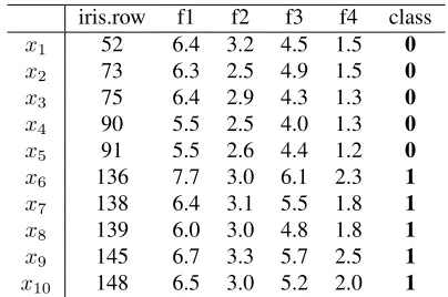
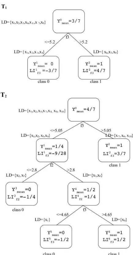
We will demonstrate the calculation of feature contri-butions on a toy example using a subset of the UCI Iris Dataset [3]. From the original dataset, ten records were selected – five for each of two types of the iris plant: ver-sicolor (class 0) and virginica (class 1) (see Table 1). A plant is represented by four attributes: Sepal.Length (f1), Sepal.Width (f2), Petal.Length (f3) and Petal.Width (f4). This dataset was used to generate a random forest model with two trees, see Figure 1. In each tree, the set LD in the root node collects those records which were chosen by the random forest algorithm to build that tree. The LD sets in the child nodes correspond to the split of the above set according to the value of a selected feature (it is written between branches). This process is repeated until reaching terminal nodes of the tree. Notice that the condition (U) for each tree in this forest is satisfied – each terminal node contains instances of the same class:Ymeanis either0or1.

The process of calculating feature contributions runs in 2 steps: the determination of local increments for each node in the forest (a preprocessing step) and the calculation of feature contributions for a particular instance. Figure 1 showsYn

meanand the local incrementLIfcfor a splitting

fea-turef in each node. Having computed these values, we can

iris.row f1 f2 f3 f4 class

x1 52 6.4 3.2 4.5 1.5 0

x2 73 6.3 2.5 4.9 1.5 0

x3 75 6.4 2.9 4.3 1.3 0

x4 90 5.5 2.5 4.0 1.3 0

x5 91 5.5 2.6 4.4 1.2 0

x6 136 7.7 3.0 6.1 2.3 1

x7 138 6.4 3.1 5.5 1.8 1

x8 139 6.0 3.0 4.8 1.8 1

x9 145 6.7 3.3 5.7 2.5 1

x10 148 6.5 3.0 5.2 2.0 1

Table 1: Selected records from the UCI Iris Dataset. Each record corresponds to a plant. Features f1, f2, f3, f4 rep-resent the following attributes: Sepal.Length, Sepal.Width, Petal.Length and Petal.Width. The plants were classified as iris versicolor (class 0) and virginica (class 1).

calculate feature contributions for an instance by running it through both trees and summing local increments of each of the four features. For example, the contribution of a given feature for the instancex1is calculated by summing local

increments for that feature along the pathp1 = n0 → n1

in treeT1and the pathp2=n0→n1 →n4 →n5in tree

T2. According to Formula (1) the contribution of feature f2

is calculated as

F Cf2

x₁ =

1 2

0 + 1

4

= 0.125

and the contribution of feature f3 is

F Cf3

x₁ =

1 2

−3

7 −

9

28−

1 2

=−0.625.

The contributions of features f1 and f4 are equal to 0 be-cause these attributes are not used in any decision made by the forest. The predicted probabilityYˆx1thatx1belongs to class 1 (see Formula (2)) is

ˆ

Yx₁=

1 2

₃

7 +

4 7

| {z } ˆ Yr

+ 0 + 0.125−0.625 + 0

| {z }

P

fF C f x₁

= 0.0

Table 2 collects feature contributions for all 10 records in the example dataset. These results can be interpreted as follows:

• for instancesx1, x3, the contribution of f2 is positive,

i.e., the value of this feature increases the probability of being in class 1 by 0.125. However, the large nega-tive contribution of the feature f3 implies that the value of this feature for instancesx1andx3was decisive in

assigning the class 0 by the forest.

• for instancesx6, x7, x9, the decision is based only on

Figure 1: A random forest model for the dataset from Ta-ble 1. The set LD in the root node contains a local training dataset for the tree. The sets LD in the child nodes corre-spond to the split of the above set according to the value of selected feature. In each node,Yn

meandenotes the fraction

of instances in the LD set in this node belonging to class 1, whilstLIn

f shows non-zero local increments.

• for instances x2, x4, x5, the contribution of both

fea-tures leads the forest decision towards class 0.

• for instancesx8, x10,Yˆ is0.5. This corresponds to

the case where one of the trees points to class 0 and the other to class 1. In practical applications, such sit-uations are resolved through a random selection of the class. SinceYˆr_{= 0.5, the lack of decision of the}

for-est has a clear interpretation in terms of feature

contri-ˆ

Y f1 f2 f3 f4 prediction

x1 0.0 0 0.125 -0.625 0 0

x2 0.0 0 -0.125 -0.375 0 0

x3 0.0 0 0.125 -0.625 0 0

x4 0.0 0 -0.125 -0.375 0 0

x5 0.0 0 -0.125 -0.375 0 0

x6 1.0 0 0 0.5 0 1

x7 1.0 0 0 0.5 0 1

x8 0.5 0 0.125 -0.125 0 ?

x9 1.0 0 0 0.5 0 1

x10 0.5 0 0 0 0 ?

Table 2: Feature contributions for the random forest model from Figure 1.

butions: the amount of evidence in favour of one class is counterbalanced by the evidence pointing towards the other.

4. Feature contributions for general classifiers

When K > 2, the set ∆K cannot be described by a

one-dimensional value as above. We, therefore, generalize the quantities introduced in the previous section to a multi-dimensional case. Yn

meanin a nodenis an element of∆K,

whosek-th coordinate,k= 1,2, . . . , K, is defined as

Ymean,kn =

|{i∈T S(n) : i∈Ck}|

|T S(n)| , (3)

whereT S(n)is the training set in the nodenand| · | de-notes the number of elements of a set. Hence, if an instance is selected randomly from a training set in a node n, the probability that this instance is in classCk is given by the

k-th coordinate of the vectorYn

mean. Local incrementLI c f

is analogously generalized to a multidimensional case:

LIc

f =     

   

Yc

mean−Y p mean,

if the split in the parent is performed over the featuref,

(0, . . . ,0)

| {z } Ktimes

, otherwise,

where the difference is computed coordinate-wise. Simi-larly,F Ci,tf andF C

f

i are extended to vector-valued

quan-tities. Notice that if the condition (U) is satisfied, Equation (2) holds withYr

being a coordinate-wise average of vec-torsYmeanover all root nodes in the forest.

Fix an instance iand let Ck be the class to which the

forest assigns this instance. Our aim is to understand which variables/features drove the forest to make that prediction. We argue that the crucial information is that which explains the value of thek-th coordinate ofYˆi. Hence, we want to

Algorithm 1FC(RF,s)

1: k←f orest predict(RF, s)

2: F C←vector(f eatures)

3: foreach treeT in forestFdo

4: parent←root(T)

5: whileparent! = TERMINALdo

6: f ←SplitF eature(parent)

7: ifS[f]<=SplitV alue(parent)then

8: child←lef tChild(parent)

9: else

10: child←rightChild(parent)

11: end if

12: F C[f]←F C[f] +Y_mean,kchild −Y_mean,kparent

13: parent←child

14: end while

15: end for

16: F C←F C/ nTrees(F)

17: return F C

Algorithm 2Ymean(RF, D)

1: foreach treeT in forestFdo

2: T S←training set for treeT

3: use DFS algorithm to compute training sets in all other nodes n of tree T and compute the vector

Yn

meanaccording to formula (3).

4: end for

Pseudo-code to calculate feature contributions is pre-sented in Algorithm 1. Its inputs consist of a random forest modelRF and an instanceswhich is represented as a vec-tor of feature values. In line 1,k is assigned a prediction of the random forestRF for the instances. The following line creates a vector of real numbers indexed by features and initialized to 0. Then for each tree in the forestRF

the instancesis run down the tree and feature contributions are calculated. The quantitySplitF eature(parent) iden-tifies a featuref on which a split is performed in the node

parent. If the value of that featuref is lower or equal to

the thresholdSplitV alue(parent), the route continues to the left child of the nodeparent. Otherwise, it goes to the right child (each node in the tree has either two children or is a terminal node). A position corresponding to the feature

f in the vectorF C is updated according to the change of values ofYmean,kbetween the parent and the child.

Algorithm 2 provides a sketch of the preprocessing step to computeYn

mean for all nodes n in the forest. The

pa-rameterDdenotes the set of instances used for training of the forestRF. In line 2, T S is assigned the set used for growing tree T. This set is further split in nodes accord-ing to values of splittaccord-ing variables. We propose to use DFS (depth first search) to traverse the tree and compute the

vec-torYn

mean once a training set for a noden is determined.

There is no need to store a training set for a nodenonce

Yn

meanhas been calculated.

5. Applications

In this section, we demonstrate how feature contributions can be applied to improve understanding of a random forest model. An extensive comparative study of feature contri-butions is beyond the capacity of a short conference paper. Therefore, we consider one example of a binary classifier using the UCI Breast Cancer Wisconsin Dataset [1] (BCW Dataset) and one example of a general classifier for the UCI Iris Dataset [3]. We complement our studies with a robust-ness analysis.

5.1. Breast Cancer Wisconsin Dataset

The UCI Breast Cancer Wisconsin Dataset contains characteristics of cell nuclei for 569 breast tissue samples; 357 are diagnosed as benign and 212 as malignant. The characteristics were captured from a digitized image of a fine needle aspirate (FNA) of a breast mass. There are 30 features, three (the mean, the standard error and the aver-age of the three largest values) for each of the following 10 characteristics: radius, texture, perimeter, area, smooth-ness, compactsmooth-ness, concavity, concave points, symmetry and fractal dimension.

To reduce correlation between features, the min-max (minimal-redundancy-maximal-relevance) method was ap-plied and the following features were removed from the dataset: 1, 3, 8, 10, 11, 13, 12, 15, 19, 10, 21, 24, 26. A random forest model was generated on 2/3 randomly se-lected instances using 500 trees. The other 1/3 of instances was used for testing. The test set validation showed that the model accuracy was 0.9682 (only 6 instances out of 189 were classified incorrectly); similar accuracy was achieved when the model was generated using all the features.

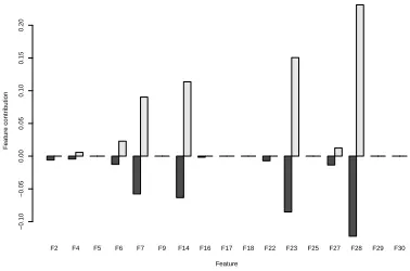
We applied our feature contribution algorithm to the above random forest binary classifier. To align notation with the rest of the paper, we denote the class “malignant” by 1 and the class “benign” by 0. Aggregate results for the fea-ture contributions for all 569 instances and both classes are presented in Figure 2. Light-grey bars show medians2 _of

contributions for instances of class 1 (malignant), whereas black bars show medians of contributions for instances of class 0. Notice that there are only a few significant features in the graph: F7 – the mean of the cell concavity, F14 – the standard deviation of the cell area, F23 – the mean of the cell perimeter and F28 – the average of three largest mea-surements of concave points. This selection of significant

F2 F4 F5 F6 F7 F9 F14 F16 F17 F18 F22 F23 F25 F27 F28 F29 F30 Feature

F

eature contr

ib

ution

−0.10

−0.05

0.00

0.05

0.10

0.15

0.20

Figure 2: Medians of feature contributions for each class for the BCW Dataset. The light grey bars represent contri-butions toward class 1 and the black bars show contricontri-butions towards class 0.

F5 F30 F17 F29 F16 F6 F2 F18 F9 F7 F25 F27 F4 F22 F28 F14 F23

−1 0 1 2 3 4 MeanDecreaseAccuracy

F30 F5 F25 F9 F2 F29 F17 F18 F4 F27 F16 F22 F6 F7 F14 F23 F28

0 5 10 15 20 25 30 35 MeanDecreaseGini

breastrfmtest

Figure 3: The left panel shows permutation based variable importance and the right panel displays Gini importance for a RF binary classification model developed for the BCW Dataset. Graphs generated using randomForest package in R.

features is in agreement with the results of the permutation based variable importance (the left panel of Figure 3) and the Gini importance (the right panel of Figure 3). Interpret-ing the size of bars as the level of importance of a feature, our results are more in line with those provided by the Gini index. However, the main advantage of the approach pre-sented in this paper lies in the fact that one can study the reasons for the forest’s decision for aparticular instance.

Comparison of feature contributions for a particular stance with medians of feature contributions for all in-stances of one class provides valuable information about the forest’s prediction. In a typical case when most of the trees vote for class 1 the feature contributions for that instance are very close to the median values (see Figure 4). This hap-pens in around80%of all instances predicted to be in class 1. However, when the decision is less unanimous, the anal-ysis of feature contributions may reveal interesting infor-mation. As an example, we have chosen instances 194 and

Instance Id benign (class 0) malignant (class 1)

3 0 1

194 0.298 0.702

537 0.234 0.766

Table 3: Percentage of trees that vote for each class in RF model for a selection of instances from the BCW Dataset.

F2 F4 F5 F6 F7 F9 F14 F16 F17 F18 F22 F23 F25 F27 F28 F29 F30 Feature

F

eature contr

ib

ution

0.00

0.05

0.10

0.15

0.20

Figure 4: Comparison of the medians of feature contribu-tions over all instances of class 1 (black bars) with feature contributions for instance number 3 (light-grey bars) from the BCW Dataset.

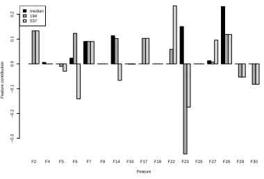
537 (see Table 3) which were classified as malignant (class 1) by a strong majority of trees but with a significant num-ber of trees expressing an opposite view. Figure 5 presents feature contributions for these two instances (grey and light grey bars) against the median values for class 1 (black bars). The largest difference can be seen on the contribution of feature F23: it is highly negative for two instances under consideration compared to a large positive value commonly found in instances of class 1. Recall that a negative value contributes towards the classification in class 0. There are also three new significant attributes (F2, F17 and F22) that contribute towards the correct classification. Feature F22 is judged as moderately important by both of the variable im-portance methods in Figure 3. However, features F2 and F17 are located towards the bottom of both panels. It is, therefore, surprising to note that the contribution of these three new features was instrumental in correctly classifying instances 195 and 537 as malignant. This highlights the fact that features which may not generally be important for the model may, nonetheless, be important for classifying spe-cific instances. The approach presented in this paper is able to identify such features, whilst the standard variable im-portance measures for random forest cannot.

5.2. Iris Dataset

multi-F2 F4 F5 F6 F7 F9 F14 F16 F17 F18 F22 F23 F25 F27 F28 F29 F30 Feature

F

eature contr

ib

ution

−0.3

−0.2

−0.1

0.0

0.1

0.2

median 194 537

Figure 5: Comparison of the medians of feature contribu-tions over all instances of class 1 (black bars) with feature contributions for instances number 194 (grey bars) and 537 (light-grey bars) from the BCW Dataset.

classification models. We generated a random forest model on 100 randomly selected instances. The remaining 50 in-stances were used to assess the accuracy of the model: 47 out of 50 instances were correctly classified. Then we ap-plied our approach for determining the feature contributions for the generated model. Figure 6 presents medians of fea-ture contributions for each of the three classes. In contrast to the binary classification case, feature contributions are positive for all classes. A positive feature contribution for a given class means that the value of this feature directs the forest towards assigning this class. A negative value points towards the other classes.

Feature contributions provide valuable information about the reliability of random forest predictions for a par-ticular instance. It is commonly assumed that the more trees voting for a particular class, the higher the chance that the forest decision is correct. We argue that the analysis of feature contributions offers a more refined picture. As an example, take two instances: 120 and 150. The first one was classified in class Versicolour (88% of trees voted for this class). The second one was assigned class Virginica with 86% of trees voting for this class. We are, therefore, tempted to trust both of these predictions to the same extent. Table 4 collects feature contributions for these instances. Recall that the highest contribution to the decision is com-monly attributed to features 3 (Petal.Length) and 4 (Petal Width), see Figure 6. These features also make the highest contributions to the predicted class for instance 150. The in-decisiveness of the forest may stem from an unusual value for the feature 1 (Sepal.Length) which suggested a different class. In contrast, the instance 120 shows standard (low) contribution of the first two features and unusual contribu-tions of the last two features: very low for feature 3 and high for feature 4. Recalling that features 3 and 4 tend to contribute most to the forest’s decision (see Figure 6) with values between 0.25 and 0.35, the low value for feature

Sepal.Length Sepal.Width Petal.Length Petal.Width Setosa

Versicolour Virginica

Feature

F

eature contr

ib

ution

0.00

0.05

0.10

0.15

0.20

0.25

0.30

0.35

Figure 6: Medians of feature contributions for each class for the UCI Iris Dataset.

Instance Sepal Petal

Length Width Length Width

120 0.059 0.014 0.053 0.448

150 -0.097 0.035 0.259 0.339

Table 4: Feature contributions for selected instances from the UCI Iris Dataset.

3 is non-standard for its predicted class, which increases the chance of it being wrongly classified. Indeed, both in-stances belong to class Virginica while the forest classified the instance 120 wrongly as class Versicolour and the in-stance 150 correctly as class Virginica.

5.3

Robustness analysis

For the validity of the study of feature contributions, it is crucial that the results are not artefacts of one particular realization of a random forest model but that they convey actual information held by the data. We therefore propose a method for robustness analysis of feature contributions. We will use the UCI Breast Cancer Wisconsin Dataset studied in Subsection 5.1 as an example.

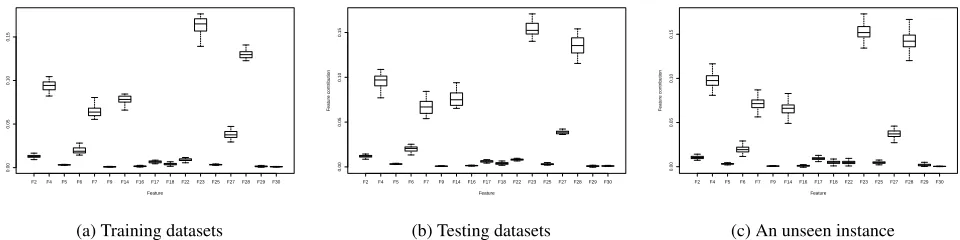
We removed instance number 3 from the original dataset to allow us to perform tests with an unseen instance. We generated 100 random forest models with 500 trees with each model built using an independent randomly generated training set with379≈2/3·568instances. The rest of the dataset for each model was used for its validation. The aver-age model accuracy was 0.963. For each generated model, we collected medians of feature contributions separately for training and testing datasets and each class. The variation of these quantities over models for class 1 and the training dataset are presented using a box plot in Figure 7a. The top of the box is the75%quantile, the bottom is the25%

F2 F4 F5 F6 F7 F9 F14F16 F17F18 F22F23F25 F27F28F29 F30

0.00

0.05

0.10

0.15

Feature

F

eature contr

ib

ution

(a) Training datasets

F2 F4 F5 F6 F7 F9 F14F16 F17F18F22 F23F25F27 F28F29F30

0.00

0.05

0.10

0.15

Feature

F

eature contr

ib

ution

(b) Testing datasets

F2 F4 F5 F6 F7 F9 F14F16F17 F18F22F23 F25F27F28 F29F30

0.00

0.05

0.10

0.15

Feature

F

eature contr

ib

ution

(c) An unseen instance

Figure 7: Feature contributions for 100 random forest models.

5.1 would hold for each of the generated 100 random forest models.

A testing dataset contains those instances that do not take part in the model generation. One can, therefore, expect more errors in the classification of the forest, which, in ef-fect, should imply lower stability of the calculated feature contributions. Indeed, the box plot presented in Figure 7b shows a slight tendency towards increased variability of the feature contributions when compared to Figure 7a. How-ever, these results are qualitatively on par with those ob-tained on the training datasets. We can, therefore, conclude that feature contributions computed for a new (unseen) in-stance provide reliable information. We further tested this hypothesis by computing feature contributions for instance number 3 that did not take part in the generation of models. The statistics for feature contributions for this instance over 100 random forest models are shown in Figure 7c. Similar results were obtained for other instances.

6. Conclusions

Feature contributions provide a novel approach towards black-box model interpretation. They measure the influence of variables/features on the prediction outcome and provide explanations as to why a model makes a particular deci-sion. In this work, we extended the feature contribution method of [9] to random forest classification models and we proposed a framework for the robustness analysis. Using UCI benchmark datasets we showed the robustness of the proposed methodology. We also demonstrated how feature contributions can be applied to understand the dependence between instance characteristics and their predicted classi-fication and to assess the reliability of the prediction. The relation between feature contributions and standard variable importance measures was also investigated. The software used in the empirical analysis was implemented in R as an add-on for the randomForest package and is currently be-ing prepared for submission to CRAN [2]. Application of

feature contributions for model interpretation is particularly valuable for drug discovery or predictive toxicology, which is the topic of our ongoing research.

Acknowledgements. This work is partially supported by BBSRC and Syngenta Ltd through the Industrial CASE Studentship Grant (No. BB/H530854/1).

References

[1] Breast Cancer Wisconsin Diagnostic dataset. http:// archive.ics.uci.edu/ml/datasets/Breast+ Cancer+Wisconsin+\%28Diagnostic\%29. [2] CRAN - The Comprehensive R Archive Network. http:

//cran.r-project.org/.

[3] Iris dataset. http://archive.ics.uci.edu/ml/ datasets/Iris.

[4] D. Baehrens, T. Schroeter, S. Harmeling, M. Kawanabe, K. Hansen, and K.-R. Muller. How to explain individual classification decisions. Journal of Machine Learning Re-search, 11:1803–1831, 2010.

[5] L. Breiman. Random forests. Machine Learning, 45(1):5– 32, 2001.

[6] L. Breiman and A. Cutler. Random forests. http://www.stat.berkeley.edu/˜breiman/ RandomForests/, 2008.

[7] L. Breiman, J. H. Friedman, R. A. Olshen, and C. J. Stone. Classification and regression trees. Monterey, CA: Wadsworth & Brooks/Cole Advanced Books & Software, 1984.

[8] K. Hansen, D. Baehrens, T. Schroeter, M. Rupp, and K.-R. Mller. Visual interpretation of kernel-based prediction models.Molecular Informatics, 30(9):817–826, 2011. [9] V. E. Kuz’min, P. G. Polishchuk, A. G. Artemenko, and S. A.

Andronati. Interpretation of qsar models based on random forest methods. Molecular Informatics, 30(6-7):593–603, 2011.

[10] A. Liaw and M. Wiener. Classification and regression by randomforest.R News, 2(3):18–22, 2002.